Convergence and coupling for spin glasses and hard spheres

Abstract

We discuss convergence and coupling of Markov chains, and present general relations between the transfer matrices describing these two processes. We then analyze a recently developed local-patch algorithm, which computes rigorous upper bound for the coupling time of a Markov chain for non-trivial statistical-mechanics models. Using the “coupling from the past” protocol, this allows one to exactly sample the underlying equilibrium distribution. For spin glasses in two and three spatial dimensions, the local-patch algorithm works at lower temperatures than previous exact-sampling methods. We discuss variants of the algorithm which might allow one to reach, in three dimensions, the spin-glass transition temperature. The algorithm can be adapted to hard-sphere models. For two-dimensional hard disks, the algorithm allows us to draw exact samples at higher densities than previously possible.

I Introduction

The Monte Carlo method is a fundamental computational tool in science. Its goal is to sample configurations $x$ in a given state space from a probability distribution $\pi(x)$. This can usually not be achieved directly for multi-dimensional distributions. Markov-chain Monte Carlo methods metropolis ; SMAC overcome this problem by generating configurations $x_{0},x_{1},x_{2},\dots$ starting from an initial configuration $x_{0}$ which belongs to a simpler distribution $\pi^{0}$ (often a fixed initial condition, or some ad-hoc random choice). Configurations $x_{t}$ are then generated from $x_{t-1}$ according to a stochastic algorithm which guarantees, as time moves on, that $\pi^{t}$ departs from the initial condition and converges for $t\to\infty$ towards the equilibrium distribution $\pi^{\infty}\equiv\pi$. The Markov-chain approach can be implemented for arbitrary distributions $\pi$, using for example the Metropolis and the heat-bath algorithms. For many applications, enormous effort has gone into designing fast algorithms for which one reaches $\pi^{t}(x)\sim\pi$ for reasonable running times $t$. In this paper, we are concerned with a related problem: rather than to find the fastest algorithm for a given problem, we are interested in quantifying the speed of a given Markov-chain algorithm. This is, we want to prove after which time $t$ the sample $x_{t}$ is equilibrated. It then reflects the equilibrium distribution and no longer the initial configurations. In many practical applications, it is extremely difficult to decide from within the simulation whether it has indeed equilibrated Bhatt85 ; Bhatt88 ; SMAC . Instead, one must validate the simulation results with other approaches, from exact solutions to experimental data. The correct characterization of the convergence towards equilibrium from within the simulation has remained a serious conceptual and practical problem of the Monte Carlo method.

From a fundamental viewpoint, the problem of rigorously proving convergence of a simulation was solved, at least in principle, through a paradigm called “exact sampling”, which allows to generate, with Markov chains, samples $x$ directly from the equilibrium distribution $\pi$ without any influence of the initial configurationpropp . In practice, however, it has not been possible to implement exact sampling for many complicated problems, as for example disordered systems, for which standard methods of evaluating equilibration times fail.

The reason for this difficulty is as follows: Exact sampling proves for a given Markov-chain simulation that the correlation of the initial configuration with the configuration at time $t$ strictly vanishes. This is done by showing explicitly that all possible initial configurations $x_{t_{0}}$ yield the same output under coupled Monte Carlo dynamics. In many simple models, one can prove this coupling property indirectly. In general, however, one must indeed survey the entire configuration space. This is usually too complicated to be achieved.

We recently developed a local-patch algorithmchanal which indeed monitors the entire configuration space of complicated systems, even for very large sizes. The approach uses local information, concentrated on so-called “patches”. The scale of these patches increases during the simulation. Information on patches can then be combined for the entire system to provide a crucial upper bound for the (global) coupling time, and to generate an exact sample. The algorithm was demonstrated to work for spin glasses at lower temperatures than previous methods huber ; Childs , even though the physically interesting regime has still not been reached yet. The local-patch algorithm is quite general: in addition to spin glasses, we implement it in this paper for hard disks and improve on previous results read_once ; Kendall . The successful application of exact sampling to hard-sphere systems is remarquable because the configuration space is continuous so that, naively, its complete survey appears out of reach.

I.1 Transfer matrix

A Markov chain is fully characterized by the so-called “transfer matrix” of transition probabilities between any two configurations $k$ and $l$. As will be illustrated shortly (Section LABEL:s:coupling_one_d) in a specific example, the largest eigenvalue of the transfer matrix is $\lambda_{1}=1$ and the corresponding eigenvector $\Psi_{1}$ describes the equilibrium state. The convergence towards equilibrium is governed by the spectrum of the transfer matrix and by the overlap of the eigenvectors $\Psi_{k}$ with the initial configuration:

$$\pi^{t}(x)=\pi(x)+\sum_{\Psi_{k},\lambda_{k}<1}\left\langle\Psi_{k}|\pi^{0}\right\rangle\Psi_{k}(x)\ \lambda_{k}^{t}.$$ (1)

In the limit of infinite simulation time, the second-largest eigenvalue determines the exponential convergence of the probability distribution towards equilibrium. This eigenvalue sets a time scale

$$\tau_{\text{corr}}=1/|\log\left(\lambda_{2}\right)|,$$

and the convergence is as

$$\pi^{t}-\pi\propto\exp\left(-t/\tau_{\text{corr}}\right)\quad\text{for $t\to\infty$}.$$ (2)

The rigorous determination of convergence properties of Markov chains has been undertaken in many cases, from urn models to card-shuffling (see diaconis ), diffusion processes, and many more (see perez ). Efficient algorithms, as for example the bunching method SMAC are commonly used to perform an empirical error analysis of Monte Carlo data in more complicated cases, where rigorous calculations are out of the question. However, these methods are not failsafe. In practice, it is often difficult to extract $\tau_{\text{corr}}$ from the large number of physically relevant time scales. In disordered systems, for example, there is often no reliable way to ascertain that the simulation has run long enough, and $\tau_{\text{corr}}$ may be much larger than assumed (see e.g. SMAC , Sect. 1.5).

I.2 Loss of correlation and exact sampling

In the limit of infinite times $t\to\infty$, the Markov chain converges towards the equilibrium distribution, and the positions $x_{t}$ become independent of the initial condition. The loss of correlation with the initial condition is evident for Markov chains that couple, that is, which for each possible initial condition $x_{0}$ produce the same output $x_{t}$. In many cases of interest this happens after a finite global “coupling time” $t\geq t_{\text{coup}}$, which depends on the realization of the Markov chain. Propp and Wilson propp realized that this coupling property allows one to draw “exact” samples from the distribution $\pi$.

This approach, called “coupling from the past”, eliminates the problem of analyzing the convergence properties. However, to establish that a Markov chain has coupled, the entire state space of the system must be supervised. This was believed infeasible except for special problems where the dynamics conserves a certain (partial) ordering relation on configurations. A partial order is conserved in heat-bath dynamics of the ferromagnetic Ising model, whereas the frustration in the spin-glass model foils this simplification.

II Coupling and convergence in a one-dimensional model

We first discuss convergence and coupling for a Markov chain describing the hopping of a single particle on a simple $N$-site lattice with periodic boundary conditions (see Fig. 1). In one time step, the particle hops with probability $\tfrac{1}{3}$ from one site to its two neighbors:

$$p_{k\to k+1}=p_{k\to k-1}=1/3\quad\text{(if possible)}.$$ (3)

In addition, we have $p_{1\to N}=p_{N\to 1}=1/3$.

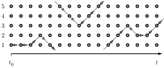
Figure 1: A Markov chain on a five-site lattice with periodic boundary conditions. The particle hops from a site $k$ towards its neighbors with probability $1/3$ each.

The equal hopping probabilities imply via the detailed balance condition

$$\pi_{k}p_{k\to l}=\pi_{l}p_{l\to k}$$ (4)

that the stationary probability distribution $\pi_{k}=1/N$ of this problem is independent of $k$.

This system’s Monte Carlo algorithm is encoded in the $N\times N$ transfer matrix $T^{1,1}$:

$$T^{1,1}=\{p(i\to j)\}=\frac{1}{3}\begin{pmatrix}1&1&0&\cdots&0&1\\ 1&1&\ddots&&\cdots&0\\ 0&\ddots&\ddots&\ddots&&\vdots\\ \vdots&&\ddots&\ddots&\ddots&0\\ 0&\cdots&&\ddots&1&1\\ 1&0&\cdots&0&1&1\\ \end{pmatrix}.$$ (5)

The eigenvalues of $T^{1,1}$ are $\lambda^{1,1}_{k}=\frac{1}{3}\left(1+2\cos{\frac{2(k-1)\pi}{N}}\right),k=1,\ldots,\text{Int}[N/2]+1$ (with multiplicities) that is, for $N=5$, $\{1,\frac{1+\sqrt{5}}{6},\frac{1-\sqrt{5}}{6}\}$. The largest eigenvalue, $\lambda^{1,1}_{1}=1$ corresponds to the conservation of probabilities. By construction, it is associated with the equilibrium solution $(\pi_{1},\ldots,\pi_{N})=(\frac{1}{N},\ldots,\frac{1}{N})$. The second-largest eigenvalue is $\lambda^{1,1}_{2}$. For $N=5$ we have $\lambda^{1,1}_{2}=\frac{1+\sqrt{5}}{6}=0.539$. This eigenvalue controls the long-time corrections to the stationary solution, which vanish as $[\lambda^{1,1}_{2}]^{t}=\exp\left[-t/\tau_{\text{corr}}\right]$, with

$$\tau_{\text{corr}}=1/|\log\left(\lambda^{1,1}_{2}\right)|.$$

We note that the time scale $\tau_{\text{corr}}$ only describes the asymptotic behavior of the correlation. The calculation of the time $t$ at which the probability distribution $\pi^{t}$ itself is within a suitably chosen $\epsilon$ of a the equilibrium distribution $\pi$ is more involved (see, for example, perez ; diaconis ).

II.1 Coupling

As illustrated in Fig. 2, the Monte Carlo algorithm can be formulated in terms of random maps. In our example, this means that instead of prescribing one move per time step, as in Fig. 1, we now sample moves for all times $t$ and all sites $k$, in such a way that the dynamics of a single particle again satisfies the detailed balance condition of Eq. (4). The most natural implementation of this approach is illustrated in Fig. 2: arrows are chosen independently for all times $t$ and all sites $k$. At time $t_{0}$, for example, the particle should move down from sites $1$, $3$, $4$ and $5$ and straight from site $2$. We can now check the outcome of the Monte Carlo calculation. In the example of Fig. 2, from time $t_{0}+10$ on, all initial configurations of the single particle yield the same output. This is remarkable because, evidently, at this time the initial conditions are completely forgotten.

The coupling time $t_{\text{coup}}$ is a random variable ($t_{\text{coup}}=10$ in Fig. 2) which depends on the realization of the full Monte Carlo simulation from time $t_{0}$ onwards (until coupling has been reached). The independence of random maps on different time steps implies that the probability for not coupling vanishes at least exponentially fast in the limit $t\to\infty$.

Under the random-map dynamics, an initial state with $N$ particles eventually evolves into a state with one particle (in later sections, spin-glass configurations will take the place of the single-particle positions). More generally, a state with $k$ configurations can evolve at each time step into a state with $k^{\prime}\leq k$ configurations. Figure 2 displays a sequence of random maps and illustrates the associated time-forward search of the coupling time.

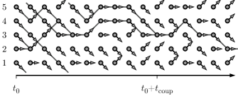
Figure 2: Extended Monte Carlo simulation on $N=5$ sites. Trajectories from all possible initial configurations at $t=t_{0}$ are indicated. They “couple” at $t=t_{0}+t_{\text{coup}}$. The coupling time (here $t_{\text{coup}}=10$) depends on the realization of the Markov chain.

This extended Monte Carlo dynamics on $k$-configuration states can again be described by a transfer matrix:

$$T^{\text{fw}}=\begin{pmatrix}T^{1,1}&T^{2,1}&\dots&&\dots\\ 0&T^{2,2}&T^{3,2}&&\dots\\ 0&0&T^{3,3}&&\dots\\ \dots&&&\ddots&\\ 0&0&&&T^{N,N}\\ \end{pmatrix},$$ (6)

where the block $T^{k,l}$ (of sizes $\binom{N}{k}\times\binom{N}{l}$) concerns all the processes which lead from a state at time $t$ with $k$ configurations to a state with $l\leq k$ configurations at time $t+1$. The upper left block of this matrix, $T^{1,1}$, is the original matrix from Eq. (5). As an example, we find from Eq. (3) the following elements of this transfer matrix:

$$T^{\text{fw}}\{|\circ\circ\bullet\circ\!\ \bullet\rangle \to|\circ\bullet\circ\bullet\!\ \circ\rangle\}=1/9$$

$$T^{\text{fw}}\{|\circ\circ\bullet\circ\!\ \bullet\rangle \to|\circ\circ\circ\bullet\!\ \circ\rangle\}=1/9$$

$$T^{\text{fw}}\{|\circ\circ\bullet\bullet\!\ \bullet\rangle \to|\circ\circ\circ\bullet\!\ \circ\rangle\}=1/27,$$

etc. The matrix $T^{\text{fw}}$ describes a physical system with variable particle number (from $1$ to $N$) and a space comprising $2^{N}-1$ states, the number of non-empty states in this new simulation (for a problem of $N$ spins, the number of configurations is $2^{N}$ and the total number of $k$-configuration states (states with $k$ configurations) is $2^{2^{N}}-1$).

Figure 3: The exact probability that the Markov chains have not coupled by time $t$ (computed by repeated application of the forward transfer matrix), compared to the time-scales $\tau_{\text{corr}}$, $\tau_{\text{coup}}$, and $\tau^{*}$ (One-dimensional diffusion model with $N=5$).

The “forward” transfer matrix $T^{\text{fw}}$ allows us to compute the coupling probabilities as a function of time in Fig. 3. The matrix $T^{\text{fw}}$ is block-triangular in the number of particles $(k,l)$, with the $(1,1)$ block given by $T^{1,1}$. Therefore, all the eigenvalues of $T^{1,1}$ are also eigenvalues of $T^{\text{fw}}$. In particular, the largest eigenvalue of $T^{\text{fw}}$ is again $\lambda^{\text{fw}}_{1}=1$, with corresponding right eigenvector $\tfrac{1}{5}(|\bullet\circ\circ\circ\!\ \circ\rangle+\cdots+|\circ\circ\circ\circ\!\ \bullet\rangle)$. The second-largest eigenvalue of $T^{\text{fw}}$ belongs to the $(2,2)$ block and leads to the time scale of the coupling, $\tau_{\text{coup}}$. It is given by $\lambda^{\text{fw}}_{2}=0.838$, larger than $\lambda^{\text{MC}}\equiv\lambda_{2}^{1,1}$. This second-largest eigenvalue $\lambda^{\text{fw}}_{2}$ governs the coupling probability $\mathcal{P}(t_{\text{coup}})$ for large times. It follows from the block-triangular form of the forward transfer matrix $T^{\text{fw}}$ that the time scales satisfy $\tau_{\text{coup}}\geq\tau_{\text{corr}}$. A general argument allows us to better understand this result: for any running time $t$ we may separate all the Markov chains into those that have already coupled and those that have not. Only the non-coupled chains (whose number vanishes as $\exp\left(-t/\tau_{\text{coup}}\right)$) contribute to connected correlation functions:

$$\exp\left(-t/\tau_{\text{corr}}\right)\propto\left\langle\mathcal{O}(t)\mathcal{O}(0)\right\rangle=\sum_{\text{config. $\sigma_{t},\sigma_{0}$}}\mathcal{P}(t_{\text{coup}}>t,\sigma_{t},\sigma_{0})\mathcal{O}(\sigma_{0})\mathcal{O}(\sigma_{t})\\ +\sum_{\text{config. $\sigma_{0}$}}\pi^{0}(\sigma_{0})\mathcal{O}(\sigma_{0})\sum_{\text{config. $\sigma_{t}$}}\mathcal{P}(t_{\text{coup}}\leq t,\sigma_{t})\mathcal{O}(\sigma_{t}).$$

Here, $\mathcal{O}$ is an observable whose mean value is zero and $\sigma_{t}$ the configuration of the system at time $t$. For the chains which have coupled by the time $t$, $\sigma_{t}$ does not depend on $\sigma_{0}$, and the contribution to the correlation function vanishes. For the other chains, we find

$$\exp\left(-t/\tau_{\text{corr}}\right)=\sum_{\text{config. $\sigma_{t},\sigma_{0}$}}\mathcal{P}(t_{\text{coup}}>t,\sigma_{t},\sigma_{0})\mathcal{O}(\sigma_{0})\mathcal{O}(\sigma_{t})\propto\exp\left(-t/\tau_{\text{coup}}\right)\exp\left(-t/\tau^{*}\right),$$ (7)

where we suppose that even the non-coupled chains converge towards equilibrium on a time scale $\tau^{*}$, and use that the probability for a chain not to have coupled behaves as $\exp\left(-t/\tau_{\text{coup}}\right)$ in the long-time limit. Equation (7) shows that the difference between $\tau_{\text{coup}}$ and $\tau_{\text{corr}}$ is caused by the convergence taking place within non-coupling chains:

$$\frac{1}{\tau_{\text{corr}}}=\frac{1}{\tau_{\text{coup}}}+\frac{1}{\tau^{*}}.$$ (8)

This relation is illustrated in Fig. 3 for the one-dimensional diffusion model with $N=5$. A later figure, Fig. 8, will illustrate for the case of spin glasses the split between the general spin–spin correlation function and that same object computed for non-coupling chains only.

II.2 Forward and backward coupling

The probability distribution of coupling times in the forward direction can be obtained from the transfer matrix $T^{\text{fw}}$ as we discussed in Section LABEL:s:coupling. Here we analyze the distribution of coupling times in the backward direction for the application of the “coupling from the past” protocol which, as we will see, is the same as the one in the forward direction. The backward coupling process leads to a generalized transfer matrix, $T^{\text{bw}}$, which again describes an extended Monte Carlo simulation.

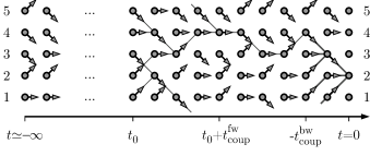
Figure 4: Extended simulation on $N=5$ sites. The outcome of this simulation, from $t=-\infty$ up to $t=0$, is $k=2$. It can be obtained by backtracking from time $t=0$ to $-t_{\text{coup}}^{\text{bw}}$, or by forward simulation from any $t_{0}\leq-t_{\text{coup}}^{\text{bw}}$, through the indicated trajectories. Backtracking from sites $1,3,4$ and $5$ leads to dead ends.

We consider a hypothetical simulation which has run since time $t=-\infty$ up to time $t=0$ (see Fig. 4). It follows from the discussion in Section LABEL:s:coupling that the simulation has coupled. Furthermore, because of the infinite separation between the infinitely remote initial condition and the final one, the resulting configuration (at $t=0$) is in equilibrium. But it remains to be seen which one of the five configurations at $t=0$ is generated. In the example of Fig. 4, a one-step backtrack to time $t=-1$ allows us to see that the configuration at $t=0$ can be neither $k=1$ nor $k=3$ nor $k=5$. Likewise, for $N-1$ output positions on the $N$-site ring this back-propagation leads to a dead end, and only a single position yields a full set of possibilities at some time $-t_{\text{coup}}^{\text{bw}}$. Thus to find the output configuration of the simulation, one is interested in the first time in the past for which the simulation couples, that is one searches the “backward” coupling time. The implementation of this backward simulation, as defined for many particles, can again be described by a transfer matrix. For any distribution of arrows, any occupied site $k$ at time $t$ propagates its occupation back to all the sites at time $t-1$ which have arrows pointing towards $k$. The matrix element of $T^{\text{bw}}$ between two states is given by the statistical weights of all the arrows connecting the two states. For example, we find for $T^{\text{bw}}$

$$T^{\text{bw}}\{|\circ\circ\bullet\circ\!\ \circ\rangle \to|\circ\bullet\bullet\circ\!\ \circ\rangle\}=4/81$$

$$T^{\text{bw}}\{|\bullet\bullet\circ\bullet\!\ \bullet\rangle \to|\bullet\circ\circ\bullet\!\ \bullet\rangle\}=4/81$$ (9)

$$T^{\text{bw}}\{\underbrace{|\circ\circ\bullet\circ\!\ \bullet\rangle}_{\text{time $t$}}\} \to\underbrace{|\circ\circ\circ\bullet\!\ \circ\rangle}_{\text{time $t+1$}}\}=2/27.$$

This is a non-trivial variant of the forward simulation as, for example, the matrix $T^{\text{bw}}$ is not block-triangular as $T^{\text{fw}}$, but it is particle–hole symmetric (as we see in the above example).

Formally, a random map $f$ (here a set of arrows) associates configurations which are connected under the Monte Carlo dynamics. A $k$-configuration state $|x\rangle$ is by definition a set of configurations. At time $t$ the state $|x\rangle$ can be associated with the state $|y\rangle$ at time $t+1$ via the forward matrix if and only if $|y\rangle$ is the (set) image of $|x\rangle$ by an allowed mapping $f$ (i.e. $|y\rangle=f(|x\rangle)$). The same holds for the backward matrix but $|x\rangle$ must be the reciprocal (set) image of $|y\rangle$ (i.e. $|x\rangle=f^{-1}(|y\rangle)$). The backward transfer matrix $T^{\text{bw}}$ manifestly differs from the forward matrix $T^{\text{fw}}$. However, we construct explicitly in Appendix LABEL:s:similarity the similarity transform that maps $T^{\text{fw}}$ onto $T^{\text{bw}}$. This means that

$$PT^{\text{fw}}=T^{\text{bw}}P.$$

(see Appendix LABEL:s:similarity). The similarity transformation $P$ associates a $k$-configuration state $|x\rangle$ with the sum of states that share at least one configuration with $|x\rangle$, included itself. The spectrum of the backward transfer matrix thus agrees with the one of the forward matrix and the distribution of coupling times $\mathcal{P}(t_{\text{coup}})$ is identical for backward and forward dynamics. This result is natural because the probabilities for not coupling for $t$ time steps are identical in both forward and backward direction: $\mathcal{P}(t_{\text{coup}}^{\text{bw}}>t)=\mathcal{P}(t_{\text{coup}}^{\text{fw}}>t)$ (see read_once ). The probability distribution $\mathcal{P}(t=t_{\text{coup}}^{\text{bw}})$ measures the weight of the configuration $|\bullet\bullet\bullet\bullet\!\ \bullet\rangle$ under repeated application of the backward transfer matrix from the configuration at $t=0$: $|\bullet\circ\circ\circ\!\ \circ\rangle+\cdots+|\circ\circ\circ\circ\!\ \bullet\rangle$.

II.3 Choice of random maps

Transition probabilities of the forward transfer matrix must satisfy the Markov chain transition probabilities for single particles, but the choice of random maps is otherwise unrestricted. The one-particle sector is trivially correct for independent moves as in our diffusion model of Section LABEL:s:coupling. We now discuss several alternative random maps for the one-dimensional diffusion, which may lower (or increase) the coupling time (with, however $\tau_{\text{coup}}\geq\tau_{\text{corr}}$) or achieve a rapid reduction of the number of configurations for smaller time scales.

A naive example for the one-dimensional diffusion example consists of arrows, such as in Fig. 2, but which for one time $t$ all point into the same direction, straight, up, and down, each with probability $1/3$, so that single-particle moves satisfy the detailed balance condition. Evidently, this random map does not couple, and the non-coupling Markov chains, in Eq. (8), converge in a time $\tau^{*}=\tau_{\text{corr}}$. We now modify this rigid algorithm by allowing arrows to change direction with probability $\epsilon$. This makes the Markov chain couple on a time scale $\sim\log{\frac{1}{\epsilon}}$, much larger than the correlation time $\tau_{\text{corr}}$, for small $\epsilon$. The choice of independent random moves ($\epsilon=1$) is optimal in this class of maps, but it is not the choice minimizing $\tau_{\text{coup}}$ among all random maps. For example we may choose correlated moves for selected neighboring pairs of sites say, for sites $(1,2)$ and $(3,4)$ and let the move from site $5$ be independent (see Fig. 5).

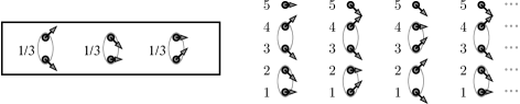
Figure 5: Left: Transition probabilities for pairs $(1,2)$ and $(3,4)$ for the correlated random map. Right: In the extended Monte Carlo simulation shown, the one-particle transition probabilities are as in Fig. 1, but nearest-neighbor coupling is favored.

Elements of $T^{\text{fw,corr}}$ are, for example,

$$T^{\text{fw,corr}}\{|\circ\circ\bullet\bullet\!\ \circ\rangle \to|\circ\circ\bullet\bullet\!\ \circ\rangle\}=0$$

$$T^{\text{fw,corr}}\{|\circ\circ\bullet\bullet\!\ \circ\rangle \to|\circ\circ\bullet\circ\!\ \circ\rangle\}=1/3$$

$$T^{\text{fw,corr}}\{|\circ\circ\bullet\bullet\!\ \circ\rangle \to|\circ\bullet\circ\circ\!\ \bullet\rangle\}=1/3$$

$$T^{\text{fw,corr}}\{|\circ\circ\bullet\bullet\!\ \circ\rangle \to|\circ\circ\bullet\circ\!\ \bullet\rangle\}=0.$$

The single-particle sector of this algorithm is as before, but the second-largest eigenvalue of the transfer matrix $T^{\text{fw}}$ with such correlated pair moves becomes smaller, indicating faster coupling:

$$\lambda_{2}^{1,1}<\lambda^{\text{fw,corr}}_{2}=0.777<\lambda_{2}^{\text{fw,indep}}=0.838.$$

Coupling times of both “independent-arrow” random mapping and “correlated-pair” random mapping scale alike for large $N$. We note that in applications, as in our patch algorithm of Section LABEL:s:local_patch, it might be not so much of interest to speed up the coupling than to rapidly decrease the number of possible configurations at times $t<\tau_{\text{coup}}$. Therefore, one goal could be to decrease the eigenvalues of the matrix $T^{k,k},k\gg 1$, whose time scales correspond to the rapid reduction of the number of configurations towards more manageable numbers.

II.4 Exact sampling, coupling from the past

As discussed in Section LABEL:s:forward_and_backward, the coupling of Markov chains allows one to produce exact samples of the equilibrium distribution: In the diffusion example, we were able to run the Monte Carlo simulation backwards in time using $T^{\text{bw}}$, but this matrix can usually not be constructed. To find the sample at time $t=0$, one may tentatively set a time $t_{0}<t$ and produce all the random maps between time $t_{0}$ and $t$. One can then check explicitly whether all the possible initial conditions at time $t_{0}$ have coupled, that is, for the diffusion problem, whether the initial $N$-particle configuration $|\bullet\bullet\bullet\bullet\!\ \bullet\rangle$ has yielded one of the one-particle configurations. If this goal has not been reached, one must complement the random maps already computed with random maps for earlier times (see Fig. 4). The one-dimensional diffusion problem without periodic boundary conditions illustrates an algorithm which determines the coupling time with much less effort. We consider odd times at which only sites $1,3$ and $5$ and even time steps at which only sites $2$ and $4$ may flip (see Fig. 6). This preserves the correct stationary probability distribution, but the trajectories no longer cross each other (as at time $t_{0}+1$ in Fig. 2). As a consequence, it suffices to follow the two extremal configurations, which start at sites $k=1$ and $k=N$, from time $t_{0}$ on in order to determine the coupling time for a given full Monte Carlo simulation. The multiple-particle Monte Carlo simulation starts with the state $|\bullet\circ\circ\circ\!\ \bullet\rangle$ until it yields a single-particle state. The above strategy of following extremal configurations can be applied to the ferromagnetic Ising model (but not to spin glasses, see propp ; SMAC ). In this case, the two configurations with all spins up and all spins down, respectively, are extremal. This idea also holds for the heat-bath algorithm of two-dimensional directed polymers in a random medium.

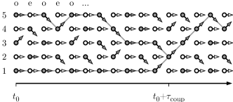
Figure 6: Extended Monte Carlo simulation with odd (o) and even (e) time steps on a lattice without periodic boundary conditions. Trajectories cannot cross, and the coupling of the two extremal initial configurations (the simulations starting at time $t_{0}$ from sites $1$ and $5$) determines the coupling time.

III Coupling and convergence in spin models

We study the Edwards–Anderson $\pm J$ Ising spin glass on a $d$-dimensional square lattice, where each site is randomly coupled to all its $2d$ neighbors. The energy of a configuration $\sigma=(\sigma_{1},\dots,\sigma_{N})$ with $\sigma_{k}=\pm 1$ is:

$$\mathcal{H}(\sigma)=-\sum_{\langle i,j\rangle}J_{ij}\sigma_{i}\sigma_{j},$$

where $\langle i,j\rangle$ indicates the sum over nearest neighbors. This model has a phase transition at finite temperature in $3d$ and at zero temperature in $2d$. Sampling spin-glass configurations with Markov-chain algorithms is extremely difficult in $d=3$ dimensions below the critical temperature, but it is also non-trivial in the two-dimensional case swendsen . We concentrate here on the study of a local heat-bath Monte Carlo algorithm, for which we apply the coupling-from-the-past protocol and obtain exact samples. We note that in two dimensions, the exact partition function of the Ising model on a finite lattice can be determined exactly for any choice of couplings saul ; SMAC . This makes possible a direct-sampling algorithm, which is completely unrelated to the material presented here, but which we sketch, for the sake of completeness, in Appendix LABEL:s:onsager_method.

The heat-bath Monte Carlo algorithm for spin models updates at each time step a randomly chosen site $i$ of a spin configuration by comparing a function of the local field on site $i$ with a uniform random number $\Upsilon_{i}(t)=\text{ran}[0,1]$:

$$\sigma_{i}(t+1)=\begin{cases}1&\text{if}\ \Upsilon_{i}(t)\leq\left[1+\mathrm{e}^{-2\beta h_{i}(t)}\right]^{-1}\\ -1&\text{else}\end{cases},$$ (10)

where $h_{i}(t)=\sum_{j}J_{ij}\boldsymbol{\sigma}_{j}(t)$ is the local field on site $i$. A realization of the Markov chain corresponds to sampling the real-valued random numbers $\{\ldots,\Upsilon(t_{0}),\Upsilon(t_{0}+1),\ldots,\Upsilon(-1)\}$ and the random integers $\{\ldots,i(t_{0}),i(t_{0}+1),\ldots,i(-1)\}$. The unit of “physical” time (one “sweep”) corresponds to $N$ individual updates. The situation is now much more complicated than for the $1d$ diffusion, as the role of the five initial configurations in Fig. 2 is taken up by the $2^{N}$ possible spin configurations. To prove coupling one must show to which configuration they all converge at the coupling time. The state space is huge and one must find strategies to avoid enumerating and surveying $2^{N}$ configurations.

III.1 Partial-survey approximation

In chanal , we presented an exact-sampling algorithm which works down to quite low temperatures in the two-dimensional Ising spin glass, and which is also operational in three dimensions. We found that practically the same results could be obtained by starting the simulation at time $t_{0}$ not from all the $2^{N}$ initial configurations, but from a more manageable number $\mathcal{N}(t_{0})$ of randomly chosen configurations. We show in Fig. 7 that such “partial survey” calculations yield useful lower bounds for the coupling time scale $\tau_{\text{coup}}$. Each curve in the figure represents the mean number of distinct configurations remaining after coupled Monte Carlo simulations (that is, with the same random numbers $(\Upsilon,i)$ for all configurations) for different values of $\mathcal{N}(t_{0})$. Increasing $\mathcal{N}(t_{0})$ within this partial-survey approximation naturally improves the lower bound on the coupling time but, in practice, the value obtained saturates quite quickly.

Figure 7: Number of configurations of the partial survey approximation with $\mathcal{N}(t_{0})$ random initial configurations for the Ising spin glass on a $16\times 16$ lattice at temperature $\beta=0.5$. We average over $10$ choices of $J_{ij}$, and use the same values of $J_{ij}$ and the same random numbers $\Upsilon_{i},i$ for all initial configurations.

III.2 Correlation functions

As discussed previously, $\tau_{\text{coup}}$ is always larger than $\tau_{\text{corr}}$ because only non-coupling chains contribute to correlation functions (see Eq. (8)).

Figure 8: Spin–spin correlation function for all Markov chains and for the non-coupling Markov chains only ($\beta=1$, random initial conditions) (Two-dimensional $8\times 8$ spin glass at $\beta=1$).

To again illustrate the relation between coupling and convergence times, we separate in Fig. 8 non-coupling chains from the calculation of the spin–spin correlation function of a $8\times 8$ spin glass at inverse temperature $\beta=1$. Indeed, even if the chain has not coupled, the configurations $\sigma_{t}$ may lose the dependence on the initial configuration $\sigma_{0}$.

IV Coupling for hard-sphere systems

In this section we discuss the application of the “Coupling from the past” protocol to hard-sphere systems. The study of Monte Carlo algorithms for hard-sphere systems goes back a long time, as the Metropolis algorithm was first implemented for hard disks, that is, two-dimensional spheresmetropolis . Even today, the physics of the hard-disk system is not well understood, and Monte Carlo algorithms have not been developed as successfully as, say, for the Ising model. In this very constrained system, the estimation of correlation times is quite controversial, especially at high densitiesbernard_2009 , and rigorous results from exact-sampling approaches would be extremely welcome.

We first discuss the birth–death formulation of the Markov-chain Monte Carlo algorithm for this system and then compute lower bounds on coupling times using the partial-survey algorithm. Its empirical coupling time saturates (for increasing $\mathcal{N}(t_{0})$) to much smaller values than the coupling times obtained by the summary-state method read_once ; Kendall . This suggests that these previous algorithms are not optimal, an impression which is confirmed by our local-patch algorithm of Section LABEL:s:patch_disk.

The partition function of hard spheres in the grand-canonical ensemble, with fugacity $\lambda$, is given by a weighted sum over legal configurations of spheres:

$$\mathcal{Z}=\sum_{N=0}^{+\infty}\int\!\!d^{2N}\!\sigma^{(N)}~{}\lambda^{N}~{}\ \Theta\left(\sigma^{(N)}\right).$$ (11)

Here, configurations of $N$ spheres are written as:

$$\sigma^{(N)}=\{(x_{1},y_{1}),(x_{2},y_{2}),\ldots,(x_{N},y_{N})\},$$

where $(x_{k},y_{k})$ denotes the centers of the spheres. In Eq. (11), $\Theta(\sigma^{(N)})$ equals one if spheres of the configuration $\sigma^{(N)}$ do no overlap and zero otherwise. We again use periodic boundary conditions.

IV.1 Birth–death algorithm for hard spheres

The spatial Poisson birth–death process allows us to apply coupling from the past to hard-sphere systems (see Kendall ; read_once ): Disks of radius $r$ arrive (“are born”) randomly on a two-dimensional unit square with constant rate $\lambda$. Once born, they disappear (“die”) with unit rate.

The probability for a disk to arrive within an infinitesimal time $dt$ in a small box of area $dS$ centered at $(x,y)$ is $\lambda dtdS$. This disk is added to the configuration only if it overlaps with no other disk present. Each disk disappears with probability $dt$ within the time interval $dt$. Sphere are added at point $(x,y)$ or removed from the configuration $\sigma^{(N)}$ according to the detailed balance condition. With the notation $\sigma^{(N+1)}=\sigma^{(N)}\cup\{(x,y)\}$ we have:

$$\mathcal{P}(\sigma^{(N)}\rightarrow\sigma^{(N+1)})\pi(\sigma^{(N)}) =\lambda~{}\Theta(\sigma^{(N+1)})\pi(\sigma^{(N)})$$

$$=\pi(\sigma^{(N+1)}),$$

$$\mathcal{P}(\sigma^{(N+1)}\rightarrow\sigma^{(N)})\pi(\sigma^{(N+1)}) =1\times\pi(\sigma^{(N+1)}).$$

In Fig. 9, we illustrate the time-evolution of accepted and rejected birth-death events on a one-dimensional hard-sphere problem, starting from an empty initial condition at time $t_{0}$.

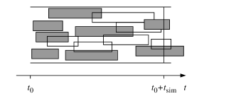
Figure 9: Simulation of the birth–death algorithm for one-dimensional “spheres” in a box. The simulation starts at time $t_{0}$ and stops at $t_{0}+t_{\text{sim}}$ with $N=2$ spheres. Transparent spheres are rejected because they overlap with spheres already present.

In the hard-sphere algorithm, the probability distribution of time intervals between successive births is an exponential with parameter $\lambda$: $\mathcal{P}(\tau_{b})=\lambda e^{-\lambda\tau_{b}}$. In Fig. 9, the life time of a sphere is represented by a horizontal extension of the box, irrespective of whether it has been accepted or not (the vertical dimension denotes the diameter). Life times are exponentially distributed as well. For the exponential distribution, the time before the next death of a system of $N$ spheres follows an exponential distribution with parameter $N$. Likewise the time before any event, (birth or death), follows an exponential distribution with parameter $\lambda+N$. The probability for the next event to be a birth is then $\frac{\lambda}{\lambda+N}$.

IV.2 Coupling and partial survey approximation

Coupling from the past applies to hard-sphere systems even though the space of configurations is continuous (unlike in lattice simulations). To apply the protocol, one considers a time evolution, as in Fig. 9, but stretching back to time $t=-\infty$. Two special aspects must now be handled:

First, we must determine which boxes (corresponding to spheres) are indeed placed (“True”), and which ones are rejected (“False”). This is difficult to decide at high density. However, in the low-density case presented in Fig. 10, several spheres are “True”, simply because they do not overlap with already present “True” or “False” spheres. This allows the status of other spheres to be fixed and, finally, the configuration to be constructed. In the limit $N\to\infty$, the approach works up to a constant density luby . This density is much higher than the density $\propto 1/N$ direct-sampling algorithm can achieveSMAC . This approach Kendall ; read_once is equivalent to deciding whether a given spin is up or down in the “summary state” algorithm for Ising systems huber ; Childs , which, in the thermodynamic limit works down to a fixed constant temperature.

Second, one must fix the initial condition at time $-T$, because spheres born at times smaller than $-T$ may still be alive at time $-T$. This is solved through the sampling of a second time, $T_{\text{start}}$, after which we know that all spheres present at time $-T$ have disappeared. The time interval $T_{\text{start}}+T$ is sampled as the maximum of $N_{\max}$ life times, where $N_{\max}$ is an upper bound on the number of spheres in a legal configuration.

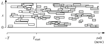
Figure 10: Time evolution of a one-dimensional birth–death simulation in a box of size $L$. All spheres correspond to rectangles whose horizontal extension indicates their life time. From any possible cut of “True” boxes at $T_{\text{start}}$ ($7$ boxes actually cut the line, so there are $\leq 2^{7}$ possible cuts) one can deduce the output at time $t=0$, as in Fig. 9.

Figure 10 sketches the time evolution of a Monte Carlo simulation for the one-dimensional hard-sphere problem which has started at time $t=-\infty$. Boxes are drawn starting from time $-T$, but the simulation is picked up at time $T_{\text{start}}$. It is straightforward to complement the simulation shown (between times $-2T$ and $-T$, for example), in case it does not couple in the interval shown. However, we must show that it couples between $-2T$ and $-T$ or at least results in less than $N_{\max}$ spheres. In the Monte Carlo simulation in Fig. 10, the status of the boxes at later times can be easily decided, because at later times all spheres belong to clusters which are disjoint from the initial condition. However, this possibility disappears at higher densities. A simple example of this is shown in Fig. 11. As one cannot decide on the status of the initial sphere (which crosses the line at $T_{\text{start}}$), we should initialize the simulation with the two configurations, one corresponding to a “True” state and one to a “False” state. After several steps of the time evolution, we arrive in both cases at the same physical configuration (the two dark spheres, which are both “True”).

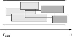
Figure 11: Example of a time evolution of the one-dimensional birth–death simulation which where no single sphere can be decided independently. Starting with all possible choices of the initial configuration at $t=T_{\text{start}}$ allows to prove coupling. (The two dark spheres are “True”, while the transparent sphere must be “False”.)

For all times $t>T_{\text{start}}$, we consider the set $\mathcal{C}(t)$ of all “True” or “False” spheres crossing the time line at $t$ (see Fig. 10). From the set $\mathcal{C}$, one can in principle construct all the possible initial configurations, but their number remains huge. As in the spin-glass case, we may also select $\mathcal{N}(T_{\text{start}})$ among these configurations, and propagate these. This is again the partial survey approximation. In Fig. 12 we compare average lower bounds on the coupling time from this approximation with results from the summary state algorithmread_once . In the time-evolution of Fig. 10, one can determine the number of remaining configurations at any time $t>T_{\text{start}}$ and detect when exactly the coupling occurs.

Figure 12: Coupling times of the summary-state algorithm for hard disks Kendall ; read_once compared to the local-patch algorithm. Lower bounds are provided by the partial-survey approximation. The disks’ radius is $r=0.04$ in a unit square box with periodic boundary conditions, so that there are $\sim 60$ disks at density $\eta=0.3$.

V Local-patch algorithm

In the present section, we discuss our local-patch algorithm, which performs the heat-bath dynamics for a general $d$-dimensional Ising spin glass on an $N$-site hyper-cubic lattice. This algorithm allows us to control all the $2^{N}$ initial configurations even for very large lattices and to eventually prove that the system has coupled. The Python script implementing this algorithm has less than 300 lines. It is available electronically and a listing of the code is contained in Appendix LABEL:s:listing_python.

V.1 Patches

The (non-rigorous) partial-survey algorithm of Section LABEL:s:partial_survey determines the coupling time for a subset of all the configurations at time $t$. The (rigorous) patch algorithm, in contrast, works with a superset of all configurations at time $t$: by restricting the configurations to the smaller region of a patch, one severely limits their number, at the price of introducing compatibility problems between neighboring patches. For the two-dimensional spin glass, we use $N$ rectangular patches of same shape and orientation, with $M$ sites, and initially at $t=t_{0}$, we have $2^{M}$ spin configurations on each patch. Likewise, the set of global spin configurations is broken up into a list $[S_{1}(t),\ldots,S_{N}(t)]$ of sets $S_{k}(t)$ of spin configurations restricted to patches $k$. We can recover a superset $\Omega(t)$ of all relevant spin configurations from the direct product

$$\Omega(t)=S_{1}(t)\otimes S_{2}(t)\otimes\cdots\otimes S_{N}(t)/\text{(compat)}.$$ (12)

Here, each configuration of $\Omega(t)$ is pieced together from configurations on all patches, with compatible spins on all lattice sites. (Two compatible spin configurations, on patches $k$ and $l$, are shown in Fig. 13). On large lattices, the direct product in Eq. (12) can be performed only if the number of spin configurations per patch is small. If there is only one configuration per patch, we can construct a unique global configuration on the whole lattice.

For each time step $t$ of the heat-bath algorithm, we choose a random lattice site $i$ and a random number $\Upsilon=\text{ran}[0,1]$ and then update the spin $\sigma_{i}$ for all configurations on all patches containing $i$. The site $i$ may be in the center of a patch $k$ (all the neighbors of site $i$ also belong to $k$, as in Fig. 13). In this case, each configuration of $S_{k}(t)$ yields one configuration of $S_{k}(t+1)$. Several configurations in $S_{k}(t)$ may yield the same configuration in $S_{k}(t+1)$, so that the size of $S_{k}$ does not increase in this case. If the site $i$ is on the boundary of a patch $l$, we only know upper and lower bounds for the field on the site $i$ and, depending on the value of the random number $\Upsilon$, may be unable to update $\sigma_{i}$. In this case, we add two configurations to the set $S_{k}(t+1)$, corresponding to $\sigma_{i}=-1$ as well as $\sigma_{i}=+1$. The set $S_{k}(t+1)$ may then contain more configurations than $S_{k}(t)$.

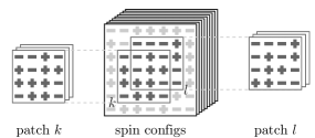
Figure 13: Two patches, $k$ and $l$, with a pair of compatible spin configurations.

V.2 Compatibilities, pruning

Besides updating configurations on patches, we also perform a “pruning” operation: Figure 13 presents two “compatible” configurations on patches $k$ and $l$. These could possibly be pieced together into a global configuration, together with configurations on other patches. On the other hand, if the set $S_{l}$ contains no configuration compatible with a configuration $\boldsymbol{\sigma}$ on patch $k$, we can eliminate (prune) $\boldsymbol{\sigma}$ from $S_{k}$. Pruning may be implemented through a dictionary (hash table), using as “key” the part of the patch configuration in the overlap region between $k$ and $l$, and as “value” the list of patch configurations sharing this key (see Fig. 14). This is programmed very easily in the Python programming language (see Appendix LABEL:s:listing_python).

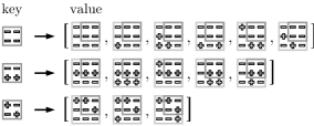
Figure 14: A dictionary (hash table) associating keys (configurations in the overlap region between patches $k$ and $l$) to values (lists of patch configurations with the given key in patch $k$).

Pruning can be iterated until all the sets $S_{k}(t)$ are pairwise compatible. To achieve this goal, it suffices to prune nearest-neighbor patches only. We have found it useful to perform one pruning operation for each pair of nearest-neighbor patches after a certain number of updates (see Fig. 15). The average number of configurations per patch saturates to a value which depends on the temperature and also the size of the patch. This is due to the balance between the decrease of the number of configurations induced by the coupling and its increase caused by the noise at the patch boundaries. This noise is reduced through the crucial pruning step of the algorithm.

Figure 15: Average number of configurations per patch vs. time, at inverse temperature $\beta=1$ in the two-dimensional Ising spin glass on a $16\times 16$ lattice at temperature $\beta=1$. For a given patch size (here $3\times 3$) the number of configurations per patch saturates to a value that depends on the number of prunings per sweep (here: from one to eight). Each pruning is done once for all nearest-neighbor patches.

V.3 Merging of patches

As illustrated in Fig. 15, the number of configurations per patch does not necessarily drop to one at large times, even if the underlying heat-bath dynamics couples. The entropy per spin is smaller for larger patches, because the influence of the boundaries is reduced. However, one cannot start the computation with large patches because of the large number of possible configurations. A merging procedure allows to increase the patch size in a rigorous way. Merging is implemented analogously to pruning: for overlapping patches $k$ and $l$, dictionaries are again computed with the same keys and values (see again Fig. 13). For a given key configuration on the overlap region, we assemble the corresponding values in the dictionary of patch $k$ with all corresponding values in the dictionary of patch $l$. All these couples of configuration must be taken into account for the larger patch $k\cup l$. The merging of the configurations on neighboring patches can be implemented very efficiently in the Python programming language (see Appendix LABEL:s:listing_python). In our computations, we start with small square patches, say of size $3\times 3$, and then pass to the size $4\times 3$, after a few sweeps, then to size $4\times 4$, etc. An analogous procedure is followed in higher dimensions. Results obtained with this “jump-start” approach are shown in Fig. 16 for the two-dimensional Ising spin glass at temperature $\beta=0.5$, with a disorder average performed over about $100$ samples.

Figure 16: Number of configurations per patch for the $32\times 32$ spin glass at temperature $\beta=0.5$. A simulation with constant $3\times 3$ patches is compared to the result of a “jump-start” procedure $3\times 3\to 4\times 3\to 4\times 4\to\dots\to 5\times 5$. All results are averaged over $100$ samples.

V.4 Memory of compatibilities, variants

In the patch algorithm, the pruning procedure detects inconsistent configurations in a particular patch. Two configurations on different patches are considered compatible if their spins match in the overlap region (at time $t$). More generally, we can keep track of the past evolution of patch configurations and may then declare them compatible only if they have matched for all times up to $t$. Otherwise, they cannot belong to a unique global spin configuration.

In chanal , the bipartite nature of the square lattice was used to update one entire sub-lattice at a time. In this approach, only one sub-lattice is stored at a time. This allows one to start with larger patches, but the compatibilities between configurations are less well conserved. By contrast, in the present algorithm, we keep the information on both sub-lattices, and one of the sub-lattices is the past configuration. Two configurations are compatible in this new version if they are compatible on both sub-lattices. Likewise one can use past values of a configuration $\sigma(t)$ to restrict its compatibilities with configurations on other patches.

Other generalizations are more straightforward, one can for example optimize the shape of patches in order to minimize the number of spins on the boundary, and work with more than $N$ patches in order to increase the chance for detecting incompatibilities of configurations.

V.5 Exact sampling for hard spheres with local patches

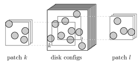
Figure 17: Breaking up disk configurations into patches, with two patches $k$ and $l$ shown.

In this section, we adapt the local-patch algorithm for the classical model of hard disks in a two-dimensional box with periodic boundary conditions. As mentioned, it works for large system sizes at higher density than previous method of exact sampling.

In Section LABEL:s:hard_disk_coup, we introduced the set $\mathcal{C}(t)$ of all disks the dynamics has tried to add in the box and which have not disappeared at time $t$. The coupled Monte Carlo simulations start with all possible configurations that are allowed by the set $\mathcal{C}$ at time $T_{\text{start}}$. Because of possible overlap between disks some of the $2^{\#\mathcal{C}}$ possible configurations are invalid but there may be far too many of them in practice. To reduce the number of configurations which must be handled, we introduce a regular square lattice with $N$ sites covering the simulation box. Likewise, a superset of all feasible configurations on a patch at time $T_{\text{start}}$ can be deduced from the set $\mathcal{C}$, restricted to disks (True or False) with centers inside the patch. From then on, whenever disks appear in the simulation box, we can decide whether they are accepted on a particular patch configuration by checking overlaps into the patch only. Disks that disappear are simply removed from all the concerned patch configurations. At birth time, if the disk to be placed on a patch configuration may overlap with a disk outside the patch, the configuration is split into two: one configuration with the new disk and one without (as for spin systems). To detect and prune irrelevant configurations we check that the updated sets of configurations are compatible with other patches by a pruning procedure analogous to the one of Section LABEL:s:pruning. After several updates, the pruning is performed for most of overlapping patches several times.

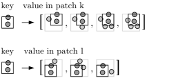
Figure 18: The pruning of a pair of patches via the construction of dictionaries. Each dictionary associates keys (configurations in the overlap region) to values (lists of patch configurations with the given key) (compare with Fig. 14). The merging of patches $k$ and $l$ would lead in this example to $4\times 3=12$ configurations on the combined patch.

For any pair of overlapping patches $k$ and $l$, the pruning eliminates patch configurations with are inconsistent with all other configurations on a neighboring patch. As in the spin glass case, this process can be implemented with dictionaries (hash tables) (see Fig. 18) and can be used to merge configurations on neighboring patches into larger local configurations.

Figure 12 displays the mean coupling times of a hard-disk birth–death simulation for several choices of the fugacity $\lambda$. The radius of the disks is $r=0.04$ in a unit square box with periodic boundary conditions. Results are compared to the partial-survey approximation algorithm, with $\mathcal{N}(T_{\text{start}})=1000$ initial configurations and to the results of the summary-state algorithm.

We concentrated on determining the coupling times of the birth–death dynamics for hard disks. However, the regime of operation of this algorithm is far in the liquid phase (see Fig. 12), and the physically interesting regime, around the liquid–solid transition density, $\eta\simeq 0.71$ SMAC is still out of reach for exact sampling methods. For hard disks, it remains a challenge to set up a working partial-survey algorithm with correlation times comparable to those of the usual Metropolis algorithm bernard_2009 .

VI Conclusion

In this paper, we have discussed exact-sampling algorithms which allow one to totally eliminate the influence of the initial condition from a Markov-chain Monte Carlo simulation. This overcomes one of the main limitations of the method, namely the rigorous estimation of the correlation time. We discussed central subjects, such as the relation between coupling times and convergence times, in a simple example of one-dimensional diffusion, before applying them to Ising spin glasses and to hard-sphere simulations. Algorithmically, the exact-sampling framework obliges one to follow the entire state space of a system. In the absence of simplifications, such as the half-order discussed in Section LABEL:s:coupling_one_d, this can be done approximately through a partial survey of $\mathcal{N}(t_{0})$ initial conditions. One can also restrict the configuration in size onto so-called patches, thereby restricting their number. A superset of the set of global configurations can in principle be reconstituted from the patches. This is easier when the patches are large, and we showed how pruning and merging operations allow one to increase the size of patches during the simulation and to finally prove coupling. Our exact-sampling algorithm works both for spin glasses and hard-disk systems, and were able to go to lower temperatures, and higher densities than previous methods.

The partial survey algorithm, which can be implemented easily, allowed us to prove that our local-patch algorithm is optimal for the local dynamics for both spin-glass and hard-disk systems. We have provided a number of new idea in order to allow exact-sampling methods to reach the phases transitions of the three-dimensional Ising spin glass and the critical density of hard disks.

Appendix A Similarity of forward and backward transfer matrices

Forward and backward transfer matrices completely describe the coupling dynamic of general Markov chains (on a finite state space), that is their elements are the coupled transition probabilities between sets of configurations. Forward and backward matrices represent “extended” Monte Carlo dynamics, in the two time directions. These two formulations are equivalent, even though the forward dynamics, starting from $t=0$, does not generate exact samples. Here, we demonstrate similarity between forward and backward transfer matrices, and construct the similarity transformation between the two.

Let $\Omega$ be the finite space of configurations of the problem of interest. $\Omega$ may contain all $N$ positions on the $N$-site diffusion problem or the $2^{N}$ configurations of a $N$-site spin system.

The $k$-configuration states build up an “extended” state space. They provide a natural basis for the forward and backward matrices. This basis is $2^{\Omega}-\emptyset$, the set of non trivial parts of $\Omega$. For any state $I\in 2^{\Omega}-\emptyset$ we define $\tilde{I}$ as the set of states of the basis $J$ that has at least one configuration in common with $I$ ($J\in\tilde{I}\Leftrightarrow I\cap J\neq\emptyset$). The similarity matrix $P$ is then defined as:

$$P|I\rangle:=\sum_{J\in\tilde{I}}|J\rangle$$ (13)

A random mapping—arrows for the case of 1$D$-diffusion—is a mapping on $\Omega$: $f:\Omega\rightarrow\Omega$. It defines a time step of the Markov chain for every configuration and satisfies $\mathcal{P}(f(i)=j)=p(i\rightarrow j)$ and its weight is noted $w(f)$. In the case of 1$d$-diffusion with independent arrows, or any “independent” random map in general, we naturally define the weight of the random map as a product of elements of the Monte Carlo transfer matrix as

$$w(f)=\Pi_{i\in\Omega}p(i\rightarrow f(i)).$$

The forward matrix associates any state $I$ to all states that it is connected to by a mapping:

$$T^{\text{fw}}|I\rangle=\sum_{f\ \text{rand. map}}w(f)|f(I)\rangle.$$

Using Eq. (13) we find

$$P\ T^{\text{fw}}|I\rangle=\sum_{f\ \text{rand. map}}w(f)\sum_{J\in\tilde{f(I)}}|J\rangle.$$ (14)

The backward matrix $T^{\text{bw}}$ has different rules but we will show that the similarity $P\ T^{\text{fw}}=T^{\text{bw}}P$ holds. Using a random map $f$, a state $J$ at time $t$ evolves to another state $K$ at time $t+1$ in the backward process if and only if $f^{-1}(K)=J$. For example in the 1D-diffusion a hole goes to a hole and a particle goes to a particle. Therefore:

$$T^{\text{bw}}|J\rangle=\sum_{f\ \text{rand. map}}w(f)\sum_{K,f^{-1}(K)=J}|K\rangle$$

and finally:

$$T^{\text{bw}}\ P|I\rangle=\sum_{f\ \text{rand. map}}w(f)\sum_{J\in\tilde{I}}\sum_{K,f^{-1}(K)=J}|K\rangle=\sum_{f\ \text{rand. map}}w(f)\sum_{K,f^{-1}(K)\in\tilde{I}}|K\rangle.$$ (15)

In fact Eqs (15) and (14) are equivalent because $f^{-1}(K)$ overlaps $I$ if and only if $K$ overlaps $f(I)$ ($f^{-1}(K)\cap I\neq\emptyset\Leftrightarrow K\cap f(I)\neq\emptyset$). This proves the similarity of the backward and forward matrices.

Appendix B Exact sampling of two-dimensional spin glass using analytic solution.

In this appendix, we sketch for completeness an unrelated direct-sampling algorithm for the two-dimensional Ising spin glass. To generate exact samples, this algorithm does not use Markov chains. It rather relies on the fact that the partition function of the two-dimensional Ising model or of one sample of the spin glass on a planar lattice with $N$ sites can be expressed as the square root of the determinant of one $4N\times 4N$ matrix (for open boundary conditions) or of four such matrices (for periodic boundary conditions) saul . This relation has been much used in the recent literature, in order to study the physics of the two-dimensional Ising spin glass at low temperature loebl ; marinari . The partition function yields the thermodynamics of the system, but the knowledge of entire configurations gives for example access to complicated spatial configuration functions.

The sampling algorithm for two-dimensional spin-glass configurations constructs the sample one site after another. Let us suppose that the gray spins in the left panel of Fig. 19 are already fixed, as shown. We can now set a fictitious coupling $J_{ll}^{*}$ either to $-\infty$ or two $+\infty$ and recalculate the partition function $Z_{\pm}$ with both choices. The statistical weight of all configurations in the original partition function with spin “$+$” is then given by

$$\pi_{+}=\frac{Z_{+}\exp\left(\beta J_{kl}\right)}{Z_{+}\exp\left(\beta J_{kl}\right)+Z_{-}\exp\left(-\beta J_{kl}\right)}.$$ (16)

and this two-valued distribution can be sampled with one random number. Equation (16) resembles the heat-bath algorithm of Eq. (10), but it is not part of a Markov chain: After obtaining the value of the spin on site $k$, we keep the fictitious coupling, and add more sites. Going over all sites, we can generate direct spin-glass samples at any temperature. We note that this algorithm is polynomial, and the effort is basically temperature-independent, both for the two-dimensional Ising model and the Ising spin glass (see also Krauth09 ).

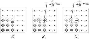
Figure 19: One iteration in the direct-sampling algorithm for the two-dimensional Ising model. The probabilities $\pi(\sigma_{k}=+1)$ and $\pi(\sigma_{k}=-1)$ (with $k$ the central spin) are obtained from the exact solution of the Ising model with fictitious couplings $J_{jk}^{*}=\pm\infty$.

Appendix C Listing of Python code

The following Python code has produced all the spin-glass data presented in this article. An analogous program was used for the hard-disk system. An electronic version of the code is available from the authors.

Algorithm 1: pruning-ND.py

⬇

1#!/usr/bin/python

2##———————————————————————

3## PROGRAM : pruning_ND.py

4## PURPOSE : This program performs the heat-bath and the pruning on a

5## N-dimensional hypercubic lattice with periodic boundary

6## conditions and with cuboid patches.

7## Version with jump-start capability.

8## OUTPUT : mean number of configurations per patch vs. time

9## (can be modified)

10## VERSION : 04-OCT-2009

11## AUTHOR : W. Krauth, C. Chanal

12## LANGUAGE: Python 2.5

13##———————————————————————

14from random import uniform, randint, seed, shuffle, choice

15from operator import itemgetter

16import time, math, os, sys

17##———————————————————————

18## Sample geometry

19##———————————————————————

20def torus_neighbors(N_dim,L):

21 N = L**N_dim

22 site_dic = {}

23 coord_dic = {}

24 for j in range(N):

25 j_d = j

26 x_d = j//(L**(N_dim-1))

27 coord = [x_d]

28 for d in range(N_dim-1): # this loop does not run anything for N_dim=1

29 j_d = (j_d-x_d*L**(N_dim-d-1))

30 x_d = j_d//(L**(N_dim-d-2))

31 coord.append(x_d)

32 coord.reverse() # optional, to set the usual order of the directions

33 coord=tuple(coord)

34 site_dic[coord] = j

35 coord_dic[j] = coord

36 nbr = []

37 for j in range(N):

38 coord = list(coord_dic[j])

39 nbr_list = []

40 for d in range(N_dim):

41 coord[d] = (coord[d]+1)%L

42 coord_p = tuple(coord)

43 nbr_list.append(site_dic[coord_p])

44 coord[d] = (coord[d]-1+L)%L

45 for d in range(N_dim):

46 coord[d] = (coord[d]-1+L)%L

47 coord_p = tuple(coord)

48 nbr_list.append(site_dic[coord_p])

49 coord[d] = (coord[d]+1)%L

50 nbr_list = tuple(nbr_list)

51 nbr.append(nbr_list)

52 nbr = tuple(nbr)

53 return nbr,site_dic,coord_dic

54##———————————————————————

55## Initial patch geometry

56##———————————————————————

57def patch_set(N_dim,L,M,site_dic,coord_dic):

58 patch = []

59 for j in range(N):

60 coord = list(coord_dic[j])

61 dummy_list = []

62 for k in range(M**N_dim):

63 coord_p = []

64 for d in range(N_dim):

65 l = (k//(M**d))%M

66 coord_p.append((coord[d]+ l)%L)

67 coord_p = tuple(coord_p)

68 dummy_list.append(site_dic[coord_p])

69 patch.append(tuple(dummy_list))

70 patch = tuple(patch)

71 return patch

72##———————————————————————

73## Neighbor relations on patches

74##———————————————————————

75def nbr_patch_set(example_patch,nbr):

76 nbr_patch = []

77 for j in example_patch:

78 dummy = []

79 for k in nbr[j]:

80 if k in example_patch: dummy.append(example_patch.index(k))

81 dummy = tuple(dummy)

82 nbr_patch.append(dummy)

83 nbr_patch = tuple(nbr_patch)

84 return nbr_patch

85##———————————————————————

86## Initial patch configurations

87##———————————————————————

88def patch_init(patch):

89 def bin(n,conf_length):

90##

91## convert n to binary number with conf_length digits

92##

93 q = -1

94 bin_conf = ”

95 n_digits = 0

96 while q != 0:

97 q = n//2

98 r = n%2

99 bin_conf = ‘r‘+bin_conf

100 n = q

101 n_digits = n_digits+1

102 n_digits = conf_length-n_digits

103 for i in range(n_digits):

104 bin_conf = ‘0‘+bin_conf

105 return bin_conf

106 configs = []

107 dummy_list = []

108 number = len(patch[0])

109 for j in range(2**number):

110 x = bin(j,number)

111 dummy_list.append(x)

112 for i in range(len(patch)):

113 configs.append(set(dummy_list))

114 return configs

115##———————————————————————

116## Updating configurations on all patches

117##———————————————————————

118def confs_update(N_dim,configs,nbr_patch,Jij,patch,i_site,Upsilon):

119 for k in range(N):

120 if i_site in patch[k]:

121 dummy = list(patch[k])

122 pos=dummy.index(i_site)

123 llist = [patch[k][x] for x in nbr_patch[pos]]

124 Jij_list = [Jij[(i_site,m)] for m in llist]

125 config_k = configs[k]

126 config_kp = set([])

127 for c in config_k:

128 field_char = itemgetter(*nbr_patch[pos])(c)

129 field_sum = sum((2*eval(m)-1)*J for (m,J) in zip(field_char,Jij_list))

130 field_min = field_sum-2*N_dim+len(field_char)

131 field_max = field_sum+2*N_dim-len(field_char)

132 b_one = c[:pos]+’1’+c[pos+1:] # configuration with ’1’ at position ’pos’

133 b_zero = c[:pos]+’0’+c[pos+1:] # configuration with ’0’ at position ’pos’

134 if Upsilon < phplus[field_min]:

135 config_kp.add(b_one)

136 elif Upsilon > phplus[field_max]:

137 config_kp.add(b_zero)

138 else:

139 config_kp.add(b_zero)

140 config_kp.add(b_one)

141 configs[k] = config_kp

142 return configs

143##———————————————————————

144## Pruning of two patches

145##———————————————————————

146def prune_pair(config_k,config_l,KEY_k,KEY_l):

147 f = itemgetter(*KEY_k)

148 Dic_k = {}

149 for x in config_k:

150 a = f(x)

151 if Dic_k.has_key(a): Dic_k[a].add(x)

152 else: Dic_k[a] = set([x])

153 set_k = set(Dic_k.keys())

154 f = itemgetter(*KEY_l)

155 Dic_l = {}

156 for x in config_l:

157 a = f(x)

158 if Dic_l.has_key(a): Dic_l[a].add(x)

159 else: Dic_l[a] = set([x])

160 set_l = set(Dic_l.keys())

161 set_kl = set.intersection(set_k,set_l)

162 config_k = set()

163 config_l = set()

164 for x in set_kl:

165 config_k.update(Dic_k[x])

166 config_l.update(Dic_l[x])

167 return config_k,config_l

168##———————————————————————

169## Merging of two patches

170##———————————————————————

171def merge_pair(config_k,config_l,KEY_k,KEY_l,KEY_add):

172 f = itemgetter(*KEY_k)

173 Dic_k = {}

174 for x in config_k:

175 a = f(x)

176 if Dic_k.has_key(a): Dic_k[a].add(x)

177 else: Dic_k[a] = set([x])

178 set_k = set(Dic_k.keys())

179 f = itemgetter(*KEY_l)

180 Dic_l = {}

181 for x in config_l:

182 a = f(x)

183 if Dic_l.has_key(a): Dic_l[a].add(x)

184 else: Dic_l[a] = set([x])

185 set_l = set(Dic_l.keys())

186 set_kl = set.intersection(set_k,set_l)

187 config_kl = set() #merged set

188 for x in set_kl:

189 for y in Dic_k[x]:

190 for z in Dic_l[x]:

191 zprime = ”.join(itemgetter(*KEY_add)(z))

192 config_kl.add(y+zprime)

193 return config_kl

194##———————————————————————

195## main program starts here

196##———————————————————————

197#seed(13)

198beta =0.25 # inverse of temperature

199##———————————————————————

200## heat bath definitions (see SMAC Fig. 5.20, and SMAC eq. 5.18)

201##———————————————————————

202N_dim = 3

203phplus = {}

204for d in range(N_dim+1):

205 field = 2*d

206 phplus[field] = 1/(1+math.exp(-2*field*beta))

207 phplus[-field] = 1/(1+math.exp(2*field*beta))

208##———————————————————————

209## loop over samples starts here

210##———————————————————————

211L = 6

212os.system(’echo␣‘hostname‘␣‘date‘’)

213print beta, L, ’␣beta␣L’

214for nsamp in range(100):

215 N = L**N_dim

216 M = 2 # M^N_dim is the initial size of patches

217 over_min = (M-1)*M**(N_dim-1) # minimum overlap for the pruning

218 del_t = 40 # time lap on each patch size

219 n_gen = 7 # number of generations

220 t_max = 2000 # total number of sweeps

221 N_frac = 6 # do N/N_frac spin updates between prunings

222 nbr,site_dic,coord_dic = torus_neighbors(N_dim,L)

223##———————————————————————

224## Jij: a dictionary (i,j) -> J_ij

225##———————————————————————

226 Jij = {}

227 for k in range(N):

228 for d in range(N_dim):

229 Jij[(k,nbr[k][d])] = choice([-1,1])

230 Jij[(nbr[k][d],k)] = Jij[(k,nbr[k][d])]

231 patch = patch_set(N_dim,L,M,site_dic,coord_dic)

232 nbr_patch = nbr_patch_set(list(patch[0]),nbr)

233 permut = [k for k in range(N)]

234 configs = patch_init(patch)

235##———————————————————————

236## Loop over generations in the jump-start procedure

237##———————————————————————

238 for iter1 in range(n_gen):

239 i_dir = iter1 % N_dim

240 tot_it = 0.

241 patch_size = len(patch[0])

242 print patch_size, ’␣size␣of␣patch’

243 while (tot_it < del_t and iter1 < n_gen-1) or (iter1 == n_gen-1 and \

244 tot_it +del_t*iter1< t_max):

245 quality = sum([len(configs[k]) for k in range(N)])/float(N)

246 sys.stdout.flush()

247 print tot_it+del_t*iter1, quality

248 #if (iter1==n_gen-1): N_frac=18 # do N/N_frac spin updates between prunings

249 for iter3 in range(N/N_frac):

250 tot_it += 1./N

251 i_site = randint(0,N-1)

252 Upsilon = uniform(0,1)

253 configs = confs_update(N_dim,configs,nbr_patch,Jij,patch,i_site,Upsilon)

254##———————————————————————

255## Pruning starts here

256##———————————————————————

257 shuffle(permut)

258 for kk in range(N):

259 k = permut[kk]

260 for ll in range(kk+1,N):

261 l = permut[ll]

262 inter_set = set(patch[k]) & set(patch[l])

263 if len(inter_set) >= over_min: # minimum overlap

264 KEY_k = [list(patch[k]).index(i) for i in inter_set]

265 KEY_l = [list(patch[l]).index(i) for i in inter_set]

266 configs[k],configs[l] = prune_pair(configs[k],configs[l],KEY_k,KEY_l)

267 if (quality==1): break

268 if (quality==1):break

269##———————————————————————

270## Merging starts here: producing new patches, and computing configurations on them

271##———————————————————————

272 patch_new = []

273 configs_new = []

274 for k in range(N):

275 KEY_add = []

276 dummy_new = list(patch[k])

277 l = nbr[k][i_dir] # l is the neighbor of k in the ’i_dir’ direction

278 for x in patch[l]:

279 if x not in patch[k]:

280 dummy_new.append(x)

281 KEY_add.append(list(patch[l]).index(x))

282 patch_new.append(tuple(dummy_new))

283 inter_set = set(patch[k]) & set(patch[l])

284 KEY_k = [list(patch[k]).index(i) for i in inter_set]

285 KEY_l = [list(patch[l]).index(i) for i in inter_set]

286 config_k_merge = merge_pair(configs[k],configs[l],KEY_k,KEY_l,KEY_add)

287 configs_new.append(config_k_merge)

288##———————————————————————

289## Merging (final steps): computing neighbor relations on the new patches

290##———————————————————————

291 patch = tuple(patch_new)

292 nbr_patch = nbr_patch_set(list(patch[0]),nbr)

293 configs = configs_new

294 if i_dir == N_dim-1 :

295 M += 1

296 over_min = (M-1)*M**(N_dim-1)

References

- (1) N. Metropolis et al., Equation of state calculations by fast computing machines, J. Chem. Phys. 21, 1087 (1953).
- (2) W. Krauth, Statistical Mechanics: Algorithms and Computations (Oxford University Press, Oxford, U.K., 2006).
- (3) R. N. Bhatt and A. P. Young, Numerical-studies of Ising spin-glasses in 2, 3, and 4 dimensions, Phys. Rev. B 37, 5606 (1988).
- (4) R. N. Bhatt, A. P. Young, Search for a transition in the 3-dimensional +/- J Ising spin-glass, Phys. Rev. Lett. 54 924 (1985).
- (5) J. G. Propp and D. B. Wilson, Exact sampling with coupled Markov chains and applications to statistical mechanics, Random Struct. Algorithms 9, 223 (1996).
- (6) C. Chanal, W. Krauth, Renormalization group approach to exact sampling, Phys. Rev. Lett. 100, 060601 (2008).
- (7) M. Huber, A bounding chain for Swendsen-Wang, Random Struct. Algorithms 22, 43 (2003).
- (8) A. M. Childs, R. B. Patterson and J. C. MacKay, Exact sampling from nonattractive distributions using summary states, Phys. Rev. E 63, 036113 (2001).
- (9) D. B. Wilson, How to couple from the past with a read-once source of randomness. Random Struct. Algorithms, 16, 85 (2000).
- (10) W. S. Kendall, J. Møller, Perfect simulation using dominating processes on ordered spaces, with application to locally stable point processes, Adv. Appl. Prob., 32 844-865 (2000)
- (11) D. Bayer and P. Diaconis, Trailing the dovetail shuffle to its lair, Ann. Appl. Probab. 2, 294 (1992).
- (12) D. A. Levin, Y. Peres, E. L. Willmer, Markov Chains and Mixing Times (American Mathematical Society, Providence, Phode Island, 2009).
- (13) J. S. Wang, R. H. Swendsen, Low-temperature properties of the +/- J Ising spin-glass in 2 dimensions, Phys. Rev. B 38, 4840 (1988).
- (14) L. Saul and M. Kardar, Exact integer algorithm for the 2-dimensional +/- J Ising spin-glass, Phys. Rev. E 48, R3221 (1993).
- (15) A. Galluccio, M. Loebl, and J. Vondrak, New algorithm for the Ising problem: Partition function for finite lattice graphs, Phys. Rev. Lett. 84, 5924 (2000).
- (16) J. Lukic, A. Galluccio, E. Marinari, O. C. Martin and G. Rinaldi, Critical thermodynamics of the two-dimensional +/- J Ising spin glass, Phys. Rev. Lett. 92, 117202 (2004).
- (17) M. Luby and E. Vigoda, Fast convergence of Glauber dynamics for sampling independent sets, Random Struct. Algorithms, 15, 229 (1999).
- (18) E. P. Bernard, W. Krauth, D. B. Wilson, Event-chain algorithms for hard-sphere systems, arXiv:0903.2954
- (19) W. Krauth, Les Houches Lectures 2008, Oxford University Press, to appear