Is there a non-standard-model contribution in
non-leptonic $b\to s$ decays?

Abstract

The data on high-precision flavour observables reveal certain puzzles when compared to Standard Model expectations based on a global fit of the CKM unitarity triangle and general theoretical estimates. The discussion of these tensions in the channels $B\to J/\psi K$, $B\to\phi K$, and $B\to\pi K$, and the deduced constraints for New Physics operators of the class $b\to s\bar{q}q$ form the content of this talk.

13.25.Hw,14.40.Nd,11.30.Er,14.65.Fy,12.39.St

1 Introduction

$b\to s$ transitions tend to be a good ground for NP searches, due to the hierarchy in the relevant CKM matrix elements. Of these, three groups of non-leptonic decays are discussed: $B\to J/\psi K$, $B\to\phi K$, and $B\to\pi K$. All of them are “puzzling”, i.e. tensions with the SM expectations are found, and the data for these decays are relatively precise. This motivates the introduction of NP contributions by operators of the form $\mathcal{O}^{b\to s}_{q}=(\bar{s}b)(\bar{q}q)$. The analysis presented here follows [1], updating and slightly enhancing the analysis performed there.

In the following the assumptions will be made, that one operator dominates the NP contributions, leading to a single weak phase for the corresponding matrix elements, while meson mixing is unaffected. The colour and Dirac structure of the operators will not be specified.

2 Unitarity triangle analysis

As a first step, the CKM parameters entering the analysis have to be determined in an independent way. This is done for the considered scenario using the input from semileptonic decays and $B_{d,s}$-mixing, only. The values used in the analysis are the averages performed by the CKMfitter group [2], as presented on the conference in Moriond 2009, leading to $\sin 2\beta=0.746^{+0.014}_{-0.020}\pm 0.081$ and $\gamma=(65.7^{+1.8}_{-1.7}\pm 5.5)^{\circ}$, where the first error is treated as gaussian, the second as flat. Note that, while the constraint from $BR(B\to\tau\nu)$ is not used in the following, its inclusion would strongly enhance the slight tension visible here, dependent however on the determination of $f_{B}$.

3 $\mathbf{B\to J/\boldsymbol{\psi}K}$

This decay, often referred to as the Golden Mode, plays a special role in the SM, because it is dominated to very good approximation by only one isospin amplitude, leading to $S_{J/\psi K}=\sin 2\beta$, and critical observables [3] $\Delta A_{\rm CP}=0$ and $A_{I}=0$. Regarding corrections from subleading operators, see [4, 5, 6, 7, 8]. From the data, small deviations from this pattern are observed, see the winter 2009 averages in [9]. Turning now to the hypothesis of NP in the decay amplitudes as described above, the general parametrization reads

$${\cal A}(\bar{B}^{0,-}\to J/\psi\bar{K}^{0,-})={\cal A}_{0}\left[1+r_{0}\,e^{i\theta_{W}}e^{i\phi_{0}}\pm r_{1}\,e^{i\theta_{W}}e^{i\phi_{1}}\right]\,,$$ (1)

with $r_{0,1},\,\phi_{0,1}$ and $\theta_{W}$ denoting the moduli, strong and weak phases of the NP amplitudes with $\Delta I=0,1$ respectively.

In order to keep track of the different effects determining the order of magnitude for different contributions, a power-counting is introduced [3, 10], combining the Wolfenstein hierarchy, (electroweak) penguin suppression factors ($\mathcal{O}(\lambda(\lambda^{2}))$) and an estimate of the “generic size” of NP contributions $\mathcal{A}_{\rm NP}\sim M_{W}^{2}/\Lambda_{\rm NP}^{2}\langle\mathcal{O}_{\rm NP}\rangle\sim\lambda\times\mathcal{A}_{0}\,.$

Taking the data at face value, the observed $A_{I}\neq 0,\,\Delta A_{\rm CP}\neq 0$ imply a $\Delta I=1$ amplitude with a new weak phase, stemming from an operator $(\bar{s}b)(\bar{u}u/\bar{d}d)$. For fits with $\Delta I=0$, only, see [1, 11]. In the following, the weak phase is set to $\pi-\gamma$ for simplicity, the solutions for other values of $\theta_{W}$ can be obtained from reparametrization invariance, see [1]. One can trivially fit all observables. The fit result is plotted in figure 1. The $1\sigma$ parameter ranges are given by $r_{0}\,\cos\phi_{0}=\left[-0.074,\,0.118\right]$, $r_{0}\,\sin\phi_{0}=\left[-0.015,\,0.003\right]$, $r_{1}\,\cos\phi_{1}=\left[\phantom{-}0.014,\,0.089\right]$ and $r_{1}\,\sin\phi_{1}=\left[-0.002,\,0.013\right]$.

$r_{0}\,\sin\phi_{0}$

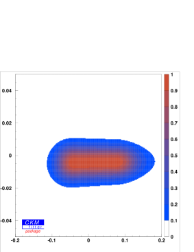
$r_{0}\,\cos\phi_{0}$

$r_{1}\,\sin\phi_{1}$

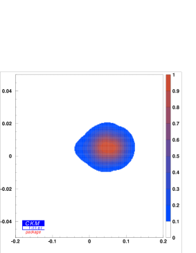
$r_{1}\,\cos\phi_{1}$

Figure 1: The result for $r_{0}\,e^{i\phi_{0}}$ and $r_{1}\,e^{i\phi_{1}}$ from the fit to $J/\psi K$ observables, see text.

The fitted parameters have reasonable orders of magnitude, although generally $r_{1}\ll r_{0}$ is expected. Notice that the preferred values for the strong phases turn out to be small. Notice furthermore that, depending on the actual size of these suppression factors, the result for $r_{0}$ and $r_{1}$ may also be interpreted as due to unexpectedly large effects from subleading SM operators.

4 $\mathbf{B\to\boldsymbol{\phi}K}$

The similar analysis for this penguin-dominated decay results in a power-counting $A_{\rm NP}(\Delta I=0)/(\mathcal{A}_{0})\lesssim\mathcal{O}(1)\,,A_{\rm NP}(\Delta I=1)/(\mathcal{A}_{0})\lesssim\mathcal{O}(\lambda)\,.$ SM estimates usually give small subleading contributions [12, 13, 14, 15]. The parametrization is completely analogous to the one of $B\to J/\psi K$. Again, tensions with the naive SM expectations are found [9]. Again only the results including isospin breaking contributions are shown. Note that since the publication of [1], the data of the time-dependent CP asymmetries changed significantly. The corresponding fit yields the $1\sigma$-ranges $r_{0}\,\cos\phi_{0}=\left[\phantom{-}0.03,\,0.48\right]$, $r_{0}\,\sin\phi_{0}=\left[-0.11,\,-0.03\right]$ , $r_{1}\,\cos\phi_{1}=\left[-0.35,\,0.10\right]$ and $r_{1}\,\sin\phi_{1}=\left[-0.09,\,-0.01\right]\,,$ favouring larger values than in $B\to J/\psi K$. Also in this case small phases are preferred. In addition, the fit yields non-vanishing values for both contributions, with the contribution to $\Delta I=0$ tending to be larger. Importantly, also here an operator with the structure $(\bar{s}b)(\bar{u}u/\bar{d}d)$ is needed to explain all deviations, and the relative size of the effects in $B\to J/\psi K$ and $B\to\phi K$ corresponds to naive expectations, when assigning the deviations to the same source.

5 $\mathbf{B\to\boldsymbol{\pi}K}$

$B\to\pi K$ decays are also penguin dominated, due to the Cabbibo suppression of their tree contributions. In addition, they are sensitive to electroweak penguin contributions. In the following, the parametrization from [16, 17] is used for the decay amplitudes. The experimental data is given in table 1. Without any assumptions on strong interaction dynamics, in the isospin limit one is left with 11 independent hadronic parameters for 9 observables. In order to test the SM against possible NP effects in these decays, one needs therefore additional dynamical input, implying a stronger model dependence. The following assumptions are used here: The tiny doubly Cabbibo suppressed penguin contribution ($\epsilon_{a}$) is set to zero, and the values from [17] for $q,q_{C}$ and the corresponding phases are used. Tensions in the fit, or incompatible values for the parameters $\epsilon_{T,3/2}$ and $\phi_{T,3/2}$ then may be taken as indication for possible NP contributions.

Observable	HFAG [9]	SM fit	NP $(I=0,1)$
$\overline{{\rm BR}}(\pi^{0}K^{-})\cdot 10^{6}$	$12.9\pm 0.6$	$12.4$	$12.8$
$\overline{{\rm BR}}(\pi^{-}\bar{K}^{0})\cdot 10^{6}$	$23.1\pm 1.0$	$23.7$	$23.3$
$\overline{{\rm BR}}(\pi^{+}K^{-})\cdot 10^{6}$	$19.4\pm 0.6$	$19.7$	$19.5$
$\overline{{\rm BR}}(\pi^{0}\bar{K}^{0})\cdot 10^{6}$	$\phantom{1}9.8\pm 0.6$	$\phantom{1}9.3$	$\phantom{1}9.7$
$\mathcal{A}_{\rm CP}(\pi^{-}\bar{K}^{0})$	$\phantom{-}0.009\pm 0.025$	$0^{*}$	$0^{*}$
$\mathcal{A}_{\rm CP}(\pi^{0}K^{-})$	$\phantom{-}0.050\pm 0.025$	$\phantom{-}0.043$	$\phantom{-}0.047$
$\mathcal{A}_{\rm CP}(\pi^{+}K^{-})$	$-0.098^{+0.012}_{-0.011}$	$-0.098$	$-0.092$
$\eta_{\rm CP}\,S_{\pi^{0}K_{S}}$	$-0.57\pm 0.17$	$-0.62$	$-0.78$
$C_{\pi^{0}K_{S}}$	$\phantom{-}0.01\pm 0.10$	$\phantom{-}0.14$	$\phantom{-}0.10$

Table 1: Experimental data for $B\to\pi K$ decays vs. various best fit results, see also text. $\chi^{2}_{\rm SM}/{\rm d.o.f.}=3.8/3$ and $\chi^{2}_{\rm\pi-\gamma}/{\rm d.o.f.}=2.6/3$.

The best fit values are shown in in table 1, showing clearly the reduction of $B\to\pi K$ puzzle for the new data. Especially the key parameter $\Delta\epsilon$ now corresponds to $|\Delta\epsilon/\epsilon_{T}|=|C/T|\in[0.22,1.00](1\sigma)\,,$ which does not seem unreasonable. This led the authors of [18] to the conclusion that the data are now compatible with the SM. On the other hand, in another paper [19] it has been concluded that the pattern of the measured time-dependent CP asymmetries shows a tension with the values predicted from $B^{-}\to\pi^{-}\pi^{0}$ with aid of $SU(3)$ arguments (fixing mainly $\epsilon_{3/2}$), leading to $S_{\pi^{0}K_{S}}\sim 1$ and $C_{\pi^{0}K_{S}}=\Delta A$, and hinting towards a electroweak penguin sector with a large weak phase. In [20] an analysis along similar lines was performed, pointing out that (i) $C_{\pi^{0}K_{S}}\simeq\Delta A$ is an approximate result of a model-independent sumrule [21], holding at the percent level, and (ii) that $S_{\pi^{0}K_{S}}\sim 1$ is extremely sensitive to ${\rm BR}(B\to\pi^{0}K^{0})$. Finally, the authors of [22] find a reduced puzzle, using the Neubert-Rosner relation for $q$ and its counterpart for colour-suppressed penguins. They find the tension not significantly relaxed by introducing modified electroweak penguins. This model-dependence clearly has to be clarified before any reliable conclusions are possible. The value for $\Delta A$ still implies large non-factorizable contributions, when interpreted in SM terms. In addition, the possible effects in $B\to J/\psi K$ and $B\to\phi K$ data should have an even more pronounced effect in $B\to\pi K$. This motivates the inclusion of NP operators along similar lines as in $B\to J/\psi K$ and $B\to\phi K$, despite the unclear situation in the SM:

The fit becomes more complicated than in the previous cases, because NP contributions with $\Delta I=1$ induce two new isospin amplitudes, corresponding to final $|K\pi\rangle$ states with $I=1/2$ or $I=3/2$. Note that in this case, the contributions with $\Delta I=1$ are not expected to be suppressed. In order to reduce the number of free parameters in the fit, and to avoid unphysical solutions, the following additional assumptions/approximations are applied: Following the experimental observation, the direct CP asymmetry in the decay $B^{-}\to\pi^{-}\bar{K}^{0}$ is forced to vanish identically, which yields the relation $r_{0}\,e^{i\phi_{0}}=-r_{1}^{(1/2)}\,\,e^{i\phi_{1}^{(1/2)}}-r_{1}^{(3/2)}\,e^{i\phi_{1}^{(3/2)}}\,.$ This effectively implies dealing with a $b\to s\bar{u}u$ operator which does not contribute to $B^{-}\to\pi^{-}\bar{K}^{0}$ in the naive factorization approximation. The amplitude parameters $\epsilon_{T,3/2}$ and $\phi_{T,3/2}$ are chosen to be equal and lie within the QCDF ranges, see [1]. For $\theta_{W}=\pi-\gamma$, the fit results in $r_{1}^{(1/2)}\in[0.02,\,0.08]$, $\phi_{1}^{(1/2)}\in[-2.84,\,-0.52]$, $r_{1}^{(3/2)}\in[0.00,\,0.23]$, and $\phi_{1}^{(3/2)}$ unconstrained, see also Table 1. However, the QCDF input breaks reparametrization invariance, therefore the fit depends on $\theta_{W}$ in an essential way, see [1, 11]. Notably, also in this scenario the measured values for the time-dependent CP asymmetry in $B\to\pi^{0}K_{S}$ are difficult to accomodate, as can be seen in table 1. With a phase differing strongly from the SM one that is possible (for example with $\theta_{W}\sim\pi/3$), however only with rather large NP contributions. While this is a first hint on a genuine NP phase, it is paid by the model-dependence mentioned before.

6 Conclusions

The work presented here pursues a model-independent approach. Assuming the dominance of an individual NP operator, the analysis of $B\to J/\psi K$, $B\to\phi K$ and $B\to K\pi$ observables allows for infering semi-quantitative information about the relative size of NP contributions to $b\to s\bar{q}q$ operators. The main conclusions to be drawn are: (i) All three modes discussed above prefer the inclusion of an operator transforming non-trivial under isospin, namely an operator with the structure $\mathcal{O}_{\rm NP}\sim(\bar{s}b)(\bar{u}u)$ provides a solution for all observed tensions. (ii) From the comparison of isospin-averaged $B\to J/\psi K$ and $B\to\phi K$ observables it is found that — after correcting for relative penguin, phase-space and normalization factors — NP contributions to $b\to s(c\bar{c}/\bar{s}s)$ operators may be of similar size (order 10% relative to a SM tree operator). (iii) In all cases, in order to explain the tensions with SM expectations for CP asymmetries without fine-tuning of hadronic parameters, one has to require non-trivial weak phases ($\theta_{W}\neq 0,\pi$), which could be due to NP, albeit the case $\theta_{W}=\pi-\gamma_{\rm SM}$ is always allowed, too. A different weak phase is only preferred in $B\to\pi K$, which is however only a very weak indication of a genuine NP phase. Consequently, these findings are still compatible with a SM scenario where non-factorizable QCD dynamics in matrix elements of subleading operators is unexpectedly large.

In the future, an improvement of experimental accuracy, in particular on the isospin-violating observables like the rate asymmetry, could lead to even more interesting constraints on the relative importance of different $b\to sq\bar{q}$ operators and their interpretation within particular NP models.

References

- [1] T. Feldmann, M. Jung, T. Mannel. JHEP 08, 066 (2008).
- [2] J. Charles, et al. Eur. Phys. J. C41, 1 (2005). Updated results and plots available at: http://ckmfitter.in2p3.fr.
- [3] R. Fleischer, T. Mannel. Phys. Lett. B506, 311 (2001).
- [4] H. Boos, T. Mannel, J. Reuter. Phys. Rev. D70, 036006 (2004).
- [5] H.-n. Li, S. Mishima. JHEP 03, 009 (2007).
- [6] M. Gronau, J. L. Rosner. Phys. Lett. B672, 349 (2009).
- [7] M. Ciuchini, M. Pierini, L. Silvestrini. Phys. Rev. Lett. 95, 221804 (2005).
- [8] S. Faller, M. Jung, R. Fleischer, T. Mannel. Phys. Rev. D79, 014030 (2009).
- [9] E. Barberio, et al. arXiv: 0808.1297 (hep–ex) (2008). Online update available at http://www.slac.stanford.edu/xorg/hfag.
- [10] M. Gronau, et al. Phys. Rev. D52, 6356 (1995).
- [11] M. Jung. Ph.D. thesis, Universität Siegen (2009). Http://dokumentix.ub.uni-siegen.de/opus/volltexte/2009/392/.
- [12] Y. Grossman, Z. Ligeti, Y. Nir, H. Quinn. Phys. Rev. D68, 015004 (2003).
- [13] A. R. Williamson, J. Zupan. Phys. Rev. D74, 014003 (2006).
- [14] H.-Y. Cheng, C.-K. Chua, A. Soni. Phys. Rev. D72, 014006 (2005).
- [15] M. Beneke. Phys. Lett. B620, 143 (2005).
- [16] M. Neubert. JHEP 02, 014 (1999).
- [17] M. Beneke, et al. Nucl. Phys. B591, 313 (2000).
- [18] M. Ciuchini, et al. Phys. Lett. B674, 197 (2009).
- [19] R. Fleischer, et al. Phys. Rev. D78, 111501 (2008).
- [20] M. Gronau, J. L. Rosner. Phys. Lett. B666, 467 (2008).
- [21] M. Gronau. Phys. Lett. B627, 82 (2005).
- [22] S. Baek, C.-W. Chiang, D. London. arXiv 0903.3086 (hep–ph) (2009).