The spatial distribution of stars
in open clusters

Abstract

In this work we study the internal spatial structure of 16 open clusters in the Milky Way spanning a wide range of ages. For this, we use the minimum spanning tree method (the $Q$ parameter, which enables one to classify the star distribution as either radially or fractally clustered), King profile fitting, and the correlation dimension ($D_{c}$) for those clusters with fractal patterns. On average, clusters with fractal-like structure are younger than those exhibiting radial star density profiles. There is a significant correlation between $Q$ and the cluster age measured in crossing time units. For fractal clusters there is a significant correlation between the fractal dimension and age. These results support the idea that stars in new-born clusters likely follow the fractal patterns of their parent molecular clouds, and eventually evolve toward more centrally concentrated structures. However, there can exist stellar clusters as old as $\sim 100$ Myr that have not totally destroyed their fractal structure. Finally, we have found the intriguing result that the lowest fractal dimensions obtained for the open clusters seem to be considerably smaller than the average value measured in galactic molecular cloud complexes.

1 Introduction

The hierarchical structure observed in some open clusters is presumably a consequence of its formation in a turbulent medium with an underlying fractal structure ([Elmegreen & Scalo (2004), Elmegreen & Scalo 2004]). Otherwise, open clusters having central star concentrations with radial star density profiles likely reflect the dominant role of gravity, either on the primordial gas structure or as a result of a rapid evolution from a more structured state ([Lada & Lada (2003), Lada & Lada 2003]). Therefore, the analysis of the distribution of stars may yield information on the formation process and early evolution of open clusters. It is necessary, however, that this kind of analysis is done by measuring the cluster structure in an objective, quantitative, as well as systematic way. Here we study the internal spatial structure in a sample of 16 open clusters spanning a wide range of ages.

2 Procedure

1. We first used VizieR ([Ochsenbein et al. (2000), Ochsenbein et al. 2000]) to search for catalogs containing both positions and proper motions of stars in open cluster regions.

2. We applied a robust non-parametric method to assign cluster memberships ([Cabrera-Caño & Alfaro (1990), Cabrera-Caño & Alfaro 1990]). This method makes no a priori assumptions about cluster and field star distributions.

3. We fitted [King (1962), King (1962)] profiles to the radial density distribution of cluster members. From these fits we obtained both the core radius ($R_{c}$) and the tidal radius ($R_{t}$).

4. Then, we used the minimum spanning tree technique (see Fig. 1) to calculate the dimensionless parameter $Q$ (see details in [Cartwright & Whitworth (2004), Cartwright & Whitworth 2004] and [Schmeja & Klessen (2006), Schmeja & Klessen 2006]). The value $Q\simeq 0.8$ separates radial clustering ($Q>0.8$) from fractal type clustering ($Q<0.8$).

   

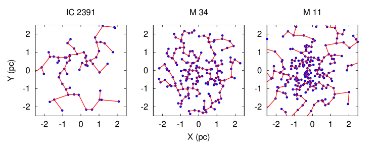
   Figure 1: The minimum spanning tree is the set of straight lines connecting the points such that the sum of their lengths is a minimum. Here we show minimum spanning trees for three open clusters, from which we can calculate the structure parameter $Q$. Star positions are indicated with blue circles and red lines represent the tree. The value of $Q$ quantifies the spatial distribution of stars. For IC 2391 the stars are distributed following an irregular fractal pattern ($Q=0.77<0.8$), for M 34 the stars are distributed roughly homogeneously ($Q=0.8$), and for M 11 the stars follow a radial density profile ($Q=1.02>0.8$).

5. Finally, we calculated the correlation dimension ($D_{c}$) and its associated uncertainty by using an algorithm which gives reliable results ([Sánchez et al. (2007), Sánchez et al. 2007a], [Sánchez & Alfaro (2008), Sánchez & Alfaro 2008]).

3 Main results

Table 1 summarizes the relevant data (ages and distances were taken from the Webda database).

Table 1: Properties of the clusters in the sample.

Name	$\log\ T$	$D$	$N_{s}$	$R_{c}$	$R_{t}$	$Q$	$D_{c}$
IC 2391	7.661	175	62	1.46	2.65	0.77	$1.74\pm 0.20$
M 11	8.302	1877	289	1.98	4.49	1.02	…
M 34	8.249	499	181	0.11	1.73	0.80	$2.04\pm 0.05$
M 67	9.409	908	354	2.21	5.92	0.98	…
NGC 188	9.632	2047	1459	2.90	10.57	0.91	…
NGC 581	7.336	2194	526	1.38	11.86	0.76	$1.79\pm 0.06$
NGC 1513	8.110	1320	156	1.55	7.73	0.72	$1.82\pm 0.09$
NGC 1647	8.158	540	683	1.23	8.86	0.70	$1.94\pm 0.02$
NGC 1817	8.612	1972	277	3.39	11.97	0.79	$1.94\pm 0.04$
NGC 1960	7.468	1318	311	2.96	8.77	0.87	…
NGC 2194	8.515	3781	228	3.17	10.31	0.85	…
NGC 2548	8.557	769	168	2.61	9.16	0.90	…
NGC 4103	7.393	1632	799	0.72	10.74	0.78	$1.85\pm 0.04$
NGC 4755	7.216	1976	196	1.11	3.50	0.94	…
NGC 5281	7.146	1108	80	0.62	2.44	0.84	…
NGC 6530	6.867	1330	145	1.43	7.47	0.67	$1.74\pm 0.09$

Note: $T$ = cluster age (Myr); $D$ = distance (pc); $N_{s}$ = number of members; $R_{c}$ = core radius (pc); $R_{t}$ = tidal radius (pc); $Q$ = structure parameter; $D_{c}$ = correlation dimension.

On average, stars in young clusters tend to be distributed following clustered, fractal-like patterns ($Q<0.8$), whereas older clusters tend to exhibit radial star density profiles ($Q>0.8$). However, the statistical analysis indicates that there is no significant correlation between $Q$ and $\log(T)$. If instead we consider the variable $T/R_{t}$, which is proportional to the cluster age measured in crossing time units (assuming nearly the same typical velocity dispersion for the open clusters), then a significant correlation is observed (Fig. 3). Additionally, we observe significant correlations (confidence levels above 96 %) between $D_{c}$ and $T$ (cluster age) and also between $D_{c}$ and $T/R_{t}$ (age in crossing time units) for those clusters with internal substructure (Fig. 3).

4 Discussion

Our results support the idea that stars in new-born cluster likely follow the fractal patterns of their parent molecular clouds, and that eventually evolve toward more centrally concentrated structures (see [Schmeja & Klessen (2006), Schemja & Klessen 2006]; [Schmeja et al. (2008), Schmeja et al. 2008], [Schmeja et al. (2009), 2009]; [Sánchez et al. (2007), Sánchez et al. 2007a], [Sánchez & Alfaro (2009), 2009]). However, this seems to be only an overall trend. The very young cluster $\sigma$ Orionis (age $\sim 3$ Myr) exhibits a radial density gradient with $Q\simeq 0.88$ ([Caballero (2008), Caballero 2008]). On the other hand, Table 1 shows open clusters as old as $\sim 100$ Myr that have not totally destroyed their clumpy structure (for example, both NGC 1513 and NGC 1647 have $Q\sim 0.7$). [Goodwin & Whitworth (2004), Goodwin & Whitworth (2004)] simulated the dynamical evolution of young clusters and showed that the survival of the initial substructure depends strongly on the initial velocity dispersion. Fractal clusters with a low velocity dispersion tend to erase their substructure rather quickly. However, if the velocity dispersion is high, such that the cluster remains supported against its own gravity or even expands, then significant levels of substructure can survive for several crossing times. Thus, our results give some observational support to [Goodwin & Whitworth (2004), Goodwin & Whitworth’s (2004)] simulations.

From Fig. 3, we can see that clusters with the smallest correlation dimensions ($D_{c}=1.74$) would have three-dimensional fractal dimensions around $D_{f}\sim 2.0$ (estimated from previous papers, see e.g. Fig. 1 in [Sánchez & Alfaro (2008), Sánchez & Alfaro 2008]). This is a very interesting result because this value is considerably smaller than the average value estimated for galactic molecular clouds in recent studies, which is $D_{f}\simeq 2.6-2.7$ ([Sánchez et al. (2005), Sánchez et al. 2005], [Sánchez et al. (2007), Sánchez et al. 2007b]). Young, new-born stars probably will reflect the conditions of the interstellar medium from which they were formed. Therefore, a group of stars born from the same cloud, i.e. born at almost the same place and time, should have a fractal dimension similar to that of the parent cloud. If the fractal dimension of the interstellar medium has a nearly universal value around 2.6-2.7, then how can some clusters exhibit such small fractal dimension values? Perhaps some clusters may develop some kind of substructure starting from an initially more homogeneous state. This possibility has been confirmed in numerical simulations ([Goodwin & Whitworth (2004), Goodwin & Whitworth 2004]), although some coherence in the initial velocity dispersion is required. Another explanation is that this difference is a consequence of a more clustered distribution of the densest gas from which stars form at the smallest spatial scales in the molecular cloud complexes, according to a multifractal scenario ([Chappell & Scalo (2001), Chappell & Scalo 2001]). Maybe the star formation process itself modifies in some (unknown) way the underlying geometry generating distributions of stars that can be very different from the distribution of gas in the parental clouds. Finally, one possibility is that the fractal dimension of the interstellar medium in the Galaxy does not have a universal value and therefore some regions form stars distributed following more clustered patterns. There is no a priori reason for assuming that $D_{f}$ has nearly the same value everywhere in the Galaxy independently of either the dominant physical processes or environmental variables. Recent simulations of supersonic isothermal turbulence done by [Federrath et al. (2009), Federrath et al. (2009)] showed that compressive forcing yields fractal dimension values for the interstellar medium significantly smaller ($D_{f}\sim 2.3$) compared to solenoidal forcing ($D_{f}\sim 2.6$). Thus, $D_{f}$ could be very different from region to region in the Galaxy depending on the main physical processes driving the turbulence. At least at galactic scales, it has been shown that there are significant differences in the fractal dimension of the distribution of star forming sites among the galaxies, contrary to the universal picture previously claimed in the literature ([Sánchez & Alfaro (2008), see Sánchez & Alfaro 2008]). So that the possibility of a non-universal fractal dimension for the interstellar medium in the Galaxy cannot, in principle, be ruled out.

Figure 2: Structure parameter $Q$ as a function of the logarithm of age divided by the tidal radius, which is nearly proportional to age in crossing times units. The dashed line at $Q=0.8$ roughly separates radial from fractal clustering. The best linear fit (equation at the top) is represented by a solid line.

Figure 3: Calculated correlation dimension as a function of age (in crossing time units). The best linear fit (equation at the top) is represented by a solid line. As reference, horizontal dashed lines indicate the values corresponding to three-dimensional distributions with fractal dimensions of $D_{f}=2.0$ and $2.5$.

References

- [Caballero (2008)] Caballero, J.A. 2008, MNRAS, 383, 375
- [Cabrera-Caño & Alfaro (1990)] Cabrera-Caño, J., & Alfaro, E.J. 1990, A&A, 235, 94
- [Cartwright & Whitworth (2004)] Cartwright, A., & Whitworth, A.P. 2004, MNRAS, 348, 589
- [Chappell & Scalo (2001)] Chappell, D., & Scalo, J. 2001, ApJ, 551, 712
- [Elmegreen & Scalo (2004)] Elmegreen, B.G., & Scalo, J. 2004, ARAA, 42, 211
- [Federrath et al. (2009)] Federrath, C., Klessen, R.S., & Schmidt, W. 2009, ApJ, 692, 364
- [Goodwin & Whitworth (2004)] Goodwin, S.P., & Whitworth, A.P. 2004, A&A, 413, 929
- [King (1962)] King, I. 1962, AJ, 67, 471
- [Lada & Lada (2003)] Lada, C.J., & Lada, E.A. 2003, ARAA, 41, 57
- [Ochsenbein et al. (2000)] Ochsenbein, F., Bauer, P., & Marcout, J. 2000, A&AS, 143, 221
- [Sánchez et al. (2005)] Sánchez, N., Alfaro, E.J., & Pérez, E. 2005, ApJ, 625, 849
- [Sánchez et al. (2007)] Sánchez, N., Alfaro, E.J., Elias, F., Delgado, A.J., & Cabrera-Caño, J. 2007a, ApJ, 667, 213
- [Sánchez et al. (2007)] Sánchez, N., Alfaro, E.J., & Pérez, E. 2007b, ApJ, 656, 222
- [Sánchez & Alfaro (2008)] Sánchez, N., & Alfaro, E.J. 2008, ApJS, 178, 1
- [Sánchez & Alfaro (2009)] Sánchez, N., & Alfaro, E.J. 2009, ApJ, 696, 2086
- [Schmeja & Klessen (2006)] Schmeja, S., & Klessen, R.S. 2006, A&A, 449, 151
- [Schmeja et al. (2008)] Schmeja, S., Kumar, M.S.N., & Ferreira, B. 2008, MNRAS, 389, 1209
- [Schmeja et al. (2009)] Schmeja, S., Gouliermis, D.A., & Klessen, R.S. 2009, ApJ, 694, 367