Fast domain wall propagation under an optimal field pulse in magnetic nanowires

Abstract

We investigate field-driven domain wall (DW) propagation in magnetic nanowires in the framework of the Landau-Lifshitz-Gilbert equation. We propose a new strategy to speed up the DW motion in a uniaxial magnetic nanowire by using an optimal space-dependent field pulse synchronized with the DW propagation. Depending on the damping parameter, the DW velocity can be increased by about two orders of magnitude compared to the standard case of a static uniform field. Moreover, under the optimal field pulse, the change in total magnetic energy in the nanowire is proportional to the DW velocity, implying that rapid energy release is essential for fast DW propagation.

Recently the study of domain wall (DW) motion in magnetic nanowires has attracted a great deal of attention, inspired both by fundamental interest in nanomagnetism as well as potential industrial applications. Many interesting applications like memory bitsCowburn ; Parkin or magnetic logic devicesAllwood involve fast manipulation of DW structures, i.e. a large magnetization reversal speed.

In general, the motion of a DW can be driven by a magnetic field Ono ; Atkinson ; Beach and/or a spin-polarized currentKlaui ; Hayashi ; Zhang ; Tatara ; Thiaville . Although the DW dynamics in systems of higher spatial dimension can be very complicated, some simple but important results were obtained by Schryer and Walker for effectively one-dimensional (1D) situationsWalker : At low field (or current density), the DW velocity $v$ is linear in the field strength $H$ until $H$ reaches a so-called Walker breakdown field $H_{w}$Walker . Within this linear regime, DW propagates as a rigid object. For $H>H_{w}$, the DW loses its rigidity and develops a complex time-dependent internal structure. The velocity can even oscillate with time due to the “breathing” of the DW width. The time-averaged velocity $\bar{v}$ decreases with the increase of $H$, resulting in a negative differential mobility. $\bar{v}$ can be again linear with $H$ approximately when $H\gg H_{w}$. The predicted $v$-$H$ characteristic is in a good agreement with experimental results on permalloy nanowiresOno ; Atkinson ; Beach . Recently a general definition of the DW velocity proper for any types of DW dynamics has been also introducedWang .

For a single-domain magnetic nanoparticle (called Stoner particle), an appropriate time-dependent but spatially homogeneous field pulse can substantially lower the switching field and increase the reversal speed since it acts as an energy source enabling to overcome the energy barrier for switching the spatially constant magnetizationSun ; Wang1 . In the present letter, we investigate the dynamics of a DW in a magnetic nanowire under a field pulse depending both on time and space. As a result, such a pulse, synchronized with the DW propagation, can dramatically increase the DW velocity by typically two orders compared with the situation of a constant field. Moreover, the total magnetic energy typically decreases with a rate being proportional to the DW velocity, i.e. the external field source can even absorb energy from the nanowire.

Figure 1: A schematic diagram of two dynamically equivalent 1D magnetic nanowire structures. (A) Easy axis is along the wire axis (z-axis); (B) Easy axis (z-axis) $\perp$ the wire axis (x-axis). The region between two dashed lines denotes the DW region.

A magnetic nanowire can be described as an effectively 1D continuum of magnetic moments along the wire axis direction. Magnetic domains are formed due to the competition between the anisotropic magnetic energy and the exchange interaction among adjacent magnetic moments. Let us first concentrate on the case of a uniaxial magnetic anisotropy: Two dynamically equivalent configurations of 1D uniaxial magnetic nanowires are schematically shown in Fig. 1. Type A shows the wire axis to be also the easy-axis (z-axis). Type B shows the easy axis (z-axis) is perpendicular to the wire axis (x-axis). Although our results described below apply to both configurations, we will focus in the following on type B. The spatio-temporal dynamics of the magnetization density $\vec{M}(x,t)$ is governed by the Landau-Lifshitz-Gilbert (LLG) equationllg

$$\frac{\partial\vec{M}}{\partial t}=-|\gamma|\vec{M}\times\vec{H}_{t}+\frac{\alpha}{M_{s}}\left(\vec{M}\times\frac{\partial\vec{M}}{\partial t}\right),$$ (1)

where $|\gamma|=2.21\times 10^{5}(rad/s)/(A/m)$ the gyromagnetic ratio, $\alpha$ the Gilbert damping coefficient, and $M_{s}$ is the saturation magnetization density. The total effective field $\vec{H}_{t}$ is given by the variational derivative of the total energy with respect to magnetization, $\vec{H}_{t}=-(\delta E/\delta\vec{M})/\mu_{0}$, where $\mu_{0}$ the vacuum permeability. The total energy $E=\int_{-\infty}^{\infty}dx\varepsilon(x)$ can be written as an integral over an energy density (per unit section-area),

$$\varepsilon(x)=-KM_{z}^{2}+J\left[\left(\frac{\partial\theta}{\partial x}\right)^{2}+\sin^{2}\theta\left(\frac{\partial\phi}{\partial x}\right)^{2}\right]-\mu_{0}\vec{M}\cdot\vec{H},$$ (2)

where $x$ is the spatial variable in the wire direction. Here $K$, $J$ are the coefficients of energetic anisotropy and exchange interaction, respectively, and $\vec{H}$ is the external magnetic field. Moreover, we have adopted the usual spherical coordinates, $\vec{M}(x,t)=M_{s}(\sin\theta\cos\phi,\sin\theta\sin\phi,\cos\theta)$ where the polar angle $\theta(x,t)$ and the azimuthal angle $\phi(x,t)$ depend on position and time.

Hence, the total field $\vec{H}_{t}$ consists of three parts: the external field $\vec{H}$, the intrinsic uniaxial field along the easy axis $\vec{H}^{K}=(2KM_{z}/\mu_{0})\hat{z}$, and the exchange field $\vec{H}^{J}$ which reads in spherical coordinates asWalker ; Hickey ,

$$H^{J}_{\theta} =\frac{2J}{\mu_{0}M_{s}}\frac{\partial^{2}\theta}{\partial x^{2}}-\frac{J\sin 2\theta}{\mu_{0}M_{s}}\left(\frac{\partial\phi}{\partial x}\right)^{2},$$

$$H^{J}_{\phi} =\frac{2J}{\mu_{0}M_{s}\sin\theta}\frac{\partial}{\partial x}\left(\sin^{2}\theta\frac{\partial\phi}{\partial x}\right).$$ (3)

Following Ref. Walker , let us focus on DW structures fulfilling $\partial\phi/\partial x=0$, i.e. all the magnetic moments rotate around the easy axis synchronously. Then the dynamical equations take the form

$$\Gamma \dot{\theta}=\alpha\left(H_{\theta}-\frac{KM_{s}}{\mu_{0}}\sin 2\theta+\frac{2J}{\mu_{0}M_{s}}\frac{\partial^{2}\theta}{\partial x^{2}}\right)+H_{\phi},$$

$$\Gamma \sin\theta\dot{\phi}=\alpha H_{\phi}-H_{\theta}+\frac{KM_{s}}{\mu_{0}}\sin 2\theta-\frac{2J}{\mu_{0}M_{s}}\frac{\partial^{2}\theta}{\partial x^{2}},$$ (4)

where we have defined $\Gamma\equiv(1+\alpha^{2})|\gamma|^{-1}$, and $H_{i}(i=r,\theta,\phi)$ are the three components of the external field in spherical coordinates. In the absence of an external field, an exact solution for a static DW is given by $\tan{\frac{\theta(x)}{2}}=\exp(x/\Delta)$ where $\Delta=\sqrt{J/(KM_{s}^{2})}$ is the width of the DW. We note that a static DW can exist in a constant field only if the field component along the easy axis is zero, $H_{z}=0$. In fact, according to Eqs. (4) static solutions need to fulfill $H_{\phi}=0$ [implying $\phi=\tan^{-1}(H_{y}/H_{x})$ is spatially constant] and

$$\frac{2J}{\mu_{0}M_{s}}\frac{\partial^{2}\theta}{\partial x^{2}}-\frac{KM_{s}}{\mu_{0}}\sin 2\theta+H_{\theta}=0$$ (5)

or, upon integration,

$$\frac{J}{\mu_{0}M_{s}}\left(\frac{\partial\theta}{\partial x}\right)^{2}+\frac{KM_{s}}{2\mu_{0}}\cos 2\theta+H_{r}(\theta)={\rm constant}.$$ (6)

Considering the two boundaries at $\theta=0(x\rightarrow-\infty)$ and $\theta=\pi(x\rightarrow+\infty)$ for the DW, we conclude $H_{r}(0)=H_{r}(\pi)$, which requires $H_{z}=0$. In this case, the stationary DW solutions under a transverse field are described as $x=\int[\sqrt{(KM_{s}^{2}\sin^{2}\theta-\mu_{0}M_{s}H\sin\theta)/J}]^{-1}d\theta$.

Thus, when an external field with a component along the easy axis is applied to the nanowire, the DW is expected to move. We use a travelling-wave ansatz to describe rigid DW motionWalker ,

$$\tan\frac{\theta(x,t)}{2}=\exp\left(\frac{x-vt}{\Delta}\right),$$ (7)

where the DW velocity $v$ is assumed to be constant. Substituting this trial function into Eq. (4), the dynamic equations become

$$\Gamma\sin\theta v=-\Delta(\alpha H_{\theta}+H_{\phi}),\quad\Gamma\sin\theta\dot{\phi}=\alpha H_{\phi}-H_{\theta}.$$ (8)

Eq. (8) describes the dependence of the linear velocity $v$ and the angular velocity $\dot{\phi}$ on the external field $\vec{H}$. Our following results discussion will be based on Eqs. (8).

Let us first turn to the case of a static field case applied along the easy axis (z-axis in type B of Fig. 1), $H_{\theta}=-H\sin\theta,H_{\phi}=0$. Here we recover the well-known static solution for a uniaxial anisotropySlonczewski ,

$$v=\frac{|\gamma|\Delta H}{\alpha+\alpha^{-1}},$$ (9)

where the azimuthal angle $\phi(t)=\phi(0)+|\gamma|Ht/(1+\alpha^{2})$ is spatially constant (i.e. $\partial\phi/\partial x=0$) and increases linearly with time.

Let us now allow the applied external field to depend both on space and time. Our task is to design, under a fixed field magnitude $H$, an optimal field configuration $\vec{H}(x,t)$ to increase the DW velocity as much as possible. From Eqs. (8), we find a manifold of solutions of specific space-time field configurations described by a parameter $u$,

$$H_{r}(x,t)= H\cos\theta,\quad H_{\theta}(x,t)=-H\sin\theta/\sqrt{1+u^{2}},$$

$$H_{\phi}(x,t)=-uH\sin\theta/\sqrt{1+u^{2}}.$$ (10)

The velocities $v$ and $\dot{\phi}$ reads

$$v=\frac{|\gamma|\Delta H}{1+\alpha^{2}}\frac{\alpha+u}{\sqrt{1+u^{2}}},\quad\dot{\phi}=\frac{|\gamma|H}{1+\alpha^{2}}\frac{1-\alpha u}{\sqrt{1+u^{2}}}.$$ (11)

The previous static field case is recovered for $u=0$. The maximum of the velocity $v_{m}$ with regard to $u$ us reached for $u=1/\alpha$,

$$v_{m}=\frac{|\gamma|\Delta H}{\sqrt{1+\alpha^{2}}},$$ (12)

where the angular velocity is zero, $\dot{\phi}=0$. On the other hand, $\dot{\phi}$ attains a maximum for $u=-\alpha$, where, in turn, the linear velocity vanishes. In Fig. 2 we have plotted the dependence of the velocity on the parameter $u$ for different damping strengths and typical values for the DW width $\Delta$ and the magnitude $H$ of the external field.

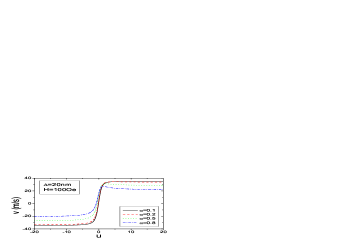
Figure 2: (Color online) The DW propagation velocity $v$ versus the parameter $u$ at the different damping values $\alpha=0.1,0.2,0.5,0.8$. The other parameters are chosen as $\Delta=20nm$ and $H=100{\rm Oe}$.

To understand the physical meaning of the maximum velocity $v_{m}$, we note that, according to Eqs. (8), the field components $H_{\theta}$ and $H_{\phi}$ are required to be proportional to $\sin\theta$ to ensure the constant velocity under the rigid DW approximation. Moreover, at $u=1/\alpha$ we have $H_{\theta}=\alpha H_{\phi}$, and from the identity

$$(\alpha H_{\theta}+H_{\phi})^{2}+(\alpha H_{\phi}-H_{\theta})^{2}=(1+\alpha^{2})(H^{2}-H_{r}^{2}),$$ (13)

we conclude that the term $(\alpha H_{\theta}+H_{\phi})$ is maximal resulting in a maximal velocity according to Eqs. (8). As a result, the new velocity under the optimal field pulse is larger by a factor of $v_{m}/v=\sqrt{1+\alpha^{2}}/\alpha\approx 1/\alpha$ compared to a constant field with the same field magnitude. To give a practical example, the typical value for the damping parameter in permalloy is $\alpha=0.01$ which results in an increase of the DW velocity by a factor of $100$.

It is instructive to also analyze the optimal field pulse according to Eq. (10) with $u=1/\alpha$ in its cartesian components,

$$H_{x}(x,t)=H\sin 2\theta(1-\alpha/\sqrt{1+\alpha^{2}})/2,$$

$$H_{y}(x,t)=-H\sin\theta/\sqrt{1+\alpha^{2}},$$ (14)

$$H_{z}(x,t)=H(\cos^{2}\theta+\alpha\sin^{2}\theta/\sqrt{1+\alpha^{2}}),$$

where $\theta$ follows the wave-like motion $\tan\frac{\theta(x,t)}{2}=\exp(\frac{x}{\Delta}-\frac{|\gamma|H}{\sqrt{1+\alpha^{2}}}t)$. In Fig. 3 we plotted these quantities at $t=0$ around the DW center where the main spatial variation of the pulse occurs. Note that the space-dependent field distribution should move with the same speed $v_{m}$ synchronized with the DW propagation. Near the DW center the components $H_{x}$ and $H_{z}$ are (almost) zero whereas a large transverse component $H_{y}$ is required to achieve fast DW propagation. Qualitatively speaking, the transverse field causes a precession of the magnetization resulting in its reversal. This finding is consistent with recent micromagnetic simulations showing that the DW velocity can be largely increased by applying an additional transverse fieldtransverse .

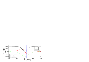
Figure 3: (Color online) The $x,y,z$ components of the optimal field pulse. The parameters are chosen as $\alpha=0.01$, $\Delta=20nm$ for permalloyBeach . The field magnitude is $H=100{\rm Oe}$.

It is also interesting to study the energy variation under the optimal field pulse,

$$\frac{dE}{dt}=-\mu_{0}\int_{-\infty}^{+\infty}dx\left(\frac{\partial\vec{M}}{\partial t}\cdot\vec{H}_{t}+\vec{M}\cdot\frac{\partial\vec{H}}{\partial t}\right)\equiv P_{\alpha}+P_{h}.$$ (15)

The first term $P_{\alpha}$ is the intrinsic damping power due to all kinds of damping mechanisms described by the phenomenological parameter $\alpha$. According to the LLG equation $P_{\alpha}=-\frac{\mu_{0}\alpha}{|\gamma|M_{s}}\int_{-\infty}^{+\infty}dx(\frac{\partial M}{\partial t})^{2}$ is always negativeSun , implying an energy loss. $P_{h}$ is the external power due to the time-dependent external field. From Eq. (11), both powers are obtained as

$$P_{\alpha}=-\frac{2\alpha}{1+\alpha^{2}}\mu_{0}|\gamma|M_{s}\Delta H^{2},$$ (16)

$$P_{h}= \frac{2\alpha(\sqrt{1+u^{2}}-1)-2u}{(1+\alpha^{2})\sqrt{1+u^{2}}}\mu_{0}|\gamma|M_{s}\Delta H^{2},$$ (17)

such that the total energy change rate is

$$\frac{dE}{dt}=-2\mu_{0}M_{s}Hv=-\frac{2(\alpha+u)\mu_{0}|\gamma|M_{s}\Delta H^{2}}{(1+\alpha^{2})\sqrt{1+u^{2}}}.$$ (18)

Note that the intrinsic damping power is independent of the parameter $u$ and always negative, whereas the total energy change rate is proportional to the negative DW velocity. Thus, for positive velocities ($u>-\alpha$) the total magnetic energy decreases while it grows for negative velocities ($u<-\alpha$). In the former case energy is absorbed by the external field source while in the latter case the field source provides energy to the system. The optimal field source helps to rapidly release or gain magnetic energy which is essential for fast DW motion. This aspect is very different from the reversal of a Stoner particle where the time-dependent field is always needed to provide energy to the system to overcome the energy barrierSun .

Moreover, our new strategy of employing space-dependent field pulses can also be applied to uniaxial anisotropies of arbitrary type: Let $w(\theta)$ be the uniaxial magnetic energy density. The static DW solution in the absence of an external field reads $x=\int\chi^{-1}(\theta)d\theta$, where

$$\chi(\theta)=\sqrt{[w(\theta)-w_{0}]/J}.$$ (19)

Here $w_{0}$ is the minimum energy density for magnetization along the easy axis. By performing analogous steps as before, we obtain the the optimal velocity as $v_{m}=\frac{|\gamma|H}{\sqrt{1+\alpha^{2}}\chi_{max}}$, where $\chi_{max}$ denotes the maximum of $\chi(\theta)$ throughout all $\theta$.

On the other hand, our approach is not straightforwardly extended to the case of a magnetic wire with biaxial anisotropy. To see this, consider, a biaxial anisotropy $\varepsilon_{i}=-KM_{z}^{2}+K^{\prime}M_{x}^{2}$ where the coefficients $K$, $K^{\prime}$ correspond to the easy and hard axis, respectivelyWalker . The LLG equations read

$$\Gamma\dot{\theta}=\alpha\left(H_{\theta}-\frac{KM_{s}}{\mu_{0}}\sin 2\theta-\frac{K^{\prime}M_{s}}{\mu_{0}}\sin 2\theta\cos^{2}\phi\right.$$

$$\left.+\frac{2J}{\mu_{0}M_{s}}\frac{\partial^{2}\theta}{\partial x^{2}}\right)+H_{\phi}+\frac{K^{\prime}M_{s}}{\mu_{0}}\sin\theta\sin 2\phi,$$

$$\Gamma\sin\theta\dot{\phi}=\alpha H_{\phi}-H_{\theta}+\frac{KM_{s}}{\mu_{0}}\sin 2\theta-\frac{2J}{\mu_{0}M_{s}}\frac{\partial^{2}\theta}{\partial x^{2}}$$

$$+\frac{K^{\prime}M_{s}}{\mu_{0}}\sin 2\theta\cos^{2}\phi+\frac{\alpha K^{\prime}M_{s}}{\mu_{0}}\sin\theta\sin 2\phi.$$ (20)

Let us assume $\phi(x,t)=\phi_{0}$ is a constant determined by the applied field. Substituting the travelling-wave ansatz $\tan\frac{\theta(x,t)}{2}=\exp\left(\frac{x-vt}{\Delta}\right)$, where now $\Delta=\sqrt{J/(K+K^{\prime}\cos^{2}\phi_{0})}/M_{s}$, into Eqs. (20) we obtain

$$\Gamma\sin\theta v=-\Delta(\alpha H_{\theta}+H_{\phi}+K^{\prime}M_{s}\sin\theta\sin 2\phi_{0}/\mu_{0}),$$ (21)

$$\alpha K^{\prime}M_{s}\sin\theta\sin 2\phi_{0}/\mu_{0}+(\alpha H_{\phi}-H_{\theta})=0.$$ (22)

For a static field along z-axis $H_{\theta}=-H\sin\theta,H_{\phi}=0$, the solution is just the Walker’s result $v=|\gamma|\Delta H/\alpha$ (Note here $\Delta$ also depends on $H$)Walker . To implement our new strategy, we need to find the maximum of the right-hand side of Eq. (21) under two constraints of Eq. (22) and Eq. (13) with $H_{\theta}$ and $H_{\phi}$ being proportional to $\sin\theta$. The unique solution to this problem is indeed a constant field along the z-axis which is thus the optimal field configuration.

In summary, our theory is general and can be applied to a magnetic nanowire with a uniaxial anisotropy which can be from shape, magneto-crystalline or the dipolar interaction. The experimental challenge of our proposal is obviously the generation of a field pulse focused on the DW region and synchronized with its motion. However, the field source synchronization velocity can be pre-calculated from the material parameters. As for the required localized field (See Fig. 3), we propose to employ a ferromagnetic scanning tunneling microscope (STM) tip to produce a localized field perpendicular to the wire axisMichlmayr and use a localized current to produce an Oersted field along the wire axisMichlmayr1 . Moreover, such required localized fields may also be produced by nano-ferromagnets with strong ferromagnetic (or antiferromagnetic) coupling to the nanowire. We also point out that, although the field source typically does not consume energy but gain energy from the magnetic nanowire, the pulse source may still require excess energy to overcome effects such as defects pinning, which is not included in our model. At last, the generalization of the strategy beyond the rigid DW approximation, and to DW motion induced by spin-polarized current will also be attractive direction of future research.

Z.Z.S. thanks the Alexander von Humboldt Foundation (Germany) for a grant. This work has been supported by Deutsche Forschugsgemeinschaft via SFB 689.

References

- (1) R. P. Cowburn, Nature (London) 448, 544 (2007).
- (2) S. S. P. Parkin, M. Hayashi, and L. Thomas, Science 320, 190 (2008).
- (3) D. A. Allwood, et al., Science 309, 1688 (2005).
- (4) T. Ono, et al., Science, 284, 468 (1999).
- (5) D. Atkinson, et al., Nature Mater. 2, 85 (2003).
- (6) G. S. D. Beach, et al., Nature Mater. 4, 741 (2005); G. S. D. Beach, et al., Phys. Rev. Lett. 97, 057203 (2006); J. Yang, et al., Phys. Rev.B 77 014413 (2008).
- (7) M. Klaui, et al., Phys. Rev. Lett. 94, 106601 (2005).
- (8) M. Hayashi, et al., Phys. Rev. Lett. 96, 197207 (2006); L. Thomas, et al., Nature (London) 443, 197 (2006); M. Hayashi, et al., Phys. Rev. Lett. 98, 037204 (2007).
- (9) S. Zhang and Z. Li, Phys. Rev. Lett. 93, 127204 (2004).
- (10) G. Tatara and H. Kohno, Phys. Rev. Lett. 92, 086601 (2004).
- (11) A. Thiaville, et al., Europhys. Lett. 69, 990 (2005).
- (12) N. L. Schryer and L. R. Walker, J. Appl. Phys. 45, 5406 (1974).
- (13) X. R. Wang, P. Yan, and J. Lu, Europhys. Lett. 86, 67001 (2009); X. R. Wang, et al., Ann. Phys. (N.Y.) 324, 1815 (2009).
- (14) Z. Z. Sun and X.R. Wang, Phys. Rev. Lett. 97, 077205 (2006); Phys. Rev. B 73, 092416 (2006); ibid. 74, 132401 (2006).; X. R. Wang and Z. Z. Sun, Phys. Rev. Lett. 98, 077201 (2007).
- (15) X. R. Wang, et al., Europhys. Lett. 84, 27008 (2008).
- (16) Z. Z. Sun and X. R. Wang, Phys. Rev. B 71, 174430 (2005), and references therein.
- (17) M. C. Hickey, Phys. Rev. B 78, 180412(R) (2008).
- (18) A. P. Malozemoff and J. C. Slonczewski, Domain Walls in Bubble Materials, (Academic, New York, 1979).
- (19) M. T. Bryan, et al., J. Appl. Phys. 103, 073906 (2008).
- (20) T. Michlmayr, et al., J. Appl. Phys. 99, 08N502 (2006).
- (21) T. Michlmayr, et al., J. Phys. D: Appl. Phys. 41, 055005 (2008).