The phase diagram of Lévy spin glasses

Abstract

We study the Lévy spin-glass model with the replica and the cavity method. In this model each spin interacts through a finite number of strong bonds and an infinite number of weak bonds. This hybrid behaviour of Lévy spin glasses becomes transparent in our solution: the local field contains a part propagating along a backbone of strong bonds and a Gaussian noise term due to weak bonds. Our method allows to determine the complete replica symmetric phase diagram, the replica symmetry breaking line and the entropy. The results are compared with simulations and previous calculations using a Gaussian ansatz for the distribution of fields.

1 Introduction

The prototype mean-field model of spin glasses is the Sherrington-Kirkpatrick (SK) model [1, 2, 3]. In this fully-connected (FC) system any pair of spins is coupled through weak interactions, of order $\mathcal{O}(N^{-1/2})$ in the total number of spins $N$, whose values are drawn independently from a Gaussian distribution.

Within the assumption that the free-energy landscape contains one single valley, the effective field on a given spin is a sum of a large number of uncorrelated random variables with a finite variance and the usual central limit theorem (CLT) holds. As a consequence, the effective field follows a Gaussian distribution fully characterized by its first two moments, leading to a description in terms of two observables: the magnetization and the Edwards-Anderson order parameter. The CLT reflects the independence of the macroscopic behavior of the system with respect to the details of the coupling distribution. The existence of a CLT in the SK model is technically very convenient and simplifies the replica and the cavity method at high temperatures $T$. At low temperatures extreme values become important and a more complicated description is necessary. The success of the cavity and replica method lies in the detailed and exact description they give of the intricate behavior of the SK model at low temperatures, characterized by the presence of several degenerate states separated by infinite barriers [3].

However, it was shown that materials composed of magnetic impurities, randomly distributed in a non-magnetic host and interacting through the RKKY dipolar potential, exhibit a Cauchy distribution of effective fields. This is in particular true for a small concentration of magnetic impurities [4, 5]. An analogous result was obtained in a spatially disordered system of particles with dipolar interactions [6]. These results suggest that the choice of a coupling distribution that allows a wider variation of coupling strengths would be more realistic than the traditional Gaussian assumption used in mean-field models for spin glasses.

Disordered systems in which the randomness of the disorder variable $J$ is modelled by a distribution $P(J)$ that has a power-law decay $P(J)\sim|J|^{-1-\alpha}$ ($\alpha<2$), for large $|J|$, have attracted less interest. A possible reason is the technical challenge to deal with distributions that do not fulfill the classical CLT. The heavy tails of $P(J)$ give rise to the divergence of the second moment of the distribution, which invalidates the application of classical CLT. In this case, the generalized CLT of Lévy and Gnedenko holds [7, 8], and the sum of a large number of independent random variables drawn from $P(J)$ follows the same distribution as the individual summands, exhibiting only different scale factors. The role of the large tails of $J$ has proven to be crucial to the long time or large size properties of different disordered systems [9]. As examples in this context, we mention the theory of random matrices [10, 11, 12], diffusion processes [13] and the portfolio optimization problem in theoretical finance [14].

A FC model of spin glasses with interactions drawn from a distribution with power-law tails (a Lévy spin glass) was introduced by Cizeau and Bouchaud [15]. In Lévy spin glasses every spin interacts with infinitely many weak bonds of order $\mathcal{O}\left(N^{-1/\alpha}\right)$ and a finite number of strong bonds of order $\mathcal{O}\left(1\right)$. In this sense the model is a hybrid between a FC spin glass, like the SK model, and a finitely connected (FiC) spin glass, like the Viana-Bray model [16]. The authors of [15] studied the model with the cavity method under the assumption that the distribution of effective fields is Gaussian. They found a spin glass phase stable under replica symmetry breaking and it was conjectured that at zero temperature the stability of replica symmetry is restored for $\alpha<1$. Recently, this model has been studied with replica theory [17]. The effective field distribution is not Gaussian. In [17] a complete phase diagram and a discussion of replica symmetry breaking was not given.

The purpose of this paper is to improve upon the foregoing studies by deriving the complete phase diagram without the Gaussian assumption, the entropy and the stability to replica symmetry breaking effects. We propose a method that consists in the insertion of a small cutoff in the distribution of the couplings $P(J)$, which gives rise to a natural distinction between “weak bonds” and “strong bonds”. This allows us to solve the problem through both the replica method and the cavity method. We obtain a solvable self-consistent equation for the distribution of effective fields. Formally this equation is similar to the self-consistent equation for the effective field distribution of a FiC spin-glass system on a random graph [18] and a straightforward implementation of the population dynamics algorithm [19] is possible. Therefore, the procedure allows us to obtain the complete phase diagram of the model for all Lévy distributions in contrast to previous works [15, 17]. We include a skewness parameter in the definition of the model, responsible for controlling the relative weight between the positive and the negative tails of the coupling distribution. The dependence of the different phases on this parameter is shown in the phase diagrams. The results are compared with simulations. We calculate the entropy of the system and the stability against replica symmetry breaking. Our results are compared with those obtained by Cizeau and Bouchaud [15].

The paper is organized as follows. In section 2, we define the model. We explain how to solve the model through replica theory in section 3 and through the cavity method in section 4. In these sections we calculate the distribution of effective fields and compare them with the Gaussian assumption on the distribution of those fields. The behavior of the magnetization is compared with simulations. In section 5 we derive the stability condition against replica symmetry breaking. The order parameter equations, derived in sections 3, 4 and 5, are solved numerically to obtain the phase diagrams and the entropy in sections 6 and 7. In section 8 we present our conclusions. The effect of the different parameters of the Lévy distributions is shown in appendix A. Some details of the replica calculations are given in appendix B.

2 The Lévy spin glass

We study a FC system of $N$ Ising spins $\sigma_{i}=\pm 1$ ($i=1,\dots,N$) with the Hamiltonian

$$H=-\sum_{i<j}J_{ij}\sigma_{i}\sigma_{j},$$ (1)

where the symmetric couplings $\{J_{ij}\}$ are i.d.d.r.v. drawn from a stable distribution $P^{J_{1},\gamma,J_{0}}_{\alpha}(J)$. We define the stable distributions $P^{J_{1},\gamma,J_{0}}_{\alpha}(J)$ through their characteristic function $L^{J_{1},\gamma,J_{0}}_{\alpha}(q)$:

$$P^{J_{1},\gamma,J_{0}}_{\alpha}(J)\equiv\int\frac{dq}{2\pi}\exp\left(-iqJ\right)L^{J_{1},\gamma,J_{0}}_{\alpha}(q).$$ (2)

The characterstic function is of the form

$$L^{J_{1},\gamma,J_{0}}_{\alpha}(q)=\exp\left[i\frac{qJ_{0}}{N}-\left|\frac{J_{1}q}{\sqrt{2}N^{1/\alpha}}\right|^{\alpha}\left(1-i\gamma\Phi{\rm sign}(q)\right)\right].$$ (3)

The distribution $P^{J_{1},\gamma,J_{0}}_{\alpha}(J)$ is characterized by four parameters: the exponent $\alpha\in(0,1)\cup(1,2]$, the skewness $\gamma\in[-1,1]$, the scale parameter $J_{1}>0$ and the shift $J_{0}\in\mathbb{R}$. The quantity $\Phi$ is given by $\Phi=\tan{(\frac{\alpha\pi}{2})}$. The scaling with $N$ in eq. (3) ensures that the Hamiltonian (1) is of order $\mathcal{O}(N)$. Lévy distributions contain two different parameters that control the bias in the couplings: $J_{0}$ and $\gamma$. We refer the reader to appendix A for a discussion of the role of $\alpha$ and $\gamma$. For $\alpha=1$ and $\gamma\neq 0$ the quantity $\Phi$ has a different expression and we will not consider this case in the sequel.

The SK model is obtained for $\alpha=2$ independent of $\gamma$: in this case the distribution $P^{J_{1},\gamma,J_{0}}_{\alpha}(J)$ is Gaussian with mean $J_{0}/N$ and variance $J_{1}^{2}/N$ [1]. For $\alpha<2$ and $-1<\gamma<1$, the asymptotic behavior $\rho(J)$ of $P^{J_{1},\gamma,J_{0}}_{\alpha}(J)$ for $|J|\rightarrow\infty$ can be derived from the explicit form of $L^{J_{1},\gamma,J_{0}}_{\alpha}(q)$:

$$\rho(J)\equiv N\lim_{|J|\rightarrow\infty}P^{J_{1},\gamma,J_{0}}_{\alpha}(J)=\left(1+\gamma{\rm sign}J\right)\frac{C_{\alpha}}{|J|^{\alpha+1}},$$ (4)

where

$$C_{\alpha}=\left(\frac{J_{1}}{\sqrt{2}}\right)^{\alpha}\frac{1}{\pi}\sin\left(\frac{\alpha\pi}{2}\right)\Gamma(\alpha+1).$$ (5)

Accordingly, the integrals for the second and higher moments of the distribution diverge for $\alpha<2$ due to the power-law decay illustrated by eq. (4).

We can define stable distributions through (3) without losing any generality, see for example [20, 21]. We remark that there are many equivalent definitions possible for the characteristic function $L$, see [21]. Loosely speaking, a random variable $x$ is stable if the sum of a given number of independent and identical copies of $x$ is characterized by the same distribution as the original variable, exhibiting only a different scale and shift.

3 The replica method

3.1 The distribution of effective fields

In order to study the thermodynamic behavior of the Lévy spin glass we employ the replica method [3]. The partition function of the system at inverse temperature $\beta=T^{-1}$ is defined by

$$Z=\sum_{\left\{\sigma\right\}_{i=1..N}}\exp{\Big{[}-\beta H\left(\left\{\sigma\right\}_{i=1..N}\right)\Big{]}},$$ (6)

with $H\left(\left\{\sigma\right\}_{i=1..N}\right)$ given by eq. (1). The averaged free-energy per spin $f$ can be written as follows

$$f=-\lim_{N\rightarrow\infty}\lim_{n\rightarrow 0}\frac{1}{\beta Nn}\ln{\overline{Z^{n}}}.$$ (7)

The symbol $\overline{(\dots)}$ denotes the average over the quenched random couplings $\{J_{ij}\}$ with the distribution $P^{J_{1},\gamma,J_{0}}_{\alpha}(J)$. The quantity $\overline{Z^{n}}$ is computed for positive integers $n$ and the limit $n\rightarrow 0$ is taken through an analytic continuation to real values.

However, the integer moments $\overline{Z^{n}}$ of the partition function diverge for real $\beta$ due to the power-law behavior of $P^{J_{1},\gamma,J_{0}}_{\alpha}(J)$ for $|J|\rightarrow\infty$. As noted in reference [17], the introduction of an imaginary temperature $\beta=-ik$, with a real parameter $k>0$, allows a straightforward calculation of the average $\overline{Z^{n}}$ by means of the definition of the characteristic function, eq. (3). However, it is not possible to write the averaged $\overline{Z^{n}}$ in terms of the two standard order-parameters usually employed in the description of FC systems, i.e., the magnetization and the spin-glass order parameter. Therefore, it is necessary to use the replica method, as developed to deal with FiC spin glasses [22]. The macroscopic behavior is characterized in terms of a non-Gaussian effective field distribution. This procedure was followed in [17]. Following their calculations we find the equation for the free energy $f$ in the limit $N\rightarrow\infty$:

$$f=f_{1}+f_{2},$$ (8)

with

$$ikf_{1} =-\lim_{n\rightarrow 0}\frac{1}{2n}\sum_{\bm{\sigma}\bm{\tau}}\Big{[}-\Big{(}\frac{J_{1}k}{\sqrt{2}}\Big{)}^{\alpha}|\bm{\sigma}.\bm{\tau}|^{\alpha}\left(1+i\gamma\rm{sign}(\bm{\sigma}\cdot\bm{\tau})\Phi\right)-ikJ_{0}(\bm{\sigma}.\bm{\tau})\Big{]}P(\bm{\sigma})P(\bm{\tau})\,\,,$$ (9)

$$ikf_{2} =\lim_{n\rightarrow 0}\frac{1}{n}\log{\biggl{\{}\sum_{\bm{\sigma}}\exp\left[-\sum_{\bm{\tau}}\Big{[}-\Big{(}\frac{J_{1}k}{\sqrt{2}}\Big{)}^{\alpha}|\bm{\sigma}.\bm{\tau}|^{\alpha}\left(1+i\gamma\rm{sign}(\bm{\sigma}\cdot\bm{\tau})\Phi\right)-ikJ_{0}(\bm{\sigma}.\bm{\tau})\Big{]}P(\bm{\tau})\right]\biggr{\}}}.$$

The order parameter $P(\bm{\sigma})$, with $\bm{\sigma}=\left(\sigma^{1},\sigma^{2},\ldots,\sigma^{n}\right)$, fulfills the self-consistent equation

$$P(\bm{\sigma}) =\frac{\exp\left(\sum_{\bm{\tau}}P(\bm{\tau})\left[-ikJ_{0}\bm{\sigma}\cdot\bm{\tau}-\left|\frac{J_{1}k\bm{\sigma}\cdot\bm{\tau}}{\sqrt{2}}\right|^{\alpha}\left(1+i\gamma\rm{sign}(\bm{\sigma}\cdot\bm{\tau})\Phi\right)\right]\right)}{\sum_{\bm{\sigma}}\exp\left(\sum_{\bm{\tau}}P(\bm{\tau})\left[-ikJ_{0}\bm{\sigma}\cdot\bm{\tau}-\left|\frac{J_{1}k\bm{\sigma}\cdot\bm{\tau}}{\sqrt{2}}\right|^{\alpha}\left(1+i\gamma\rm{sign}(\bm{\sigma}\cdot\bm{\tau})\Phi\right)\right]\right)}.$$ (11)

We make the replica-symmetric (RS) ansatz,

$$P(\bm{\sigma})=\int dhW(h)\prod^{n}_{a=1}\frac{\exp\left(-ikh\sigma^{a}\right)}{2\cosh\left(-ikh\sigma^{a}\right)},$$ (12)

which defines the field distribution $W(h)$. Substitution of (12) in (11) gives:

$$W(h)=\int\frac{ds}{2\pi}\exp{(ish)}\exp\Bigg{\{}-\int dhW(h)\int\frac{d\hat{J}dJ}{2\pi}$$

$$\times\left[\left(\frac{J_{1}}{\sqrt{2}}\right)^{\alpha}|\hat{J}|^{\alpha}\Big{(}1+i\gamma\Phi{\rm sign}(\hat{J})\Big{)}+iJ_{0}\hat{J}\right]\exp\left[i\hat{J}J\right]f(J,h,s)\Bigg{\}}.$$ (13)

The function $f(J,h,s)$ is defined as

$$f(J,h,s)\equiv\exp{\left(-\frac{is}{\beta}{\rm atanh}\Big{[}\tanh\left(\beta J\right)\tanh\left(\beta h\right)\Big{]}\right)}.$$ (14)

The analytic continuation of $T$ to real values has been achieved by taking $k=i\beta$ at the end of the calculation. Using eqs. (56)-(60) from appendix B, we integrate in eq. (13) over the $\hat{J}$ variable to obtain the following simplified expression for $W(h)$

$$0<\alpha < 1:$$

$$W(h) = \int\frac{ds}{2\pi}\exp{\Bigg{\{}ish-isJ_{0}m+\int dhW(h)\int_{-\infty}^{\infty}dJ\rho(J)\Big{[}f(J,h,s)-1\Big{]}\Bigg{\}}},$$ (15)

$$1<\alpha<2:$$

$$W(h)=\int\frac{ds}{2\pi}\exp{\Big{(}ish-isJ_{0}m\Big{)}}$$

$$\times\exp{\Bigg{\{}\int dhW(h)\int_{-\infty}^{\infty}dJ\rho(J)\Big{[}f(J,h,s)-f^{\prime}(0,h,s)J-1\Big{]}\Bigg{\}}},$$ (16)

where $f^{\prime}(0,h,s)=\frac{\partial f(J,h,s)}{\partial J}\Big{|}_{J=0}$. The distribution of couplings $\rho(J)$ is defined by eq. (4). The RS magnetization $m$ and the RS spin-glass order-parameter $q$ are determined through the averages

$$m=\int dhW(h)\tanh{(\beta h)},\qquad q=\int dhW(h)\tanh^{2}{(\beta h)}.$$ (17)

Only the large tail behavior of the distribution $P^{J_{1},\gamma J_{0}}_{\alpha}$ appears in the equations (15) and (16). This could mean that the system exhibits a certain degree of universality: the thermodynamic behavior only depends on the large tail behavior of the coupling distribution $P(J)$. The distribution $\rho(J)$ is symmetric when $\gamma=0$, with eqs. (15) and (16) reducing to a single equation, obtained previously in [17].

3.2 The normalization of the coupling distribution through a cutoff

The main difficulty in eqs. (15) and (16) concerns the normalization of $\rho(J)$ since the integral $\int dJ\rho(J)$ diverges for $\alpha<2$. Therefore, it is not possible to normalize the distribution. This invalidates the numerical calculation of $W(h)$ through the population dynamics algorithm [23] because it is not possible to sample random numbers from a non-normalizable distribution.

In this subsection we propose a simple procedure that allows to normalize $\rho(J)$ and to derive a self-consistent equation for $W(h)$ which is similar to the order-parameter equation of FiC spin glasses on random graphs. The numerical solution of this equation can be obtained through population dynamics.

The method consists of the insertion of a temperature dependent cutoff $T\epsilon>0$ in the integrals over $J$ occurring in eqs. (15) and (16), splitting each of them into an integral around zero (from $-T\epsilon$ to $T\epsilon$) plus an integral over the couplings that satisfy $|J|>T\epsilon$. Assuming $T\epsilon\ll 1$, the integrals around zero can be analytically performed by expanding $f(J,h,s)$ around $J=0$ up to order $\mathcal{O}(J^{2})$, resulting in the following equations

$$0<\alpha<1:$$

$$\int_{-\infty}^{\infty}dJ\rho(J)\Big{[}f(J,h,s)-1\Big{]}=-2is\gamma C_{\alpha}\tanh{(\beta h)}\frac{(T\epsilon)^{1-\alpha}}{1-\alpha}-s^{2}C_{\alpha}\tanh^{2}{(\beta h)}\frac{(T\epsilon)^{2-\alpha}}{2-\alpha}$$

$$+\int_{-\infty}^{\infty}dJ\rho(J)\Big{[}\Theta(J-T\epsilon)+\Theta(-J-T\epsilon)\Big{]}\Big{[}f(J,h,s)-1\Big{]},$$ (18)

$$1<\alpha<2:$$

$$\int_{-\infty}^{\infty}dJ\rho(J)\Big{[}f(J,h,s)-f^{\prime}(0,h,s)J-1\Big{]}=-s^{2}C_{\alpha}\tanh^{2}{(\beta h)}\frac{(T\epsilon)^{2-\alpha}}{2-\alpha}$$

$$\ \ \ \ \ \ \ +\int_{-\infty}^{\infty}dJ\rho(J)\Big{[}\Theta(J-T\epsilon)+\Theta(-J-T\epsilon)\Big{]}\Big{[}f(J,h,s)-f^{\prime}(0,h,s)J-1\Big{]}.$$ (19)

The symbol $\Theta(J)$ denotes the Heaviside step function: $\Theta(J)=1$ if $J>0$ and $\Theta(J)=0$ otherwise. We define the normalized distribution $P_{\epsilon}(J)$ in terms of $\rho(J)$

$$P_{\epsilon}(J)\equiv\frac{\alpha(T\epsilon)^{\alpha}}{2C_{\alpha}}\rho(J)\Big{[}\Theta(J-T\epsilon)+\Theta(-J-T\epsilon)\Big{]}.$$ (20)

Subsituting eqs. (18) and (19) in, respectively, eqs. (15) and (16) the integrals over $s$ can be analytically calculated:

$$W_{\epsilon}(h)=\sum^{\infty}_{k=0}\exp\left(-c\right)\frac{c^{k}}{k!}\int\left(\prod^{k}_{r=1}dh_{r}W_{\epsilon}(h_{r})\right)\int\left(\prod^{k}_{r=1}dJ_{r}P_{\epsilon}(J_{r})\right)\int\mathcal{D}z$$

$$\times\delta\left(h-\tilde{J}_{0}m-\beta^{-1}\sum^{k}_{r=1}{\rm{atanh}}\Big{[}\tanh\left(\beta J_{r}\right)\tanh\left(\beta h_{r}\right)\Big{]}-\sqrt{2q\Delta}z\right),$$ (21)

where $\mathcal{D}z=(2\pi)^{-\frac{1}{2}}\exp{(-z^{2}/2)}dz$ and:

$$c=\frac{2C_{\alpha}}{\alpha(T\epsilon)^{\alpha}},\qquad\Delta=\frac{(T\epsilon)^{2-\alpha}C_{\alpha}}{2-\alpha},$$ (22)

$$\tilde{J}_{0}=\left(J_{0}+2\gamma C_{\alpha}\left[\frac{(T\epsilon)^{1-\alpha}}{1-\alpha}\right]\right).$$ (23)

To describe the thermodynamic behavior of Lévy spin glasses one has to solve the set of equations (17) and (21) for $\epsilon\rightarrow 0$.

When we compare equation  (21) with the order parameter equations of FiC systems [18], it describes the effective field distribution of a FiC system of Ising spins, in which the number of connections per site $k$ follows a Poissonian distribution with connectivity $c$. The values of the $k$ couplings attached to a site are drawn from the distribution $P_{\epsilon}(J)$, see eq. (20). In addition, the analytical calculation of the integrals over the couplings that satisfy $|J|<T\epsilon$ yields an interaction with the global magnetization with effective strength $\tilde{J}_{0}$ and an extra source of noise in eq. (21), represented by the Gaussian random variable $z$ with zero mean and variance $\Delta$. The effective strength contains the shift parameter $J_{0}$ and a term linear in $\gamma$ corresponding with the center of the distribution of the couplings. The interpretation of equation  (21) is clear : the effective field contains a Poissonian term coming from a finite number of strong bonds and a Gaussian term coming from an infinite number of weak bonds it interacts with. One can perform the limit $\alpha\rightarrow 2$ to find the effective field $J_{0}m+J_{1}\sqrt{q}z$, i.e. the RS solution of the SK model. The equations (17) and (21) show explicitly how Lévy spin glasses are a hybrid between FC and FiC models. When one takes a Gaussian ansatz for the distribution $W_{\epsilon}$, equation (21) becomes in the limit $\epsilon\rightarrow 0$ equal to the result derived by Cizeau and Bouchaud [15].

The population dynamics algorithm [23] can be easily adapted to solve numerically eq. (21) and obtain $W_{\epsilon}(h)$. The idea is to obtain numerical results for sufficiently small values of $T\epsilon$ in a way that they can be extrapolated for $T\epsilon\rightarrow 0$: the first two moments of the distribution already obtain their limiting values around $T\epsilon\lesssim 0.5$. The equations become very hard to solve around $\alpha\approx 1.5$ because the mean connectivity $c$ has a maximum there. For low values of $\alpha\lesssim 0.1$ population dynamics becomes inaccurate because of numerical imprecisions due to the larger tails of the coupling distribution.

In figure 1 we compare the solution of equations (17) and (21) with Monte-Carlo simulations. We simulated a Lévy spin glass using the algorithm described in [17] without the parallel tempering. The algorithm contains two update rules: single spin flip updates as usually done in Metropolis algorithms and updates of clusters of spins connected through strong bonds. For low temperatures we find a good agreement between the simulations and the theory. Around the critical temperature the magnetization obtained by the simulations is larger than the one predicted by the theory. The reason for this difference is that the simulations equilibrate very slowly. Indeed, as shown in the inset of figure 1 the magnetization decays as a power law as a function of the number of Monte-Carlo sweeps. The presence of strong bonds slows down the dynamics since the effect becomes larger for smaller values of $\alpha$. For very low temperatures the simulation results for the magnetization deviate from those of the RS result. The RS ansatz (12) is invalid for very low temperatures, see section 6.

In figure 2 we plotted the solution to the self-consistent equation (21) for different values of $\alpha$. The result is compared with the Gaussian ansatz (solid lines), used in [15]. The difference between both approaches is clear. For $\alpha\rightarrow 2$ the distribution of fields becomes more and more Gaussian. For $\alpha<2$ the distribution of fields is not Lévy but leptokurtic distributions where the moments converge to a finite value as a function of the size of the population. Leptokurtic distributions have a smaller kurtosis than a Gaussian distribution with the same variance.

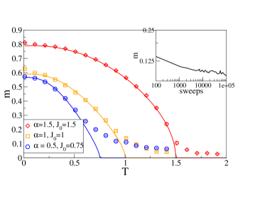
Figure 1: The magnetization $m$ as a function of the temperature $T$ for several values of $\alpha$ and $J_{0}$. Simulation results (markers) are compared with results from the theory (solid lines) for $J_{1}=1$, $\gamma=0$. At low temperatures theory and simulations are in good agreement. Because of the increase in the equilibration time around the critical temperature the results from simulation overestimate the magnetization. The inset confirms this: it shows the value of the magnetization as a function of the number of Monte Carlo sweeps for $\alpha=0.5,J_{0}=0.75$ and $T=1$.

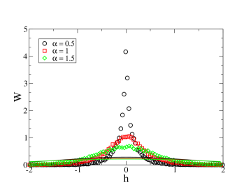
Figure 2: The distribution of effective fields with $J_{0}=\gamma=0$, $J_{1}=1$, $T=0.4$ and several values of $\alpha$. The markers give the distributions according to equation (21) while the solid lines are obtained through the theory of [15]. All the moments of the distributions are finite. Therefore we have leptokurtic distributions which are neither Gaussian nor Lévy distributions.

4 Cavity method

We derive the self-consistent eqs. (21) for $W(h)$ through the cavity method. In contrast with [15] we only apply the CLT to the field coming from the weak bonds, i.e. bonds smaller than the cutoff $T\epsilon$. The bonds larger than $T\epsilon$ form a backbone graph of strong bonds which is treated as a FiC system. For $\epsilon\rightarrow\infty$ we find back the results of [15]. For $\epsilon\rightarrow 0$ we expect to find the RS behavior of the spin glass.

The marginal $P_{i}(\sigma_{i})\equiv\sum_{\left\{\sigma_{j}\right\}_{j=1..N}\setminus\sigma_{i}}P\left(\left\{\sigma_{j}\right\}_{j=1..N}\right)$ of the Gibbs distribution $P\left(\left\{\sigma_{j}\right\}_{j=1..N}\right)\sim\exp\left[-\beta H\left(\left\{\sigma_{j}\right\}_{j=1..N}\right)\right]$ can be written as

$$P_{i}(\sigma_{i}) \sim\sum_{\left\{\sigma_{j}\right\}_{j=1..N}\setminus\sigma_{i}}P^{(i)}\left(\left\{\sigma_{j}\right\}_{j=1..N}\setminus\sigma_{i}\right)\exp\left(\sum_{k}J_{ki}\sigma_{j}\sigma_{i}\right),$$ (24)

with $P^{(i)}\left(\left\{\sigma_{j}\right\}_{j=1..N}\setminus\sigma_{i}\right)$ the Gibbs distribution on the cavity graph $G^{(i)}$. The cavity graph is the subgraph of the original graph $G$ where one removed the $i$-th spin and all of its interactions with the other spins. We assume that the probability distribution on the cavity graph factorizes [3]:

$$P^{(i)}\left(\left\{\sigma_{j}\right\}_{j=1..N}\setminus\sigma_{i}\right)=\prod_{j(\neq i)}P^{(i)}_{j}(\sigma_{j}).$$ (25)

This factorization is valid when there is one pure phase in the system. The set $\overline{\omega}^{(i)}$ of all weak bonds and the set $\omega^{(i)}$ of all strong bonds are defined through:

$$\overline{\omega}^{(i)}\equiv\left\{j\in\mathbb{N}\cap[1,N]|J_{ij}<T\epsilon\right\},$$ (26)

$$\omega^{(i)}\equiv(\mathbb{N}\cap[1,N])\setminus\overline{\omega}^{(i)}.$$ (27)

The cavity fields $h^{(i)}_{j}$ and $g^{(i)}_{j}$ are defined through:

$$h^{(i)}_{j}\equiv\sum_{\sigma}\frac{\sigma}{2}\log\left(P^{(i)}_{j}(\sigma)\right) \rm{if} j\in\omega^{(i)},$$ (28)

$$g^{(i)}_{j}\equiv\sum_{\sigma}\frac{\sigma}{2}\log\left(P^{(i)}_{j}(\sigma)\right) \rm{if} j\in\overline{\omega}^{(i)}.$$ (29)

The marginal $P^{(j)}_{i}$ of the $i$-th spin on the cavity graph $G^{(j)}$ is equal to:

$$P^{(j)}_{i}(\sigma_{i})\sim\prod_{k\in\overline{\omega}^{(i)}\setminus j}\sum_{\tau}\exp\left(\beta J_{ki}\sigma_{i}\tau+\beta g^{(i)}_{k}\tau\right)\prod_{k\in\omega^{(i)}\setminus j}\sum_{\tau}\exp\left(\beta J_{ki}\sigma_{i}\tau+\beta h^{(i)}_{k}\tau\right).$$ (30)

We used the notation $h^{(j)}_{i}$ for cavity fields where one removed a site $j$ connected with $i$ through a strong bond and the notation $g^{(j)}_{i}$ for fields where the site $j$ was connected with $i$ through a weak bond . We thus find the following set of closed equations in the cavity fields $h^{(j)}_{i}$ and $g^{(j)}_{i}$:

$$g^{(j)}_{i}=z^{(j)}_{i}+\beta^{-1}\sum_{k\in\omega_{i}}{\rm{atanh}}\left(\tanh\left(\beta h^{(i)}_{k}\right)\tanh\left(\beta J_{ki}\right)\right),$$ (31)

$$h^{(j)}_{i}=z_{i}+\beta^{-1}\sum_{k\in\omega_{i}\setminus j}{\rm{atanh}}\left(\tanh\left(\beta h^{(i)}_{k}\right)\tanh\left(\beta J_{ki}\right)\right),$$ (32)

where we defined a third field containing the contributions from the weak bonds

$$z^{(j)}_{i}=\beta^{-1}\sum_{k\in\overline{\omega}_{i}\setminus j}{\rm{atanh}}\left(\tanh\left(\beta g^{(i)}_{k}\right)\tanh\left(\beta J_{ki}\right)\right).$$ (33)

In the limit $N\rightarrow\infty$ we can remove the $j$ dependency in the fields $z^{(j)}_{i}$ and $g^{(j)}_{i}$ because the sum over the weak bonds ($k\in\overline{\omega_{i}}$) contains an infinite number of terms.

To take the disorder average over the couplings we define the following distributions:

$$W_{\rm{w}}(g)\equiv\overline{\frac{\sum^{N}_{i=1}\delta\left(g-g_{i}\right)}{N}},$$ (34)

$$W_{\rm{s}}(h)\equiv\overline{\frac{\sum^{N}_{i=1}\sum_{j\in\omega_{i}}\delta\left(h-h^{(j)}_{i}\right)}{\sum^{N}_{i=1}\sum_{j\in\omega_{i}}}},$$ (35)

$$W_{\rm g}(z)\equiv\overline{\frac{\sum^{N}_{i=1}\delta(z-z_{i})}{N}}.$$ (36)

We treat the $z$-fields as a sum of infinitely many random variables on which we can apply the CLT:

$$W_{\rm g}(z)=\frac{1}{\sqrt{4\pi\Delta q}}\exp\left(-\frac{(z-\tilde{J_{0}}m)^{2}}{4\Delta q}\right),$$ (37)

with $\Delta$ and $\tilde{J}_{0}$ as defined in eqs. (22) and (23). The parameters $m$ and $q$ determine, respectively, the mean and the variance of the Gaussian distribution $W_{\rm g}(z)$. Here is the important difference with [15] where the CLT is applied on all bonds, also on the strong ones.

From eq. (33) one finds, for $N\rightarrow\infty$ and $\epsilon\ll 1$ the following expressions for the mean $m$ and the variance $q$

$$m=\left(\tilde{J}_{0}\right)^{-1}\left(N\int^{T\epsilon}_{-T\epsilon}dJP^{J_{1},\gamma,J_{0}}_{\alpha}(J)J\right)\int dg\tanh(\beta g)W_{\rm w}(g),$$ (38)

$$q=\left(2\Delta\right)^{-1}\left(N\int^{T\epsilon}_{-T\epsilon}dJP^{J_{1},\gamma,J_{0}}_{\alpha}(J)J^{2}\right)\int dg\tanh^{2}(\beta g)W_{\rm w}(g).$$ (39)

The integrals over the couplings in eqs. (38) and (39) can be calculated using analogous methods as used to derive the integrals in appendix B:

$$N\int^{T\epsilon}_{-T\epsilon}dJP^{J_{1},\gamma,J_{0}}_{\alpha}(J)J=\tilde{J}_{0},$$ (40)

$$N\int^{T\epsilon}_{-T\epsilon}dJP^{J_{1},\gamma,J_{0}}_{\alpha}(J)J^{2}=2\Delta.$$ (41)

Using the definitions of the distributions $W_{\rm{w}}(g)$ and $W_{\rm{s}}(h)$ in eqs. (34) and (35) we get

$$W_{\rm s}(h) =\sum^{\infty}_{k=0}\frac{p_{\rm poiss}(k;c)k}{c}\prod^{k-1}_{r=1}\int dh_{r}W_{\rm s}(h_{r})\int\prod^{k-1}_{r=1}dJ_{r}P_{\epsilon}(J_{r})\int dzW_{\rm g}(z)$$ (42)

$$\delta\left(h-z-\beta^{-1}\sum^{k-1}_{r=1}{\rm{atanh}}\left(\tanh(\beta h_{r})\tanh(\beta J_{r})\right)\right),$$

$$W_{\rm w}(g) =\sum^{\infty}_{k=0}p_{\rm poiss}(k;c)\int\prod^{k}_{r=1}dh_{r}W_{\rm s}(h_{r})\int\prod^{k}_{r=1}dJ_{r}P_{\epsilon}(J_{r})\int dzW_{\rm g}(z)$$ (43)

$$\delta\left(g-z-\beta^{-1}\sum^{k}_{r=1}{\rm{atanh}}\left(\tanh(\beta h_{r})\tanh(\beta J_{r})\right)\right).$$

The mean connectivity $c$ is given by

$$c=\lim_{N\rightarrow\infty}\frac{\sum^{N}_{i=1}|\omega^{(i)}(\epsilon)|}{N}=\int^{\infty}_{T\epsilon}dJ\rho(J)+\int^{-T\epsilon}_{-\infty}dJ\rho(J)=\frac{2C_{\alpha}}{\alpha(T\epsilon)^{\alpha}},$$ (44)

with $\rho(J)$ the large tail behavior as defined in (4). We use the following property of Poissonian distributions: $\frac{1}{c}p_{\rm poiss}(k;c)k=p_{\rm poiss}(k-1;c)$ to find $W_{\rm w}(g)=W_{\rm s}(g)=W_{\epsilon}(g)$, i.e. the solutions to (42) and (43) are the same as the solution $W_{\epsilon}$ of (21). Indeed, eqs. (43) combined with (38) and (39) are identical to eqs. (17) and (21) derived with the replica method. From the cavity approach the importance of the CLT in Lévy spin glasses becomes clear: the couplings have a divergent variance, therefore one can not apply the CLT as done in [15]. We remark that the effective coupling $\tilde{J}_{0}$ and the parameter $2\Delta$ appearing in the replica method are the mean and the variance of the weak couplings. The distribution $W_{\epsilon}(h)$ in equations (21) is the distribution of the cavity fields propagating along the backbone graph of strong bonds.

5 Stability of the replica symmetric ansatz

As is known [24], the RS ansatz introduced in (12) is unstable at low temperatures. It is possible to calculate the regions of stability by using the two replica method, first introduced for FiC models in [25]. This method allows us to study local and non-local replica symmetry breaking (RSB) effects. For models on graphs a relevant instability condition is proved rigorously in [26]. It determines the region where the message passing algorithms stop to converge, see for example the discussion in [27].

We start by considering two uncoupled replicas. Both replicas fulfill the equations (30)-(33). The replicas only get coupled when we take the average over the graph instance. Indeed, the effective field distribution of two sets of uncoupled spins on the same graph with the same couplings is given by:

$$W_{\epsilon}(h^{1},h^{2}) =\sum^{\infty}_{k=0}\frac{p_{\rm poiss}(k;c)k}{c}\prod^{k-1}_{r=1}\int dh^{1}_{r}dh^{2}_{r}W_{\epsilon}(h^{1}_{r},h^{2}_{r})\int\prod^{k-1}_{r=1}dJ_{r}P_{\epsilon}(J_{r})\int dz^{1}dz^{2}W_{\rm g}(z^{1},z^{2})$$ (45)

$$\times\delta\left(h^{1}-z^{1}-\beta^{-1}\sum^{k-1}_{r=1}{\rm{atanh}}\left(\tanh(\beta h^{1}_{r})\tanh(\beta J_{r})\right)\right)$$

$$\times\delta\left(h^{2}-z^{2}-\beta^{-1}\sum^{k-1}_{r=1}{\rm{atanh}}\left(\tanh(\beta h^{2}_{r})\tanh(\beta J_{r})\right)\right).$$

We assume again that we can apply the CLT on the $z$-fields:

$$W_{\rm g}(z^{1},z^{2})$$

$$=\frac{1}{4\Delta\pi\sqrt{q^{1}q^{2}(1-\rho^{2})}}\exp\left(-\frac{1}{2(1-\rho^{2})}\left(\frac{(z^{1}-\tilde{J}_{0}m^{1})^{2}}{2\Delta q^{1}}+\frac{(z^{2}-\tilde{J}_{0}m^{2})^{2}}{2\Delta q^{2}}\right)\right)$$

$$\times\exp\left(\frac{\rho(z^{1}-\tilde{J}_{0}m^{1})(z^{2}-\tilde{J}_{0}m^{2})}{2(1-\rho^{2})\Delta\sqrt{q^{1}q^{2}}}\right).$$ (46)

The order parameters become

$$m^{1}=\int dg^{1}dg^{2}\tanh(\beta g^{1})W_{\epsilon}(g^{1},g^{2}),$$ (47)

$$q^{1}=\int dg^{1}dg^{2}\tanh^{2}(\beta g^{1})W_{\epsilon}(g^{1},g^{2}),$$ (48)

$$m^{2}=\int dg^{1}dg^{2}\tanh(\beta g^{2})W_{\epsilon}(g^{1},g^{2}),$$ (49)

$$q^{2}=\int dg^{1}dg^{2}\tanh^{2}(\beta g^{2})W_{\epsilon}(g^{1},g^{2}),$$ (50)

$$\rho\sqrt{q^{1}q^{2}}=\int dg^{1}dg^{2}\tanh(\beta g^{2})\tanh(\beta g^{1})W_{\epsilon}(g^{1},g^{2}).$$ (51)

In the limit $\alpha\rightarrow 2$ we find $W_{\epsilon}(h^{1},h^{2})=W_{\rm g}(h^{1},h^{2})$. An expansion around the RS solution $m^{1}=m^{2}=m$, $q^{1}=q^{2}=q$ and $1-|\rho|\sim\mathcal{O}(\delta)$, with $\delta\ll 1$, leads to the following stability condition:

$$\beta^{-2}=\int^{+\infty}_{-\infty}\frac{du}{\sqrt{2\pi}}\exp\left(-\frac{u^{2}}{2}\right)\mathrm{sech}^{4}\left(\beta\sqrt{q}u+\beta J_{0}m\right).$$ (52)

The parameters $(q,m)$ in (52) are, respectively, the overlap parameter and the magnetization of the SK model. Equation (52) is precisely the AT line of the SK model, see [24].

6 Phase Diagram

The system shows three phases which depend on the values of the order parameters $m$ and $q$ defined in (17): a paramagnetic phase (P) with $m=q=0$, a ferromagnetic phase (F) with $m>0,q>0$ and a spin-glass phase (SG) with $m=0,q>0$.

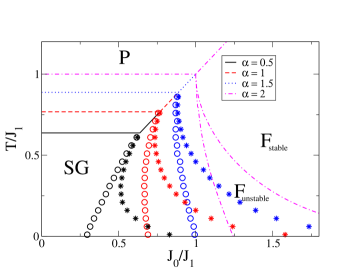
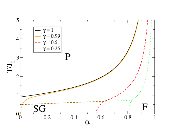
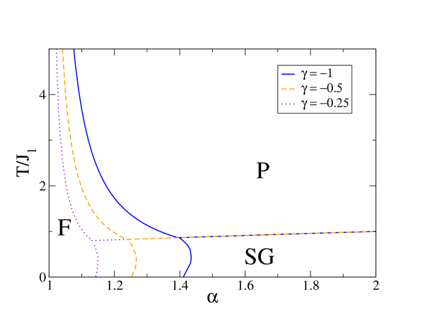
Figure 3: The $(T/J_{1},J_{0}/J_{1})$ phase diagram for several values of $\alpha$ and with a skewness $\gamma=0$. Three phases appear: P (paramagnetic), F (ferromagnetic) and SG (spin glass). The circles present the SG-F transitions and the stars indicate where the F phase becomes stable against replica symmetry breaking. For $\alpha=2$ the phase diagram coincides with that of the SK model.

Figure 4: The $(T/J_{1},\alpha)$ phase diagrams for different values of the skewness $\gamma$ and a shift $J_{0}=0$. The figure on the left gives the phase diagram for $\gamma>0$ while the figure on the right gives the phase diagram for $\gamma<0$. For $\gamma=1$ and $\alpha<1$ there is no SG phase. The $P-SG$ transition is independent of $\gamma$. For $\gamma=0.99$ the dashed part of the transition line does not present the SG-F transition but the instability line of the P phase with respect to the F phase.

The ferromagnetic phase contains a region stable to RSB effects ($F_{\rm stable}$) and a region unstable to RSB effects $(F_{\rm unstable})$.

The P-F and P-SG transitions are determined using an expansion of the self-consistent eq. (21) around the paramagnetic solution $W_{\epsilon}(h)=\delta(h)$. For $\gamma=0$ we find the same bifurcation lines as derived in [17]. To determine the SG-F transition and the $F_{\rm unstable}$ to $F_{\rm stable}$ transition one has to solve numerically, respectively, eqs. (21) and (45) with for instance a population dynamics algorithm.

In figure 4 the different phases in the $(J_{0}/J_{1},T/J_{1})$ phase diagram are presented for a skewness $\gamma=0$ and several values of $\alpha$. The open circles present the SG-F transitions and the stars mark the points where the F phase becomes stable with respect to RSB. These results generalize the phase diagram obtained in the seminal paper of Sherrington and Kirkpatrick [1] to coupling distributions with a large tail. For $\gamma=0$ the P-F transition is independent of $\alpha$. When $\alpha$ increases the SG phase increases in favor of a smaller F phase. The RSB effects decrease when $\alpha$ decreases: indeed the $F_{\rm unstable}$ becomes smaller and the reentrance effect in the SG-F phase transition line diminishes and finally disappears. This is related to the decrease of frustration due to the presence of stronger bonds that dominate the systems behavior. We did not find a replica symmetric SG phase (i.e., a SG phase stable with respect to RSB), contrary to the conjecture made in [15]. Replica symmetry breaks continuously at the SG transition similar to the behavior of the SK model. We did not find any further evidence for the conjecture in [15] that replica symmetry restores at $T=0$.

In figure 4 we present the $(T/J_{1},\alpha)$-phase diagram for different values of $\gamma$ and $J_{0}=0$. We consider the following regions:

• $\gamma>0$ and $\alpha<1$ (left figure): the F phase increases and the SG phase decreases as a function of increasing $\gamma$. The SG phase disappears at $\gamma=1$. For values of $\gamma$ very close to one the SG phase is only present for very small values of $\alpha$. The transition temperature between the P and F phase becomes infinite for $\alpha\rightarrow 1^{-}$.

• $\gamma<0$ and $\alpha>1$ (right figure): the F phase decreases and the SG phase increases as a function of increasing $\gamma$. The transition temperature between the P and F phase becomes infinite for $\alpha\rightarrow 1^{+}$.

• $\gamma>0$ and $\alpha>1$ (not shown): there is no F phase but a P and SG phase.

• $\gamma<0$ and $\alpha<1$ (not shown): there is no F phase but a P and SG phase.

We have some additional remarks: The transition temperature becomes very large for $\alpha\rightarrow 1^{\pm}$ (for, respectively, $\gamma<0$ and $\gamma>0$) because the effective coupling $\tilde{J}_{0}\rightarrow\infty$. There is no SG phase for $\gamma=1$ and $\alpha<1$ because there are no negative couplings, only the P-F transition occurs. The P-SG transitions coincide for different values of $\gamma$. For low values of $\alpha$ the results of population dynamics become inaccurate because of numerical imprecisions when dealing with a broad range of coupling values. In this case we used the instability line of the P phase with respect to the F phase as of the location of the SG-F transition.

7 Entropy

It is possible to calculate the free energy from the saddle point equations. We use the RS ansatz and we introduce again a cutoff $\epsilon$. The entropy is given by $s=\beta^{2}\frac{\partial f}{\partial\beta}=\lim_{\epsilon\rightarrow 0}s(\epsilon)$ with $s(\epsilon)$:

$$s(\epsilon)=\beta^{2}\frac{\Delta}{2}\left(1-q^{2}\right)-\beta^{2}\Delta\left(1-q\right)+s_{\rm site}(\epsilon)-\frac{c}{2}s_{\rm link}(\epsilon).$$ (53)

The quantity $s_{\rm link}$ is equal to

$$s_{\rm link}(\epsilon) =-\int dhdh^{\prime}W_{\epsilon}(h)W_{\epsilon}(h^{\prime})\int dJP_{\epsilon}(J)$$ (54)

$$\sum_{\sigma,\tau}\frac{\exp\left(\beta J\sigma\tau+\beta h\sigma+\beta h^{\prime}\tau\right)}{\sum_{\sigma,\tau}\exp\left(\beta J\sigma\tau+\beta h\sigma+\beta h^{\prime}\tau\right)}\log\left(\frac{\exp\left(\beta J\sigma\tau+\beta h\sigma+\beta h^{\prime}\tau\right)}{\sum_{\sigma,\tau}\exp\left(\beta J\sigma\tau+\beta h\sigma+\beta h^{\prime}\tau\right)}\right),$$

and $s_{\rm site}$ reads

$$s_{\rm site}(\epsilon) =-\sum_{k=0}^{\infty}\frac{c^{k}e^{-c}}{k!}\prod_{l=1}^{k}\biggl{[}\int dh_{l}W_{\epsilon}(h_{l})\int dJ_{l}P_{\epsilon}(J_{l})\biggr{]}\int\mathcal{D}z$$ (55)

$$\sum_{\sigma;(\tau_{1},\tau_{2},\cdots,\tau_{k})}\frac{\exp\left((\beta J_{0}m+\sqrt{2q\Delta}z)\sigma\right)\prod^{k}_{\ell=1}\left(\exp\left(\beta J_{\ell}\tau_{\ell}\sigma\right)\exp\left(\beta h_{\ell}\tau_{\ell}\right)\right)}{\sum_{\sigma;(\tau_{1},\tau_{2},\cdots,\tau_{k})}\exp\left((\beta J_{0}m+\sqrt{2q\Delta}z)\sigma\right)\prod^{k}_{\ell=1}\left(\exp\left(\beta J_{\ell}\tau_{\ell}\sigma\right)\exp\left(\beta h_{\ell}\tau_{\ell}\right)\right)}$$

$$\log\left[\frac{\exp\left((\beta J_{0}m+\sqrt{2q\Delta}z)\sigma\right)\prod^{k}_{\ell=1}\left(\exp\left(\beta J_{\ell}\tau_{\ell}\sigma\right)\exp\left(\beta h_{\ell}\tau_{\ell}\right)\right)}{\sum_{\sigma;(\tau_{1},\tau_{2},\cdots,\tau_{k})}\exp\left((\beta J_{0}m+\sqrt{2q\Delta}z)\sigma\right)\prod^{k}_{\ell=1}\left(\exp\left(\beta J_{\ell}\tau_{\ell}\sigma\right)\exp\left(\beta h_{\ell}\tau_{\ell}\right)\right)}\right].$$

For $\alpha\rightarrow 2$ one gets precisely the entropy of the SK model [2]. The entropies $s_{\rm site}$ and $s_{\rm link}$ correspond with the entropy differences when performing, respectively, a site addition and a link addition on the backbone graph of strong bonds, see [19, 23]. Similar to the form of the self-consistent equation (21) for $W_{\epsilon}(h)$ we find that the entropy as given by equation (53) corresponds to the entropy of an Ising model on a Poissonian graph with mean connectivity $c$, a distribution of the bonds $P_{\epsilon}$ and an extra Gaussian noise $z$.

We plotted the entropy $s$ as a function of $\alpha$ in figure 5. From this figure we see that the entropy gets less negative, for $T\rightarrow 0$. We find that for smaller values of $\alpha\lesssim 1$ the entropy becomes eventually zero for $T\rightarrow 0$. This is consistent with a decrease of RSB effects when $\alpha$ decreases.

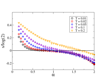
Figure 5: The entropy $s$ as a function of the exponent $\alpha$ for different values of the temperature $T$, $J_{0}=0$, $\gamma=0$ and $J_{1}=1$. The filled markers at $\alpha=2$ show the SK values. The entropy converges to the SK value for $\alpha\rightarrow 2$.

8 Conclusion

In this paper we have shown how to derive the phase diagrams of Lévy spin glasses where the couplings between the spins are drawn from a distribution with power law tails characterized by an exponent $\alpha$. These models are known to have a finite number of strong bonds of order $\mathcal{O}(1)$ and an infinite amount of weak bonds of order $\mathcal{O}(N^{-1/\alpha})$. The crucial difference with previous works [15] and [17] is that we derive the phase diagrams, the entropy and the stability against replica symmetry of Lévy spin glasses without using the Gaussian assumption for the distribution of fields. We have neither found evidence for a replica symmetric spin-glass phase, nor for a restoration of the replica symmetry at zero temperature, contrary to the conjecture in [15]. We have solved the problem using the replica and the cavity method within, respectively, the replica symmetric assumption and the assumption of one pure phase. The resultant effective equations for the distribution of cavity fields show clearly the hybrid character of the model being a mixture between a finite connectivity model and a fully connected model.

The phase transitions are qualitatively similar to the ones found in the SK model. Large tails do influence quantitatively the phase diagram: the Lévy spin-glass model becomes more stable with respect to replica symmetry breaking and the SG phase decreases when the tails get larger. Moreover, the reentrance effects in the replica symmetric phase diagram disappear for $\alpha\lesssim 1$. The replica symmetry breaking transitions are all continuous. The skewness $\gamma$ in the Lévy distribution can have a big influence on the size of the F phase. For $\alpha\rightarrow 2$ the effective distribution of fields becomes Gaussian and we have found back the results of the SK model. For $\alpha<2$ this distribution is neither Lévy nor Gaussian, but a distribution with finite moments and a kurtosis smaller than a Gaussian with the same variance.

Appendix A Stable distributions

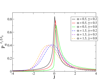
Figure 6: The Lévy distributions $P^{J_{1},\gamma,J_{0}}_{\alpha}(J)$ for $J_{1}=1$, $J_{0}=0$ and different values of $\alpha$ and $\gamma$. The distributions with $\alpha=1.5$ approach a Gaussian while the ones for $\alpha=0.5$ have larger tails. For $\gamma>0$, the center of the distribution goes to $+\infty$ or $-\infty$ for $\alpha\uparrow 1$ or $\alpha\downarrow 1$, respectively. The coupling distribution fulfills $P^{J_{1},\gamma,J_{0}}_{\alpha}(J)=P^{J_{1},-\gamma,J_{0}}_{\alpha}(-J)$.

The purpose of this appendix is to give some intuition on the role of the parameters $\alpha$ and $\gamma$ present in stable distributions, defined through eqs. (2) and (3). Both $\alpha$ and $\gamma$ are responsible for the shape of the distribution. The main role of the exponent $\alpha$ is to control the decay of the tails. Figure 6 shows that, for a fixed $\gamma$, a decrease in $\alpha$ gives rise to a distribution $P^{J_{1},\gamma,J_{0}}_{\alpha}(J)$ with larger tails and more sharply peaked around its most probable value $J$. The center of $P^{J_{1},\gamma,J_{0}}_{\alpha}(J)$ is also shifted from the negative to the positive J-axis as $\alpha$ decreases from $\alpha>1$ to $\alpha<1$. A change of $\alpha$ has no effect on the position of the center when $\gamma=0$.

The skewness parameter $\gamma$ controls the relative weight between the positive and negative tails. For $\gamma>0$, the positive tail of $P^{J_{1},\gamma,J_{0}}_{\alpha}(J)$ is larger than the negative one; for $\gamma<0$ vica versa. The distribution is symmetric around $J_{0}$ when $\gamma=0$. For increasing positive values of $\gamma$, see figure 6, the center of $P^{J_{1},\gamma,J_{0}}_{\alpha}(J)$ shifts to the right or left provided $\alpha<1$ or $\alpha>1$, respectively.

Appendix B Solution of integrals

In this appendix we show how to integrate over $\hat{J}$ in the following equations:

$$I_{1} = \int_{-\infty}^{\infty}\frac{dJd\hat{J}}{2\pi}|\hat{J}|^{\alpha}e^{i\hat{J}J}f(J),$$ (56)

$$I_{2} = \int_{-\infty}^{\infty}\frac{dJd\hat{J}}{2\pi}|\hat{J}|^{\alpha}{\rm sign}(\hat{J})e^{i\hat{J}J}f(J),$$ (57)

where $f(J)$ is given by eq. (14) and $\alpha\in(0,1)\cup(1,2]$. We obtained the following results for $I_{1}$ and $I_{2}$ after integration over $\hat{J}$

$$I_{1}=-\left(\frac{\sqrt{2}}{J_{1}}\right)^{\alpha}C_{\alpha}\int_{-\infty}^{\infty}\frac{dJ}{|J|^{\alpha+1}}\Big{[}f(J)-f(0)\Big{]},{\rm if}\quad 0<\alpha<2,$$ (58)

$$I_{2} =i\left(\frac{\sqrt{2}}{J_{1}}\right)^{\alpha}\frac{C_{\alpha}}{\Phi}\int_{-\infty}^{\infty}\frac{dJ}{|J|^{\alpha+1}}{\rm sign}(J)f(J),{\rm if}\quad 0<\alpha<1,$$ (59)

$$=i\left(\frac{\sqrt{2}}{J_{1}}\right)^{\alpha}\frac{C_{\alpha}}{\Phi}\int_{-\infty}^{\infty}\frac{dJ}{|J|^{\alpha+1}}{\rm sign}(J)\Big{[}f(J)-f^{\prime}(0)J\Big{]},{\rm if}\quad 1<\alpha\leq 2,$$ (60)

where the parameters $C_{\alpha}$ and $\Phi$ are defined in section 2. We have left out the dependence of $f(J)$ with respect to $h$ and $s$ since it is not important here. The aim of this appendix is to show how one can derive eqs. (58), (59) and (60) from eqs. (56) and (57).

By introducing an exponential convergence factor in eqs. (56) and (57), we can rewrite them as follows

$$I_{1} = \lim_{a\rightarrow 0^{+}}\int_{0}^{\infty}dJ\Big{[}f(J)+f(-J)\Big{]}\int_{0}^{\infty}\frac{d\hat{J}}{\pi}\hat{J}^{\alpha}\cos{(\hat{J}J)}e^{-a\hat{J}},$$ (61)

$$I_{2} = i\lim_{a\rightarrow 0^{+}}\int_{0}^{\infty}dJ\Big{[}f(J)-f(-J)\Big{]}\int_{0}^{\infty}\frac{d\hat{J}}{\pi}\hat{J}^{\alpha}\sin{(\hat{J}J)}e^{-a\hat{J}}.$$ (62)

The integrals over $\hat{J}$ are calculated for $a>0$ and, afterwards, the limit $a\rightarrow 0$ is performed. Reference [28] can be used in order to integrate over $\hat{J}$ in eqs. (61) and (62), giving rise to

$$I_{1} = \frac{\Gamma(\alpha+1)}{\pi}\lim_{a\rightarrow 0^{+}}\int_{0}^{\infty}dJ\Big{[}f(J)+f(-J)\Big{]}\frac{\cos{\Big{[}(\alpha+1){\rm arctan}(\frac{J}{a})\Big{]}}}{(J^{2}+a^{2})^{\frac{\alpha+1}{2}}},$$ (63)

$$I_{2} = i\frac{\Gamma(\alpha+1)}{\pi}\lim_{a\rightarrow 0^{+}}\int_{0}^{\infty}dJ\Big{[}f(J)-f(-J)\Big{]}\frac{\sin{\Big{[}(\alpha+1){\rm arctan}(\frac{J}{a})\Big{]}}}{(J^{2}+a^{2})^{\frac{\alpha+1}{2}}}.$$ (64)

In order to analyze the behavior of integrals (63) and (64) around $J=0$ when $a\rightarrow 0^{+}$, we insert a cutoff $\lambda>0$ and split them as follows

$$I_{1} =\frac{\Gamma(\alpha+1)}{\pi}U_{1}(\lambda)+\frac{\Gamma(\alpha+1)}{\pi}\cos{\Big{[}(\alpha+1)\frac{\pi}{2}\Big{]}}\int_{\lambda}^{\infty}\frac{dJ}{J^{\alpha+1}}\Big{[}f(J)+f(-J)\Big{]},$$ (65)

$$I_{2} =i\frac{\Gamma(\alpha+1)}{\pi}U_{2}(\lambda)+i\frac{\Gamma(\alpha+1)}{\pi}\sin{\Big{[}(\alpha+1)\frac{\pi}{2}\Big{]}}\int_{\lambda}^{\infty}\frac{dJ}{J^{\alpha+1}}\Big{[}f(J)-f(-J)\Big{]},$$ (66)

where

$$U_{1}(\lambda)=\lim_{a\rightarrow 0^{+}}\int_{0}^{\lambda}\frac{dJ}{a^{\alpha+1}}\Big{[}f(J)+f(-J)\Big{]}\frac{\cos{\Big{[}(\alpha+1){\rm arctan}(\frac{J}{a})\Big{]}}}{\Big{[}\Big{(}\frac{J}{a}\Big{)}^{2}+1\Big{]}^{\frac{\alpha+1}{2}}},$$ (67)

$$U_{2}(\lambda)=\lim_{a\rightarrow 0^{+}}\int_{0}^{\lambda}\frac{dJ}{a^{\alpha+1}}\Big{[}f(J)-f(-J)\Big{]}\frac{\sin{\Big{[}(\alpha+1){\rm arctan}(\frac{J}{a})\Big{]}}}{\Big{[}\Big{(}\frac{J}{a}\Big{)}^{2}+1\Big{]}^{\frac{\alpha+1}{2}}}.$$ (68)

The limit $a\rightarrow 0^{+}$ has been performed on the right hand side of eqs. (65) and (66). The integrals present in the definition of $U_{1}(\lambda)$ and $U_{2}(\lambda)$ are computed through a power-series representation of their integrands, yielding the results

$$U_{1}(\lambda) = \lim_{a\rightarrow 0^{+}}\sum_{n,l=0}^{\infty}u_{nl}\,\Big{(}\frac{\lambda}{a}\Big{)}^{2l+\alpha+1}\lambda^{2n-\alpha},$$ (69)

$$U_{2}(\lambda) = \lim_{a\rightarrow 0^{+}}\sum_{n,l=0}^{\infty}v_{nl}\,\Big{(}\frac{\lambda}{a}\Big{)}^{2l+\alpha+2}\lambda^{2n+1-\alpha}.$$ (70)

The explicit forms of the coefficients $\{u_{nl}\}$ and $\{v_{nl}\}$ are irrelevant. The analysis of eqs. (65) and (66) as $\lambda$ tends to zero, constrained to the limit $a\rightarrow 0^{+}$ in the functions $U_{1}(\lambda)$ and $U_{2}(\lambda)$, constitutes the final step of the calculation.

One can notice from eq. (69) that $U_{1}(\lambda)$ diverges for $\lambda\rightarrow 0^{+}$. However, the transformation of $f(J)$ according to $f(J)\rightarrow f(J)-f(0)$ removes this divergence and makes $U_{1}(\lambda)$ go to zero for $\lambda\rightarrow 0^{+}$, provided that $\alpha<2$. This allows us to perform the limit $\lambda\rightarrow 0^{+}$ in eq. (65) which leads, after comparison with eq. (56), to the following result

$$\int_{-\infty}^{\infty}\frac{dJd\hat{J}}{2\pi}|\hat{J}|^{\alpha}e^{i\hat{J}J}\Big{[}f(J)-f(0)\Big{]}=-\frac{\Gamma(\alpha+1)}{\pi}\sin{\Big{(}\frac{\alpha\pi}{2}\Big{)}}$$

$$\times\int_{0}^{\infty}\frac{dJ}{J^{\alpha+1}}\Big{[}f(J)+f(-J)-2f(0)\Big{]},\,0<\alpha<2.$$ (71)

By integrating the term with $f(0)$ on the left hand side of the above equation we get eq. (58).

The calculation of eqs. (59) and (60) proceeds in an analogous way. Depending on the value of $\alpha$, there are two different situations concerning the behavior of eq. (70) for $\lambda\rightarrow 0^{+}$. For $\alpha<1$, we obtain $\lim_{\lambda\rightarrow 0^{+}}U_{2}(\lambda)=0$, which allows to perform the limit $\lambda\rightarrow 0^{+}$ in eq. (66). For $\alpha>1$, it is necessary to transform $f(J)$ according to $f(J)\rightarrow f(J)-f^{\prime}(0)J$ in order to obtain $\lim_{\lambda\rightarrow 0^{+}}U_{2}(\lambda)=0$ and to perform the limit $\lambda\rightarrow 0^{+}$ in eq. (66).

References

References

- [1] D. Sherrington and S. Kirkpatrick, “Solvable model of a spin-glass,” Phys. Rev. Lett., vol. 35, p. 1792, 1975.
- [2] S. Kirkpatrick and D. Sherrington, “Infinite-ranged models of spin-glasses,” Phys. Rev. B, vol. 17, p. 4384, 1978.
- [3] M. Mézard, G. Parisi, and M. A. Virasoro, Spin Glass Theory and Beyond, vol. 9 of World Scientific Lecture Notes in Physics. World Scientific Pub Co Inc., 1987.
- [4] M. W. Klein, “Temperature-dependent internal field distribution and magnetic susceptibility of a dilute ising spin system,” Phys. Rev., vol. 173, p. 552, 1968.
- [5] M. W. Klein, C. Held, and E. Zuroff, “Dipole interactions among polar defects: A self-consistent theory with application to impurities in kcl,” Phys. Rev. B, vol. 13, p. 3576, 1976.
- [6] D. V. Berkov, “Local-field distribution in systems with dipolar interparticle interaction,” Phys. Rev. B, vol. 53, p. 731, 1996.
- [7] P. Lévy, Theory de l’addition de Variables Aléatoires. Paris: Gauthier-Villars, 1937.
- [8] B. V. Gnedenko and A. N. Kolmogorov, Limit Distributions for Sums of Independent Random Variables. Cambridge: Addison-Wesley, 1954.
- [9] G. Biroli, J. P. Bouchaud, and M. Potters, “Extreme value problems in random matrix theory and other disordered systems,” J. Stat. Mech., p. 07019, 2007.
- [10] P. Cizeau and J. P. Bouchaud, “Theory of lévy matrices,” Phys. Rev. E, vol. 50, p. 1810, 1994.
- [11] Z. Burda, J. Jurkiewicz, M. A. Nowak, G. Papp, and I. Zahed, “Free random lévy and wigner-lévy matrices,” Phys. Rev. E, vol. 75, p. 051126, 2007.
- [12] G. Biroli, J. P. Bouchaud, and M. Potters, “On the top eigenvalue of heavy-tailed random matrices,” Eur. Phys. Lett., vol. 78, p. 10001, 2007.
- [13] J. P. Bouchaud and A. Georges, “Anomalous diffusion in random media: statistical mechanisms, models and physical applications,” Phys. Rep., vol. 195, p. 127, 1990.
- [14] S. Galluccio, J. P. Bouchaud, and M. Potters, “Rational decisions, random matrices and spin glasses,” Physica A, vol. 259, p. 449, 1998.
- [15] P. Cizeau and J.-P. Bouchaud, “Mean field theory of dilute spin-glasses with power-law interactions,” J. Phys. A: Math. Gen., vol. 26, p. L187, 1993.
- [16] L. Viana and A. J. Bray, “Phase diagrams for dilute spin glasses,” J. Phys. C: Solid State Phys, vol. 18, p. 3037, 1985.
- [17] K. Janzen, A. K. Hartmann, and A. Engel, “Replica theory for lévy spin glasses,” Journal of Statistical Mechanics: Theory and Experiment, vol. 26, p. 04006, 2008.
- [18] M. Mézard and G. Parisi, “Mean-field theory of randomly frustrated systems with finite connectivity,” Europhys. Lett., vol. 3, p. 1067, 1987.
- [19] M. Mézard and G. Parisi, “The cavity method at zero temperature,” J. Stat. Phys, vol. 1, p. 11, 2003.
- [20] W. Paul and J. Baschnagel, Stochastic Processes. Springer-Verlag Berlin Heidelberg, 1999.
- [21] J. P. Nolan, Stable Distributions: Models for Heavy-Tailed Data. Birkhauser, 2007.
- [22] R. Monasson, “Optimization problems and replica symmetry breaking in finite connectivity spin glasses,” J. Phys. A: Math. Gen., vol. 31, p. 513, 1998.
- [23] M. Mézard and G. Parisi, “The bethe lattice spin glass revisited,” Eur. Phys. J. B, vol. 20, p. 217, 2001.
- [24] J. R. L. de Almeida and D. J. Thouless, “Stability of the sherrington-kirkpatrick solution of a spin-glass model,” J. Phys. A: Math. Gen., vol. 11, p. 129, 1978.
- [25] C. Kwon and D. J. Thouless, “Spin glass with two replicas on a bethe lattice,” Phys. Rev. B, vol. 10, p. 8379, 1991.
- [26] D. J. Aldous and A. Bandyopadhyay, “A survey of max-type recursive distributional equations,” Annals of Applied Probability, vol. 15, p. 1047, 2005.
- [27] I. Neri, N. S. Skantzos, and D. Bollé, “Gallager error-correcting codes for binary asymmetric channels,” J. Stat. Mech., p. P10018, 2008.
- [28] I. S. Gradshteyn and I. M. Ryzhik, Table of integrals, series, and products, p. 492 and 493. San Diego: Academic Press, 2000.