Asymptotic shape for the contact process in random environment

Abstract

The aim of this article is to prove asymptotic shape theorems for the contact process in stationary random environment. These theorems generalize known results for the classical contact process. In particular, if $H_{t}$ denotes the set of already occupied sites at time $t$, we show that for almost every environment, when the contact process survives, the set $H_{t}/t$ almost surely converges to a compact set that only depends on the law of the environment. To this aim, we prove a new almost subadditive ergodic theorem.

and

1 Introduction

The aim of this paper is to obtain an asymptotic shape theorem for the contact process in random environment on $\mathbb{Z}^{d}$. The ordinary contact process is a famous interacting particle system modeling the spread of an infection on the sites of $\mathbb{Z}^{d}$. In the classical model, the evolution depends on a fixed parameter $\lambda\in(0,+\infty)$ and is as follows: at each moment, an infected site becomes healthy at rate $1$ while a healthy site becomes infected at a rate equal to $\lambda$ times the number of its infected neighbors. For the contact process in random environment, the single infection parameter $\lambda$ is replaced by a collection $(\lambda_{e})_{e\in\mathbb{E}^{d}}$ of random variables indexed by the set $\mathbb{E}^{d}$ of edges of the lattice $\mathbb{Z}^{d}$: the random variable $\lambda_{e}$ gives the infection rate between the extremities of edge $e$, while each site becomes healthy at rate $1$. We assume that the law of $(\lambda_{e})_{e\in\mathbb{E}^{d}}$ is stationary and ergodic. From the application point of view, allowing a random infection rate can be more realistic in modelizing real epidemics; note that in his book MR940469 , Durrett already underlined the inadequacies of the classical contact process in the modelization of an infection among a racoon rabbits population, and proposed the contact process in random environment as an alternative.

Our main result is the following: if we assume that the minimal value taken by the $(\lambda_{e})_{e\in\mathbb{E}^{d}}$ is above $\lambda_{c}(\mathbb{Z}^{d})$ (the critical parameter for the ordinary contact process on $\mathbb{Z}^{d}$), then there exists a norm $\mu$ on $\mathbb{R}^{d}$ such that for almost every environment $\lambda=(\lambda_{e})_{e\in\mathbb{E}^{d}}$, the set $H_{t}$ of points already infected before time $t$ satisfies

$$\overline{\mathbb{P}}_{\lambda}\bigl{(}\exists T>0,t\geq T\Longrightarrow(1-\varepsilon)tA_{\mu}\subset\tilde{H_{t}}+\subset(1+\varepsilon)tA_{\mu}\bigr{)}=1,$$

where $\tilde{H_{t}}=H_{t}+[0,1]^{d}$, $A_{\mu}$ is the unit ball for $\mu$ and $\overline{\mathbb{P}}_{\lambda}$ is the law of the contact process in the environment $\lambda$, conditioned to survive. The growth of the contact process in random environment conditioned to survive is thus asymptotically linear in time, and governed by a shape theorem, as in the case of the classical contact process on $\mathbb{Z}^{d}$.

Until now, most of the work devoted to the study of the contact process in random environment focuses on determining conditions for its survival Liggett MR1159569 , Andjel MR1203176 , Newman and Volchan MR1387642 or its extinction Klein MR1303643 . They also mainly deal with the case of dimension $d=1$. Concerning the speed of the growth when $d=1$, Bramson, Durrett and Schonmann MR1112403 show that a random environment can give birth to a sublinear growth. On the contrary, they conjecture that the growth should be of linear order for $d\geq 2$ as soon as the survival is possible and that an asymptotic shape result should hold.

For the classical contact process, the proof of the shape result mainly falls in two parts:

• The result is first proved for large values of the infection rate $\lambda$ by Durrett and Griffeath MR656515 in 1982. They first obtain, for large $\lambda$, estimates essentially implying that the growth is of linear order, and then they get the shape result with superconvolutive techniques.

• Later, Bezuidenhout and Grimmett MR1071804 show that a supercritical contact process conditioned to survive, when seen on a large scale, stochastically dominates a two-dimensional supercritical oriented percolation; this guarantees at least linear growth of the contact process. They also indicate how their construction could be used to obtain a shape theorem. This last step essentially consists of proving that the estimates needed in MR656515 hold for the whole supercritical regime, and is done by Durrett MR1117232 in 1989.

Similarly, in the case of a random environment, proving a shape theorem can also fall into two different parts. The first one, and undoubtedly the hardest one, would be to prove that the growth is of linear order, as soon as survival is possible; this corresponds to the Bezuidenhout and Grimmett result in random environment. The second one, which we tackle here, is to prove a shape theorem under conditions assuring that the growth is of linear order; this is the random environment analogous to the Durrett and Griffeath work. We thus chose to put conditions on the random environment that allow it to obtain, with classical techniques, estimates similar to the ones needed in MR656515 and to focus on the proof of the shape result, which already presents serious additional difficulties when compared to the proof in the classical case.

The history of shape theorems for random growth models begins in 1961 with Eden MR0136460 asking for a shape theorem for a tumor growth model. Richardson MR0329079 then proves in 1973 a shape result for a class of models, including Eden model, by using the technique of subadditive processes initiated in 1965 by Hammersley and Welsh MR0198576 for first-passage percolation. From then, asymptotic shape results for random growth models are usually proved with the theory of subadditive processes, and, more precisely, with Kingman’s subadditive ergodic theorem MR0356192 and its extensions. The most famous example is the shape result for first passage-percolation on $\mathbb{Z}^{d}$ (see also different variations of this model Boivin MR1074741 , Garet and Marchand MR2085613 , Vahidi-Asl and Wierman MR1166620 , Howard and Newmann MR1452554 , Howard MR2023652 , Deijfen MR1970474 ).

The random growth models can be classified in two families. The first and most studied one is composed of the permanent models, in which the occupied set at time $t$ is nondecreasing and extinction is impossible. First of all are, of course, Richardson models MR0329079 . More recently, we can cite the frog model, introduced in its continuous time version by Bramson and Durrett, and for which Ramírez and Sidoravicius MR2060478 obtained a shape theorem, and also the discrete time version, first studied by Telcs and Wormald MR1742145 and for which the shape theorem has been obtained by Alves et al. MR1910638 , MR1893139 . We can also cite the branching random walks by Comets and Popov MR2303944 . In these models, the main part of the work is to prove that the growth is of linear order, and the whole convergence result is then obtained by subadditivity.

The second family contains nonpermanent models, in which extinction is possible. In this case, we rather look for a shape result under conditioning by the survival. Hammersley MR0370721 himself, from the beginning of the subadditive theory, underlined the difficulties raised by the possibility of extinction. Indeed, if we want to prove that the hitting times $(t(x))_{x\in\mathbb{Z}^{d}}$ are such that $t(nx)/n$ converges, Kingman’s theory requires subadditivity, stationarity and integrability properties for the collection $t(x)$. Of course, as soon as extinction is possible, the hitting times can be infinite. Moreover, conditioning on the survival can break independence, stationarity and even subadditivity properties. The theory of superconvolutive distributions was developed to treat cases where either the subadditivity or the stationarity property lacks; see the lemma proposed by Kesten in the discussion of Kingman’s paper MR0356192 , and slightly improved by Hammersley MR0370721 , page 674. Note that recently, Kesten and Sidoravicius MR2247840 use the same kind of techniques as an ingredient to prove a shape theorem for a model of the spread of an infection.

Following Bramson and Griffeath MR606980 , MR578279 , it is on these “superconvolutive” techniques that Durrett and Griffeath MR656515 rely to prove the shape result for the classical contact process on $\mathbb{Z}^{d}$; see also Durrett MR940469 , that corrects or clarifies some points of MR656515 . However, as noticed by Liggett in the Introduction of MR806224 , superconvolutive techniques require some kind of independence of the increments of the process that can limit its application. It is particularly the case in a random environment setting; for the hitting times, we have a subadditive property of type

$$t^{\lambda}\bigl{(}(n+p)x\bigr{)}\leq t^{\lambda}(nx)+\tilde{t}^{nx.\lambda}(px)+r(n,p,x).$$

Here, the exponent gives the environment, $\tilde{t}^{nx.\lambda}(px)$ the same law as the hitting time of $px$ but in the translated environment $nx.\lambda$, and $r(n,p,x)$ are to be thought of as a small error term. Following the superconvolutive road would require that $t^{\lambda}(nx)$ and $\tilde{t}^{nx.\lambda}(px)$ are independent and that $\tilde{t}^{nx.\lambda}(px)$ has the same law as ${t}^{\lambda}(px)$. Now, if we work with a given (quenched) environment, we lose all the spatial stationarity properties; $\tilde{t}^{nx.\lambda}(px)$ has no reason to have the same law as ${t}^{\lambda}(px)$. But if we work under the annealed probability, we lose the markovianity of the contact process and the independence properties it offers. We thus cannot use, at least directly, the superconvolutive techniques.

Liggett’s extension MR806224 of the subadditive ergodic theorem provides an alternate approach when independence properties fail. However, it does not give the possibility to deal with an error term. Some works in the same decade (see, e.g., Derriennic MR704553 , Derriennic and Hachem MR939537 and Schürger MR833959 , MR1127716 ) propose almost subadditive ergodic theorems that do not require independence, but stationarity assumptions on the extra term are too strong to be used here. Thus we establish, with techniques inspired from Liggett, a general subadditive ergodic theorem allowing an error term that matches our situation.

In fact, we do not apply this almost subadditive ergodic theorem directly to the collection of hitting times $t(x)$, but we rather introduce the quantity $\sigma(x)$, that can be seen as a regeneration time, and that represents a time when site $x$ is occupied and has infinitely many descendants. This $\sigma$ has stationarity and almost subadditive properties that $t$ lacks and thus fits the requirements of our almost subadditive ergodic theorem. Finally, by showing that the gap between $t$ and $\sigma$ is not too large, we transpose to $t$ the shape result obtained for $\sigma$.

2 Model and results

2.1 Environment

In the following, we denote by $\|\cdot\|_{1}$ and $\|\cdot\|_{\infty}$ the norms on $\mathbb{R}^{d}$, respectively, defined by $\|x\|_{1}=\sum_{i=1}^{d}|x_{i}|$ and $\|x\|_{\infty}=\break\max_{1\leq i\leq d}|x_{i}|$. The notation $\|\cdot\|$ will be used for an unspecified norm.

We fix $\lambda_{c}(\mathbb{Z}^{d})<\lambda_{\min}\leq\lambda_{\max}<+\infty$, where $\lambda_{c}(\mathbb{Z}^{d})$ stands for the critical parameter for the classical contact process in $\mathbb{Z}^{d}$. Additionally, we restrict our study to random environments $\lambda=(\lambda_{e})_{e\in\mathbb{E}^{d}}$ taking their value in $\Lambda=[\lambda_{\min},\lambda_{\max}]^{\mathbb{E}^{d}}$. An environment is thus a collection $\lambda=(\lambda_{e})_{e\in\mathbb{E}^{d}}\in\Lambda$.

Let $\lambda\in\Lambda$ be fixed. The contact process $(\xi_{t})_{t\geq 0}$ in environment $\lambda$ is a homogeneous Markov process taking its values in the set $\mathcal{P}(\mathbb{Z}^{d})$ of subsets of $\mathbb{Z}^{d}$. For $z\in\mathbb{Z}^{d}$ we also use the random variable $\xi_{t}(z)=\mathbh{1}_{\{z\in\xi_{t}\}}$. If $\xi_{t}(z)=1$, we say that $z$ is occupied or infected, while if $\xi_{t}(z)=0$, we say that $z$ is empty or healthy. The evolution of the process is as follows:

• an occupied site becomes empty at rate $1$,

• an empty site $z$ becomes occupied at rate $\sum_{\|z-z^{\prime}\|_{1}=1}\xi_{t}(z^{\prime})\lambda_{\{z,z^{\prime}\}}$,

each of these evolutions being independent from the others. In the following, we denote by $\mathcal{D}$ the set of càdlàg functions from $\mathbb{R}_{+}$ to $\mathcal{P}(\mathbb{Z}^{d})$; it is the set of trajectories for Markov processes with state space $\mathcal{P}(\mathbb{Z}^{d})$.

To define the contact process in environment $\lambda\in\Lambda$, we use the Harris construction MR0488377 . It allows us to couple contact processes starting from distinct initial configurations by building them from a single collection of Poisson measures on $\mathbb{R}_{+}$.

2.2 Construction of the Poisson measures

We endow $\mathbb{R}_{+}$ with the Borel $\sigma$-algebra $\mathcal{B}(\mathbb{R}_{+})$, and we denote by $M$ the set of locally finite counting measures $m=\sum_{i=0}^{+\infty}\delta_{t_{i}}$. We endow this set with the $\sigma$-algebra $\mathcal{M}$ generated by the maps $m\mapsto m(B)$, where $B$ describes the set of Borel sets in $\mathbb{R}_{+}$.

We then define the measurable space $(\Omega,\mathcal{F})$ by setting

$$\Omega=M^{\mathbb{E}^{d}}\times M^{\mathbb{Z}^{d}}\quad\mbox{and}\quad\mathcal{F}=\mathcal{M}^{\otimes\mathbb{E}^{d}}\otimes\mathcal{M}^{\otimes\mathbb{Z}^{d}}.$$

On this space, we consider the family $(\mathbb{P}_{\lambda})_{\lambda\in\Lambda}$ of probability measures defined as follows: for every $\lambda=(\lambda_{e})_{e\in\mathbb{E}^{d}}\in\Lambda$,

$$\mathbb{P}_{\lambda}=\biggl{(}\bigotimes_{e\in\mathbb{E}^{d}}\mathcal{P}_{\lambda_{e}}\biggr{)}\otimes\mathcal{P}_{1}^{\otimes\mathbb{Z}^{d}},$$

where, for every $\lambda\in\mathbb{R}_{+}$, $\mathcal{P}_{\lambda}$ is the law of a punctual Poisson process on $\mathbb{R}_{+}$ with intensity $\lambda$. If $\lambda\in\mathbb{R}_{+}$, we write $\mathbb{P}_{\lambda}$ (rather than $\mathbb{P}_{(\lambda)_{e\in\mathbb{E}^{d}}}$) for the law in deterministic environment with constant infection rate $\lambda$.

For every $t\geq 0$, we denote by $\mathcal{F}_{t}$ the $\sigma$-algebra generated by the maps $\omega\mapsto\omega_{e}(B)$ and $\omega\mapsto\omega_{z}(B)$, where $e$ ranges over all edges in $\mathbb{E}^{d}$, $z$ ranges over all points in $\mathbb{Z}^{d}$ and $B$ ranges over the set of Borel sets in $[0,t]$.

2.3 Graphical construction of the contact process

This construction is exposed in all details in Harris MR0488377 ; we just give here an informal description. Let $\omega=((\omega_{e})_{e\in\mathbb{E}^{d}},(\omega_{z})_{z\in\mathbb{Z}^{d}})\in\Omega$. Above each site $z\in\mathbb{Z}^{d}$, we draw a time line $\mathbb{R}_{+}$, and we put a cross at the times given by $\omega_{z}$. Above each edge $e\in\mathbb{E}^{d}$, we draw at the times given by $\omega_{e}$ a horizontal segment between the extremities of the edge.

An open path follows the time lines above sites (but crossing crosses is forbidden) and uses horizontal segments to jump from a time line to a neighboring time line; in this description, the evolution of the contact process looks like a percolation process, oriented in time but not in space. For $x,y\in\mathbb{Z}^{d}$ and $t\geq 0$, we say that $\xi_{t}^{x}(y)=1$ if and only if there exists an open path from $(x,0)$ to $(y,t)$, then we define

$$\xi_{t}^{x} = \{y\in\mathbb{Z}^{d}\dvtx\xi_{t}^{x}(y)=1\},$$

$$\forall A\in\mathcal{P}(\mathbb{Z}^{d})\qquad\xi_{t}^{A} = \bigcup_{x\in A}\xi_{t}^{x}.$$

For instance, we obtain $(A\subset B)\Rightarrow(\forall t\geq 0$ $\xi_{t}^{A}\subset\xi_{t}^{B})$.

When $\lambda\in\mathbb{R}_{+}^{*}$, Harris shows that under $\mathbb{P}_{\lambda}$, the process $(\xi^{A}_{t})_{t\geq 0}$ is the contact process with infection rate $\lambda$, starting from initial configuration $A$. The proof can readily be extended to a nonconstant $\lambda\in\Lambda$, which allows us to define the contact process in environment $\lambda$ starting from initial configuration $A$. This is a Feller process, and thus it benefits from the strong Markov property.

2.4 Time translations

For $t\geq 0$, we define the translation operator $\theta_{t}$ on a locally finite counting measure $m=\sum_{i=1}^{+\infty}\delta_{t_{i}}$ on $\mathbb{R}_{+}$ by setting

$$\theta_{t}m=\sum_{i=1}^{+\infty}\mathbh{1}_{\{t_{i}\geq t\}}\delta_{t_{i}-t}.$$

The translation $\theta_{t}$ induces an operator on $\Omega$, still denoted by $\theta_{t}$; for every $\omega\in\Omega$, we set

$$\theta_{t}\omega=((\theta_{t}\omega_{e})_{e\in\mathbb{E}^{d}},(\theta_{t}\omega_{z})_{z\in\mathbb{Z}^{d}}).$$

The Poisson point process being translation invariant, every probability measure $\mathbb{P}_{\lambda}$ is stationary under $\theta_{t}$. The semigroup property of the contact process here has a stronger trajectorial version; for every $A\subset\mathbb{Z}^{d}$, for every $s,t\geq 0$, for every $\omega\in\Omega$, we have

$$\xi_{t+s}^{A}(\omega)=\xi_{s}^{\xi_{t}^{A}(\omega)}(\theta_{t}\omega)=\xi_{s}^{\centerdot}(\theta_{t}\omega)\circ\xi_{t}^{A}(\omega),$$ (2)

that can also be written in the classical markovian way

$$\forall B\in\mathcal{B}(\mathcal{D})\qquad\mathbb{P}\bigl{(}(\xi_{t+s}^{A})_{s\geq 0}\in B|\mathcal{F}_{t}\bigr{)}=\mathbb{P}\bigl{(}(\xi_{s}^{\centerdot})_{s\geq 0}\in B\bigr{)}\circ\xi^{A}_{t}.$$

We can write in the same way the strong Markov property: if $T$ is an $(\mathcal{F}_{t})_{t\geq 0}$ stopping time, then, on the event $\{T<+\infty\}$,

$$\xi_{T+s}^{A}(\omega) = \xi_{s}^{\xi_{T}^{A}(\omega)}(\theta_{T}\omega),$$

$$\forall B\in\mathcal{B}(\mathcal{D})\qquad\mathbb{P}\bigl{(}(\xi_{T+s}^{A})_{s\geq 0}\in B|\mathcal{F}_{T}\bigr{)} = \mathbb{P}\bigl{(}(\xi_{s}^{\centerdot})_{s\geq 0}\in B\bigr{)}\circ\xi^{A}_{T}.$$

We recall that $\mathcal{F}_{T}$ is defined by

$$\mathcal{F}_{T}=\bigl{\{}B\in\mathcal{F}\dvtx\forall t\geq 0B\cap\{T\leq t\}\in\mathcal{F}_{t}\bigr{\}}.$$

2.5 Spatial translations

The group $\mathbb{Z}^{d}$ can act on the process and on the environment. The action on the process changes the observer’s point of view of the process. For $x\in\mathbb{Z}^{d}$, we define the translation operator $T_{x}$ by

$$\forall\omega\in\Omega\qquad T_{x}\omega=((\omega_{x+e})_{e\in\mathbb{E}^{d}},(\omega_{x+z})_{z\in\mathbb{Z}^{d}}),$$

where $x+e$ the edge $e$ translated by vector $x$.

Besides, we can consider the translated environment ${x}.{\lambda}$ defined by $({x}.{\lambda})_{e}=\lambda_{x+e}$. These actions are dual in the sense that for every $\lambda\in\Lambda$, for every $x\in\mathbb{Z}^{d}$,

$$\forall A\in\mathcal{F}\qquad\mathbb{P}_{\lambda}(T_{x}\omega\in A)=\mathbb{P}_{{x}.{\lambda}}(\omega\in A).$$ (3)

Consequently, the law of $\xi^{x}$ under $\mathbb{P}_{\lambda}$ coincides with the law of $\xi^{0}$ under $\mathbb{P}_{x.\lambda}$.

2.6 Essential hitting times and associated translations

For a set $A\subset\mathbb{Z}^{d}$, we define the life time $\tau^{A}$ of the process starting from $A$ by

$$\tau^{A}=\inf\{t\geq 0\dvtx\xi_{t}^{A}=\varnothing\}.$$

For $A\subset\mathbb{Z}^{d}$ and $x\in\mathbb{Z}^{d}$, we also define the first infection time $t^{A}(x)$ of site $x$ from set $A$ by

$$t^{A}(x)=\inf\{t\geq 0\dvtx x\in\xi_{t}^{A}\}.$$

If $y\in\mathbb{Z}^{d}$, we write $t^{y}(x)$ instead of $t^{\{y\}}(x)$. Similarly, we simply write $t(x)$ for $t^{0}(x)$.

We now introduce the essential hitting time $\sigma(x)$: it is a time where the site $x$ is infected from the origin $0$ and also has an infinite life time. This essential hitting time is defined through a family of stopping times as follows. We set $u_{0}(x)=v_{0}(x)=0$ and we define recursively two increasing sequences of stopping times $(u_{n}(x))_{n\geq 0}$ and $(v_{n}(x))_{n\geq 0}$ with $u_{0}(x)=v_{0}(x)\leq u_{1}(x)\leq v_{1}(x)\leq u_{2}(x)\cdots$ as follows:

• Assume that $v_{k}(x)$ is defined. We set $u_{k+1}(x)=\inf\{t\geq v_{k}(x)\dvtx x\in\xi^{0}_{t}\}$. If $v_{k}(x)<+\infty$, then $u_{k+1}(x)$ is the first time after $v_{k}(x)$ where site $x$ is once again infected; otherwise, $u_{k+1}(x)=+\infty$.

• Assume that $u_{k}(x)$ is defined, with $k\geq 1$. We set $v_{k}(x)=u_{k}(x)+\tau^{x}\circ\theta_{u_{k}(x)}$. If $u_{k}(x)<+\infty$, the time $\tau^{x}\circ\theta_{u_{k}(x)}$ is the life time of the contact process starting from $x$ at time $u_{k}(x)$; otherwise, $v_{k}(x)=+\infty$.

We then set

$$K(x)=\min\{n\geq 0\dvtx v_{n}(x)=+\infty\mbox{ or }u_{n+1}(x)=+\infty\}.$$ (4)

This quantity represents the number of steps before the success of this process; either we stop because we have just found an infinite $v_{n}(x)$, which corresponds to a time $u_{n}(x)$ when $x$ is occupied and has infinite progeny, or we stop because we have just found an infinite $u_{n+1}(x)$, which says that after $v_{n}(x)$, site $x$ is never infected anymore.

We then set $\sigma(x)=u_{K(x)}$, and call it the essential hitting time of $x$. It is, of course, larger than the hitting time $t(x)$ and can been seen as a regeneration time.

Note however that $\sigma(x)$ is not necessary the first time when $x$ is occupied and has infinite progeny. For instance, such an event can occur between $u_{1}(x)$ and $v_{1}(x)$, being ignored by the recursive construction.

We will see that $K(x)$ is almost surely finite, so $\sigma(x)$ is well defined. At the same time, we define the operator $\tilde{\theta}_{x}$ on $\Omega$ by

$$\tilde{\theta}_{x}=\cases{T_{x}\circ\theta_{\sigma(x)},&\quad if $\sigma(x)<+\infty$,\cr T_{x},&\quad otherwise,}$$

or, more explicitly,

$$(\tilde{\theta}_{x})(\omega)=\cases{T_{x}\bigl{(}\theta_{\sigma(x)(\omega)}\omega\bigr{)},&\quad if $\sigma(x)(\omega)<+\infty$,\cr T_{x}(\omega),&\quad otherwise.}$$

We will mainly deal with the essential hitting time $\sigma(x)$ that enjoys, unlike $t(x)$, some good invariance properties in the survival-conditioned environment. We will also control the difference between $\sigma(x)$ and $t(x)$, which will allow us to transpose to $t(x)$ the results obtained for $\sigma(x)$.

2.7 Contact process in the survival-conditioned environment

We now have to introduce the random environment. In the following, we fix a probability measure $\nu$ on the sets of environments $\Lambda=[\lambda_{\min},\lambda_{\max}]^{\mathbb{E}^{d}}$. We assume that $\nu$ is stationary and, denoting by $\operatorname{Erg}(\nu)$ the set of $x\in\mathbb{Z}^{d}\setminus\{0\}$ such that the translation by $x$ is ergodic for $\nu$, then the cone generated by $\operatorname{Erg}(\nu)$ is dense in $\mathbb{R}^{d}$. This condition is obviously fulfilled if $\operatorname{Erg}(\nu)=\mathbb{Z}^{d}\setminus\{0\}$. This perhaps odd condition allows us to consider some natural models where the ergodicity assumption is not satisfied in some directions, for example, along the coordinate vectors. This setting naturally contains the case of an i.i.d. random environment and the case of a deterministic environment $\lambda>\lambda_{c}(\mathbb{Z}^{d})$; we simply take for $\nu$ the Dirac measure $(\delta_{\lambda})^{\otimes\mathbb{E}^{d}}$.

For $\lambda\in\Lambda$, we define the probability measure ${\overline{\mathbb{P}}}_{\lambda}$ on $(\Omega,\mathcal{F})$ by

$$\forall E\in\mathcal{F}\qquad{\overline{\mathbb{P}}}_{\lambda}(E)=\mathbb{P}_{\lambda}(E|\tau^{0}=+\infty).$$

It is thus the law of the family of Poisson point processes, conditioned to the survival of the contact process starting from $0$. On the same space $(\Omega,\mathcal{F})$, we define the corresponding annealed probability $\overline{\mathbb{P}}$ by setting

$$\forall E\in\mathcal{F}\qquad{\overline{\mathbb{P}}}(E)=\int_{\Lambda}{\overline{\mathbb{P}}}_{\lambda}(E)\,d\nu(\lambda).$$

In other words, the environment $\lambda=(\lambda_{e})_{e\in\mathbb{E}^{d}}$ where the contact process lives is a random variable with law $\nu$, and it is under the probability measure $\overline{\mathbb{P}}$ that we seek the asymptotic shape theorem.

It could seem more natural to work with the following probability measure:

$$\forall E\in\mathcal{F}\qquad\hat{\mathbb{P}}(E)=\mathbb{P}(E|\tau^{0}=+\infty)=\frac{\int\overline{\mathbb{P}}_{\lambda}(E)\mathbb{P}_{\lambda}(\tau^{0}=+\infty)\,d\nu(\lambda)}{\int\mathbb{P}_{\lambda}(\tau^{0}=+\infty)\,d\nu(\lambda)}.$$

It appears that our proofs do not work with this probability measure. However, our restrictions on the set $\Lambda$ of possible environments ensure that $\overline{\mathbb{P}}$ and $\hat{\mathbb{P}}$ are equivalent; the $\overline{\mathbb{P}}$-a.s. asymptotic shape theorem is thus also a $\hat{\mathbb{P}}$-a.s. asymptotic shape theorem.

2.8 Organization of the paper and results

In Section 3, we establish the invariance and ergodicity properties. In particular, we prove the following theorem.

Theorem 1

For every $x\in\operatorname{Erg}(\nu)$, the measure-preserving dynamical system $(\Omega,\mathcal{F},\overline{\mathbb{P}},\tilde{\theta}_{x})$ is ergodic.

In Section 4, we study the integrability properties of the family $(\sigma(x))_{x\in\mathbb{Z}^{d}}$; we also control the discrepancy between $\sigma(x)$ and $t(x)$ and the lack of subadditivity of $\sigma$.

Theorem 2

There exist $A_{\mbox{{{\ref{epresquesousadditif}}}}},B_{\mbox{{{\ref{epresquesousadditif}}}}}>0$ such that for any $\lambda\in\Lambda$, for any $x$, $y\in\mathbb{Z}^{d}$,

$$\quad\forall t>0\qquad\overline{\mathbb{P}}_{\lambda}\bigl{(}\sigma(x+y)-\bigl{(}\sigma(x)+\sigma(y)\circ\tilde{\theta}_{x}\bigr{)}\geq t\bigr{)}\leq A_{5}\exp\bigl{(}-B_{5}\sqrt{t}\bigr{)}.$$ (5)

At first sight, one could think that $\sigma(x+y)\leq\sigma(x)+\sigma(y)\circ\tilde{\theta}_{x}$ always holds, but this is not the case because $\sigma(x+y)$ is not necessary the first time when $x+y$ is occupied and has infinite progeny.

However, the theorem says that the lack of subadditivity of $\sigma$ is really small; in particular, it does not depend on the considered points. Then, in the same spirit as Kingman MR0438477 and Liggett MR806224 , we prove in Section 5 that for every $x\in\mathbb{Z}^{d}$, the ratio $\frac{\sigma(nx)}{n}$ converges $\overline{\mathbb{P}}$-a.s. to a real number $\mu(x)$. The functional $x\mapsto\mu(x)$ can be extended into a norm on $\mathbb{R}^{d}$, which will characterize the asymptotic shape. In the following, $A_{\mu}$ will denote the unit ball for $\mu$. We define the sets

$$H_{t} = \{x\in\mathbb{Z}^{d}\dvtx t(x)\leq t\},$$

$$G_{t} = \{x\in\mathbb{Z}^{d}\dvtx\sigma(x)\leq t\},$$

$$K^{\prime}_{t} = \{x\in\mathbb{Z}^{d}\dvtx\forall s\geq t\mbox{ }\xi^{0}_{s}(x)=\xi^{\mathbb{Z}^{d}}_{s}(x)\},$$

and we denote by $\tilde{H}_{t},\tilde{G}_{t},\tilde{K}^{\prime}_{t}$ their “fattened” versions

$$\tilde{H}_{t}=H_{t}+[0,1]^{d},\qquad\tilde{G}_{t}=G_{t}+[0,1]^{d}\quad\mbox{and}\quad\tilde{K}^{\prime}_{t}=K^{\prime}_{t}+[0,1]^{d}.$$

We can now state the asymptotic shape result.

Theorem 3 ((Asymptotic shape theorem))

For every $\varepsilon>0$, $\overline{\mathbb{P}}$-a.s., for every $t$ large enough,

$$(1-\varepsilon)A_{\mu}\subset\frac{\tilde{K}^{\prime}_{t}\cap\tilde{G}_{t}}{t}\subset\frac{\tilde{G}_{t}}{t}\subset\frac{\tilde{H}_{t}}{t}\subset(1+\varepsilon)A_{\mu}.$$ (6)

The set $K^{\prime}_{t}\cap G_{t}$ is the coupled zone of the process. Usually, the asymptotic shape result for the coupled zone is rather expressed in terms of $K_{t}\cap H_{t}$, where

$$K_{t}=\{x\in\mathbb{Z}^{d}\dvtx\xi^{0}_{t}(x)=\xi^{\mathbb{Z}^{d}}_{t}(x)\}.$$

Our result also gives the shape theorem for $K_{t}\cap H_{t}$, because $K^{\prime}_{t}\cap G_{t}\subset K_{t}\cap H_{t}\subset H_{t}$.

Let us note that the shape result can also be formulated in the following “quenched” terms: for $\nu$-a.e. environment, we know that on the event “the contact process survives,” its growth is governed by (6) for $t$ large enough. We can also give a complete convergence result.

Theorem 4 ((Complete convergence theorem))

For every $\lambda\in\Lambda$, the contact process in environment $\Lambda$ admits an upper invariant measure $m_{\lambda}$ defined by

$$\forall A\subset\mathbb{Z}^{d},|A|<+\infty\qquad m_{\lambda}(\omega\supset A)=\lim_{t\to+\infty}\mathbb{P}_{\lambda}(\xi^{\mathbb{Z}^{d}}_{t}\supset A).$$

Then, for every finite set $A\subset\mathbb{Z}^{d}$ and for $\nu$-a.e. environment $\lambda$, one has

$$\mathbb{P}^{A}_{\lambda,t}\Longrightarrow\mathbb{P}_{\lambda}(\tau^{A}<+\infty)\delta_{\varnothing}+\mathbb{P}_{\lambda}(\tau^{A}=\infty)m_{\lambda},$$

where $\mathbb{P}^{A}_{\lambda,t}$ is the law of $\xi^{A}_{t}$ under $\mathbb{P}_{\lambda}$ and $\Longrightarrow$ stands for the convergence in law.

The proof of this result does not require any new idea, and we just give a hint at the end of Section 6.

As explained in the Introduction, in order to prove the asymptotic shape theorem, we need some estimates analogous to the ones needed in the proof by Durrett and Griffeath in the classical case. We set

$$B_{r}^{x}=\{y\in\mathbb{Z}^{d}\dvtx\|y-x\|_{\infty}\leq r\},$$

and we write $B_{r}$ instead of $B_{r}^{0}$.

Proposition 5

There exist $A,B,M,c,\rho>0$ such that for every $\lambda\in\Lambda$, for every $y\in\mathbb{Z}^{d}$, for every $t\geq 0$,

$$\mathbb{P}_{\lambda}(\tau^{0}=+\infty) \geq \rho,$$ (7)

$$\mathbb{P}_{\lambda}(H^{0}_{t}\not\subset B_{Mt}) \leq A\exp(-Bt),$$ (8)

$$\mathbb{P}_{\lambda}(t<\tau^{0}<+\infty) \leq A\exp(-Bt),$$ (9)

$$\mathbb{P}_{\lambda}\biggl{(}t^{0}(y)\geq\frac{\|y\|}{c}+t,\tau^{0}=+\infty\biggr{)} \leq A\exp(-Bt),$$ (10)

$$\mathbb{P}_{\lambda}(0\notin K^{\prime}_{t},\tau^{0}=+\infty) \leq A\exp(-Bt).$$ (11)

All these estimates are already available for the classical contact process in the supercritical regime. For large $\lambda$, they are established by Durrett and Griffeath MR656515 , and the extension to the entire supercritical regime is made possible thanks to Bezuidenhout and Grimmett’s work MR1071804 . For the crucial estimate (9), one can find the detailed proof in Durrett MR1117232 or in Liggett MR1717346 . The need for these estimates explains our restrictions on the possible range of the random environment.

We chose to focus on the stationarity and subadditivity properties of the essential hitting time $\sigma$ and on the proof of the shape result. We thus admit in Sections 3, 4 and 5 the uniform controls given by Proposition 5, whose proof (via restart arguments) is postponed to Section 6. That section is totally independent of the rest of the paper. Finally, in the Appendix, we prove a general (almost) subadditive ergodic theorem. As we think it could also be useful in other situations, we present it in a more general form than what is needed for our aim.

3 Properties of $\tilde{\theta}_{x}$

3.1 First properties

We first check that $K(x)$ is almost surely finite and even has a subgeometrical tail.

Lemma 6

$\forall A\subset\mathbb{Z}^{d},\forall x\in\mathbb{Z}^{d},\forall\lambda\in\Lambda,\forall n\in\mathbb{N}$ $\mathbb{P}_{\lambda}(K(x)>n)\leq(1-\rho)^{n}$.

Remember that $\rho$ is given in (7). Let $\lambda\in\Lambda$ and $n\in\mathbb{N}$. The strong Markov property applied at time $u_{n+1}(x)$ ensures that

$$\mathbb{P}_{\lambda}\bigl{(}K(x)>n+1\bigr{)} = \mathbb{P}_{\lambda}\bigl{(}u_{n+2}(x)<+\infty\bigr{)}$$

$$\leq \mathbb{P}_{\lambda}\bigl{(}u_{n+1}(x)<+\infty,v_{n+1}(x)<+\infty\bigr{)}$$

$$\leq \mathbb{P}_{\lambda}\bigl{(}u_{n+1}(x)<+\infty,\tau^{x}\circ\theta_{u_{n+1}(x)}<+\infty\bigr{)}$$

$$\leq \mathbb{P}_{\lambda}\bigl{(}u_{n+1}(x)<+\infty\bigr{)}\mathbb{P}_{\lambda}(\tau^{x}<+\infty)$$

$$\leq \mathbb{P}_{\lambda}\bigl{(}u_{n+1}(x)<+\infty\bigr{)}(1-\rho)$$

$$= \mathbb{P}_{\lambda}\bigl{(}K(x)>n\bigr{)}(1-\rho),$$

which proves the lemma.

Lemma 7

Let $\lambda\in\Lambda$. $\mathbb{P}_{\lambda}$-a.s., for every $x\in\mathbb{Z}^{d}$,

$$\bigl{(}K(x)=k\bigr{)}\quad\mbox{and}$$

(12)

$$(\tau^{0}=+\infty)\quad\Longleftrightarrow\quad\bigl{(}u_{k}(x)<+\infty\mbox{ and }v_{k}(x)=+\infty\bigr{)}.$$

Let $\lambda\in\Lambda$. By Lemma 6, the number $K(x)$ is $\mathbb{P}_{\lambda}$-a.s. finite. Let $k\in\mathbb{N}$; the strong Markov property applied at time $v_{k}(x)$ ensures that

$$\mathbb{P}_{\lambda}\bigl{(}\tau^{0}=+\infty,v_{k}(x)<+\infty,u_{k+1}(x)=+\infty|\mathcal{F}_{v_{k}(x)}\bigr{)}$$

$$\qquad=\mathbh{1}_{\{v_{k}(x)<+\infty\}}\mathbb{P}_{\lambda}\bigl{(}\tau^{\centerdot}=+\infty,t^{\centerdot}(x)=+\infty\bigr{)}\circ\xi^{0}_{v_{k}(x)}.$$

Consider now a finite nonempty set $B\subset\mathbb{Z}^{d}$. With (10), we get

$$\mathbb{P}_{\lambda}\bigl{(}\tau^{B}=+\infty,t^{B}(x)=+\infty\bigr{)} \leq \sum_{y\in B}\mathbb{P}_{\lambda}\bigl{(}\tau^{y}=+\infty,t^{y}(x)=+\infty\bigr{)}$$

$$\leq \sum_{y\in B}\mathbb{P}_{{y}.{\lambda}}\bigl{(}\tau^{0}=+\infty,t^{0}(x-y)=+\infty\bigr{)}=0.$$

This gives the direct implication. The reverse one comes from (2).

Our construction of $\sigma(x)$ is very similar to the restart process exposed in Durrett and Griffeath MR656515 . The essential difference is that in that paper, the aim is to find, close to $x$, a point that survives while we require here the point to be exactly at $x$. Thus, we will be able to describe precisely the law of the contact process starting from $x$ at time $\sigma(x)$, and construct transformations under which $\overline{\mathbb{P}}$ is invariant.

Lemma 8

Let $x\in\mathbb{Z}^{d}\setminus\{0\}$, $A$ in the $\sigma$-algebra generated by $\sigma(x)$ and $B\in\mathcal{F}$. Then

$$\forall\lambda\in\Lambda\qquad\overline{\mathbb{P}}_{\lambda}\bigl{(}A\cap(\tilde{\theta}_{x})^{-1}(B)\bigr{)}=\overline{\mathbb{P}}_{\lambda}(A)\overline{\mathbb{P}}_{{x}.{\lambda}}(B).$$

We just have to check that for any $k\in\mathbb{N}^{*}$, one has

$$\overline{\mathbb{P}}_{\lambda}\bigl{(}A\cap(\tilde{\theta}_{x})^{-1}(B)\cap\{K(x)=k\}\bigr{)}=\overline{\mathbb{P}}_{\lambda}\bigl{(}A\cap\{K(x)=k\}\bigr{)}\overline{\mathbb{P}}_{{x}.{\lambda}}(B).$$

Consider a Borel set $A^{\prime}\subset\mathbb{R}$ such that $A=\{\sigma(x)\in A^{\prime}\}$. The essential hitting time $\sigma(x)$ is not a stopping time, but we can use the stopping times of the construction

$$\mathbb{P}_{\lambda}\bigl{(}\{\tau^{0}=+\infty\}\cap A\cap(\tilde{\theta}_{x})^{-1}(B)\cap\{K(x)=k\}\bigr{)}$$

$$\qquad=\mathbb{P}_{\lambda}\bigl{(}\tau^{0}=+\infty,\sigma(x)\in A^{\prime},T_{x}\circ\theta_{\sigma(x)}\in B,u_{k}(x)<+\infty,v_{k}=+\infty\bigr{)}$$ (13)

$$\qquad=\mathbb{P}_{\lambda}\bigl{(}u_{k}(x)<+\infty,u_{k}(x)\in A^{\prime},\tau^{x}\circ\theta_{u_{k}(x)}=+\infty,T_{x}\circ\theta_{u_{k}(x)}\in B\bigr{)}$$ (14)

$$\qquad=\mathbb{P}_{\lambda}\bigl{(}u_{k}(x)\in A^{\prime},u_{k}(x)<+\infty\bigr{)}\mathbb{P}_{\lambda}(\tau^{x}=+\infty,T_{x}\in B)$$ (15)

$$\qquad=\mathbb{P}_{\lambda}\bigl{(}u_{k}(x)\in A^{\prime},u_{k}(x)<+\infty\bigr{)}\mathbb{P}_{{x}.{\lambda}}(\{\tau^{0}=+\infty\}\cap B).$$ (16)

For (13), we use equivalence (7). For (14), we notice that for any stopping time $T$,

$$\{T<+\infty,x\in\xi_{T}^{0},\tau^{0}\circ T_{x}\circ\theta_{T}=+\infty\}\subset\{\tau^{0}=+\infty\}.$$ (17)

Equality (15) follows from the strong Markov property applied at time $u_{k}(x)$, while (16) comes from the spatial translation property (3). Dividing the identity by $\mathbb{P}_{\lambda}(\tau^{0}=+\infty)$, we obtain an identity of the form

$$\overline{\mathbb{P}}_{\lambda}\bigl{(}A\cap(\tilde{\theta}_{x})^{-1}(B)\cap\{K(x)=k\}\bigr{)}=\psi(x,\lambda,k,A)\overline{\mathbb{P}}_{{x}.{\lambda}}(B),$$

and the number $\psi(x,\lambda,k,A)$ is identified by taking $B=\Omega$.

Corollary 9

Let $x,y\in\mathbb{Z}^{d}$ and $\lambda\in\Lambda$. Assume that $x\neq 0$.

• The probability measure $\overline{\mathbb{P}}$ is invariant under the translation $\tilde{\theta}_{x}$.

• Under $\overline{\mathbb{P}}_{\lambda}$, $\sigma(y)\circ\tilde{\theta}_{x}$ and $\sigma(x)$ are independent. Moreover, the law of $\sigma(y)\circ\tilde{\theta}_{x}$ under $\overline{\mathbb{P}}_{\lambda}$ is the same as the law of $\sigma(y)$ under $\overline{\mathbb{P}}_{{x}.{\lambda}}$.

• The random variables $(\sigma(x)\circ(\tilde{\theta}_{x})^{j})_{j\geq 0}$ are independent under $\overline{\mathbb{P}}_{\lambda}$.

For the first point, we just apply the previous lemma with $A=\Omega$, then we integrate with respect to $\lambda$ and use the stationarity of $\nu$.

For the second point, let $A^{\prime},B^{\prime}$ be two Borel sets in $\mathbb{R}$ and apply Lemma 8 with $A=\{\sigma(x)\in A^{\prime}\}$ and $B=\{\sigma(y)\circ\tilde{\theta}_{x}\in B^{\prime}\}$.

Let $n\geq 1$ and $A_{0},A_{1},\ldots,A_{n}$ be some Borel sets in $\mathbb{R}$. We have

$$\overline{\mathbb{P}}_{\lambda}\bigl{(}\sigma(x)\in A_{0},\sigma(x)\circ\tilde{\theta}_{x}\in A_{1},\ldots,\sigma(x)\circ(\tilde{\theta}_{x})^{n}\in A_{n}\bigr{)}$$

$$\qquad=\overline{\mathbb{P}}_{\lambda}\bigl{(}\sigma(x)\in A_{0},\bigl{(}\sigma(x),\ldots,\sigma(x)\circ(\tilde{\theta}_{x})^{n-1}\bigr{)}\circ\tilde{\theta}_{x}\in A_{1}\times\cdots\times A_{n}\bigr{)}$$

$$\qquad=\overline{\mathbb{P}}_{\lambda}\bigl{(}\sigma(x)\in A_{0}\bigr{)}\overline{\mathbb{P}}_{{x}.{\lambda}}\bigl{(}\sigma(x)\in A_{1},\sigma(x)\circ\tilde{\theta}_{x}\in A_{2},\ldots,\sigma(x)\circ(\tilde{\theta}_{x})^{n-1}\in A_{n}\bigr{)},$$

where the last equality comes from Lemma 8. We recursively obtain

$$\overline{\mathbb{P}}_{\lambda}\biggl{(}\bigcap_{0\leq j\leq n}\{\sigma(x)\circ(\tilde{\theta}_{x})^{j}\in A_{j}\}\biggr{)}=\prod_{0\leq j\leq n}\overline{\mathbb{P}}_{{jx}.{\lambda}}\bigl{(}\sigma(x)\in A_{j}\bigr{)},$$

which ends the proof of the lemma.

3.2 Ergodicity

To prove Theorem 1, it seems natural to estimate the evolution with $m$ of the dependence between $A$ and $\tilde{\theta}_{x}^{-m}(B)$ for some events $A$ and $B$. If $m\geq 1$, the operator $\tilde{\theta}_{x}^{m}$ corresponds to a spatial translation by vector $mx$ and to a time translation by vector $S_{m}(x)$

$$\tilde{\theta}_{x}^{m}=T_{mx}\circ\theta_{S_{m}(x)}\qquad\mbox{with }S_{m}(x)=\sum_{j=0}^{m-1}\sigma(x)\circ\tilde{\theta}_{x}^{j}.$$

We begin with a lemma in the same spirit as Lemma 8.

Lemma 10

Let $t>0$, $A\in\mathcal{F}_{t}$ and $B\in\mathcal{F}$.

Then, for any $x\in\mathbb{Z}^{d}$, any $\lambda\in\lambda$, any $m\geq 1$,

$$\overline{\mathbb{P}}_{\lambda}\bigl{(}A\cap\{t\leq S_{m}(x)\}\cap(\tilde{\theta}_{x}^{m})^{-1}(B)\bigr{)}=\overline{\mathbb{P}}_{\lambda}\bigl{(}A\cap\{t\leq S_{m}(x)\}\bigr{)}\overline{\mathbb{P}}_{{mx}.{\lambda}}(B).$$

Set $\overline{K}_{m}(x)=(K(x),K(x)\circ\tilde{\theta}_{x},\ldots,K(x)\circ\tilde{\theta}_{x}^{m-1})$. It is sufficient to prove that for any $k=(k_{0},\ldots,k_{m-1})\in(\mathbb{N}^{*})^{m}$, one has

$$\overline{\mathbb{P}}_{\lambda}\bigl{(}A,t\leq S_{m}(x),\tilde{\theta}_{x}^{-m}(B),\overline{K}_{m}(x)=k\bigr{)}$$

$$\qquad=\overline{\mathbb{P}}_{\lambda}\bigl{(}A,t\leq S_{m}(x),\overline{K}_{m}(x)=k\bigr{)}\overline{\mathbb{P}}_{{mx}.{\lambda}}(B).$$

Let $k\in(\mathbb{N}^{*})^{m}$. We set $R_{0}(x)=0$ and, for $l\leq m-2$, $R_{l+1}(x)=R_{l}+u_{k_{l}}(x)\circ\theta_{R_{l}(x)}$. Thanks to remark

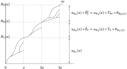
Figure 1: An example with $k_{1}=3$, $k_{2}=2$ and $k_{3}=4$.

(17), the following events coincide (see Figure 1):

$$\{\tau^{0}=+\infty,\overline{K}_{m}(x)=k\}$$

$$\qquad=\bigl{\{}u_{k_{1}}(x)<+\infty,u_{k_{2}}(x)\circ T_{x}\circ\theta_{R_{1}(x)}<+\infty,\ldots,$$

$$\hskip 38.0ptu_{k_{m}}(x)\circ T_{(m-1)x}\circ\theta_{R_{m-1}(x)}<+\infty,\tau^{0}\circ T_{mx}\circ\theta_{R_{m}(x)}=+\infty\bigr{\}}.$$

Moreover, on this event, $S_{m}(x)=R_{m}(x)$ holds. Thus

$$\mathbb{P}_{\lambda}\bigl{(}\tau^{0}=+\infty,A,t\leq S_{m}(x),\overline{K}_{m}(x)=k,\tilde{\theta}_{x}^{-m}(B)\bigr{)}$$

$$\qquad=\mathbb{P}_{\lambda}\bigl{(}A,u_{k_{1}}(x)<+\infty,u_{k_{2}}(x)\circ T_{x}\circ\theta_{R_{1}(x)}<+\infty,\ldots,$$

$$\qquad\quad\hskip 17.0ptu_{k_{m}}(x)\circ T_{(m-1)x}\circ\theta_{R_{m-1}(x)}<+\infty,t\leq R_{m}(x),$$

$$\qquad\quad\hskip 49.0pt\tau^{0}\circ T_{mx}\circ\theta_{R_{m}(x)}=+\infty,T_{mx}\circ\theta_{R_{m}(x)}\in B\bigr{)}.$$

By construction, $R_{m}(x)$ is a stopping time and the event

$$A\cap\{u_{k_{1}}(x)<+\infty\}\cap\cdots\cap\bigl{\{}u_{k_{m}}(x)\circ T_{(m-1)x}\circ\theta_{R_{m-1}(x)}<+\infty\bigr{\}}\cap\{t\leq R_{m}(x)\}$$

is measurable with respect to $\mathcal{F}_{R_{m}(x)}$. Using the strong Markov property and the spatial translation property (3), we get

$$\mathbb{P}_{\lambda}\bigl{(}\tau^{0}=+\infty,A,t\leq S_{m}(x),\overline{K}_{m}(x)=k,\tilde{\theta}_{x}^{-m}(B)\bigr{)}$$

$$\qquad=\mathbb{P}_{\lambda}\bigl{(}A,u_{k_{1}}(x)<+\infty,u_{k_{2}}(x)\circ T_{x}\circ\theta_{u_{k_{1}}(x)}<+\infty,\ldots,$$

$$\qquad\quad\hskip 33.5ptu_{k_{m}}(x)\circ T_{(m-1)x}\circ\theta_{R_{m-1}(x)}<+\infty,t\leq R_{m}(x)\bigr{)}$$

$$\qquad\quad{}\times\mathbb{P}_{{mx}.{\lambda}}(\{\tau=+\infty\}\cap B).$$

Dividing the identity by $\mathbb{P}_{\lambda}(\tau=+\infty)$, we obtain an identity of the form

$$\overline{\mathbb{P}}_{\lambda}\bigl{(}A,t\leq S_{m}(x),\tilde{\theta}_{x}^{-m}(B),\overline{K}_{m}(x)=k\bigr{)}=\psi(x,\lambda,k,m,A)\overline{\mathbb{P}}_{{mx}.{\lambda}}(B),$$

and we identify the value of $\psi(x,\lambda,k,m,A)$ by taking $B=\Omega$.

We can now state a mixing property.

Lemma 11

Let $t>0$ and $q>1$ be fixed. There exists a constant $A(t,q)$ such that for any $x\in\mathbb{Z}^{d}\setminus\{0\}$, for any $A\in\mathcal{F}_{t}$, for any $B\in\mathcal{F}$, $\lambda\in\Lambda$ and every ${\ell}\geq 1$,

$$\bigl{|}\overline{\mathbb{P}}_{\lambda}\bigl{(}A\cap(\tilde{\theta}_{x}^{\ell})^{-1}(B)\bigr{)}-\overline{\mathbb{P}}_{\lambda}(A)\overline{\mathbb{P}}_{{\ell x}.{\lambda}}(B)\bigr{|}\leq A(t,q)q^{-{\ell}}.$$

Let ${\ell}\geq 1$. With Lemma 10, we get

$$\bigl{|}\overline{\mathbb{P}}_{\lambda}\bigl{(}A\cap\tilde{\theta}_{x}^{-\ell}(B)\bigr{)}-\overline{\mathbb{P}}_{\lambda}(A)\overline{\mathbb{P}}_{\lambda}(\tilde{\theta}_{x}^{-\ell}(B))\bigr{|}$$

$$\qquad\leq\bigl{|}\overline{\mathbb{P}}_{\lambda}\bigl{(}t\leq S_{\ell}(x),A\cap\tilde{\theta}_{x}^{-\ell}(B)\bigr{)}-\overline{\mathbb{P}}_{\lambda}\bigl{(}t\leq S_{\ell}(x),A\bigr{)}\overline{\mathbb{P}}_{\lambda}(\tilde{\theta}_{x}^{-\ell}(B))\bigr{|}$$

$$\qquad\quad{}+2\overline{\mathbb{P}}_{\lambda}\bigl{(}t>S_{\ell}(x)\bigr{)}$$

$$\qquad=2\overline{\mathbb{P}}_{\lambda}\bigl{(}t>S_{\ell}(x)\bigr{)}.$$

Let us now fix $\alpha>0$.

With the Markov inequality, $\overline{\mathbb{P}}_{\lambda}(S_{\ell}(x)\leq t)\leq\exp(\alpha t)\overline{\mathbb{E}}_{\lambda}(\exp(-\alpha S_{\ell}(x)))$. Using the two last points of Corollary 9, one has

$$\overline{\mathbb{E}}_{\lambda}(\exp(-\alpha S_{\ell}(x))) \leq \overline{\mathbb{E}}_{\lambda}\Biggl{(}\exp\Biggl{(}-\alpha\sum_{j=0}^{{\ell}-1}\sigma(x)\circ\tilde{\theta}_{x}^{j}\Biggr{)}\Biggr{)}$$

$$\leq \prod_{j=0}^{{\ell}-1}\overline{\mathbb{E}}_{\lambda}\bigl{(}\exp\bigl{(}-\alpha\sigma(x)\circ\tilde{\theta}_{x}^{j}\bigr{)}\bigr{)}$$

$$= \prod_{j=0}^{{\ell}-1}\overline{\mathbb{E}}_{{jx}.{\lambda}}(\exp(-\alpha\sigma(x))).$$

Now we just have to prove the existence of some $\alpha>0$ such that for every $\lambda\in\Lambda$,

$$\overline{\mathbb{E}}_{{\lambda}}(\exp(-\alpha\sigma(x)))\leq q^{-1}.$$

Let $\rho$ be the constant given in (7):

$$\overline{\mathbb{E}}_{\lambda}(\exp(-\alpha\sigma(x))) \leq \frac{1}{\rho}\mathbb{E}_{\lambda}(\exp(-\alpha\sigma(x)))$$

$$\leq \frac{1}{\rho}\mathbb{E}_{\lambda_{\max}}(\exp(-\alpha\sigma(x)))$$

$$\leq \frac{1}{\rho}\frac{2d\lambda_{\max}}{\alpha+2d\lambda_{\max}},$$

because $\sigma(x)\geq t(x)$, and $t(x)$ stochastically dominates an exponential random variable with parameter $2d\lambda_{\max}$. This gives the desired inequality if $\alpha$ is large enough.

We can now move forward to the proof of the ergodicity properties of the systems $(\Omega,\mathcal{F},\overline{\mathbb{P}},\tilde{\theta}_{x})$. Proof of Theorem 1 We have already seen in Corollary 9 that for any $x\in\mathbb{Z}^{d}$, the probability measure $\overline{\mathbb{P}}$ is invariant under the action of $\tilde{\theta}_{x}$. To prove ergodicity, we use an embedding in a larger space to consider simultaneously a random environment and a random contact process.

We thus set $\tilde{\Omega}=\Lambda\times\Omega$, equipped with the $\sigma$-algebra $\tilde{\mathcal{F}}=\mathcal{B}(\Lambda)\otimes\mathcal{F}$, and we define a probability measure $\overline{\mathbb{Q}}$ on $\tilde{\mathcal{F}}$ by

$$\forall(A,B)\in\mathcal{B}(\Lambda)\times\mathcal{F}\qquad\overline{\mathbb{Q}}(A\times B)=\int_{\Lambda}\mathbh{1}_{A}(\lambda)\overline{\mathbb{P}}_{\lambda}(B)\,d\nu(\lambda).$$

We define the transformation $\tilde{\Theta}_{x}$ on $\tilde{\Omega}$ by setting $\tilde{\Theta}_{x}(\lambda,\omega)=(x.\lambda,\tilde{\theta}_{x}(\omega))$. It is easy to see that $\overline{\mathbb{Q}}$ is invariant under $\tilde{\Theta}_{x}$. Indeed, for $(A,B)\in\mathcal{B}(\Lambda)\times\mathcal{F}$, using Lemma 8, one has

$$\overline{\mathbb{Q}}\bigl{(}\tilde{\Theta}_{x}(\lambda,\omega)\in A\times B\bigr{)} = \overline{\mathbb{Q}}\bigl{(}x.\lambda\in A,\tilde{\theta}_{x}(\omega)\in B\bigr{)}$$

$$= \int_{\Lambda}\mathbh{1}_{A}(x.\lambda)\overline{\mathbb{P}}_{\lambda}\bigl{(}\tilde{\theta}_{x}(\omega)\in B\bigr{)}\,d\nu(\lambda)$$

$$= \int_{\Lambda}\mathbh{1}_{A}(x.\lambda)\overline{\mathbb{P}}_{x.\lambda}(B)\,d\nu(\lambda)$$

$$= \int_{\Lambda}\mathbh{1}_{A}(\lambda)\overline{\mathbb{P}}_{\lambda}(B)\,d\nu(\lambda)$$

$$= \overline{\mathbb{Q}}(A\times B).$$

Note that if $g(\lambda,\omega)=f(\lambda)$, then $\int g\,d\overline{\mathbb{Q}}=\int f\,d\nu$.

Similarly, if $g(\lambda,\omega)=f(\omega)$, then $\int g\,d\overline{\mathbb{Q}}=\int f\,d\overline{\mathbb{P}}$.

Note that $\mathcal{A}=\bigcup_{t\geq 0}\mathcal{F}_{t}$ is an algebra that generates $\mathcal{F}$. To prove that $\tilde{\theta}_{x}$ is ergodic, it is then sufficient to show that for every $A\in\mathcal{A}$,

$$\frac{1}{n}\sum_{k=0}^{n-1}\mathbh{1}_{A}(\tilde{\theta}_{x}^{k})\qquad\mbox{converges in }L^{2}(\overline{\mathbb{P}})\mbox{ to }\overline{\mathbb{P}}(A).$$ (18)

The quantity above can be seen as a function of the two variables $(\lambda,\omega)$. Thus it is equivalent to prove that the sequence of functions $(\lambda,\omega)\mapsto\frac{1}{n}\sum_{k=0}^{n-1}\mathbh{1}_{A}(\tilde{\theta}_{x}^{k}\omega)$ converges to $\overline{\mathbb{P}}(A)$ in $L^{2}(\overline{\mathbb{Q}})$. Let $A\in\mathcal{A}$ and $t>0$ be such that $A\in\mathcal{F}_{t}$. For every $(\omega,\lambda)\in\tilde{\Omega}$, we split the sum into two terms:

$$\frac{1}{n}\sum_{k=0}^{n-1}\mathbh{1}_{A}(\tilde{\theta}_{x}^{k}\omega) = \frac{1}{n}\sum_{k=0}^{n-1}\bigl{(}\mathbh{1}_{A}(\tilde{\theta}_{x}^{k}\omega)-\overline{\mathbb{P}}_{kx.\lambda}(A)\bigr{)}$$

$${}+\frac{1}{n}\sum_{k=0}^{n-1}\overline{\mathbb{P}}_{kx.\lambda}(A).$$

If we set $f(\lambda)=\overline{\mathbb{P}}_{\lambda}(A)$, the second term can be written

$$\frac{1}{n}\sum_{k=0}^{n-1}\overline{\mathbb{P}}_{kx.\lambda}(A)=\frac{1}{n}\sum_{k=0}^{n-1}f(kx.\lambda).$$

Since $x\in\operatorname{Erg}(\nu)$, the Von Neumann ergodic theorem says that this quantity converges in $L^{2}(\nu)$ to $\int fd\nu=\overline{\mathbb{P}}(A)$. Seen as a function of $(\lambda,\omega)$, it also converges in $L^{2}(\overline{\mathbb{Q}})$ to $\overline{\mathbb{P}}(A)$. Set, $k\geq 0$,

$$Y_{k}=\mathbh{1}_{A}(\tilde{\theta}_{x}^{k}\omega)-\overline{\mathbb{P}}_{\lambda}(\tilde{\theta}_{x}^{-k}(A))=\mathbh{1}_{A}(\tilde{\theta}_{x}^{k}\omega)-\overline{\mathbb{P}}_{kx.\lambda}(A)$$

and $L_{n}=Y_{0}+Y_{1}+\cdots+Y_{n-1}$. It only remains to prove that $L_{n}/n$ converges to $0$ in $L^{2}(\overline{\mathbb{Q}})$. As $Y_{k}=Y_{0}\circ\tilde{\Theta}_{x}^{k}$, the field $(Y_{k})_{k\geq 0}$ is stationary. We thus have

$$\int L_{n}^{2}\,d\overline{\mathbb{Q}} = \sum_{0\leq i,j\leq n-1}\int Y_{i}Y_{j}\,d\overline{\mathbb{Q}}$$

$$= \sum_{i=0}^{n-1}\int Y_{i}^{2}\,d\overline{\mathbb{Q}}+2\sum_{\ell=1}^{n-1}(n-\ell)\int Y_{0}Y_{\ell}\,d\overline{\mathbb{Q}}$$

$$\leq 2n\Biggl{(}\sum_{\ell=0}^{+\infty}\biggl{|}\int Y_{0}Y_{\ell}\,d\overline{\mathbb{Q}}\biggr{|}\Biggr{)}\leq 2n\Biggl{(}\sum_{\ell=0}^{+\infty}\int_{\Lambda}|\overline{\mathbb{E}}_{\lambda}(Y_{0}Y_{\ell})|\,d\nu(\lambda)\Biggr{)}$$

$$\leq 2n\Biggl{(}\sum_{\ell=0}^{+\infty}\int_{\Lambda}\bigl{|}\overline{\mathbb{P}}_{\lambda}\bigl{(}A\cap\tilde{\theta}_{x}^{-\ell}(A)\bigr{)}-\overline{\mathbb{P}}_{\lambda}(A)\overline{\mathbb{P}}_{\lambda}(\tilde{\theta}_{x}^{-\ell}(A))\bigr{|}\,d\nu(\lambda)\Biggr{)}$$

$$\leq 2n\Biggl{(}\sum_{\ell=0}^{+\infty}A(t,2)2^{-\ell}\Biggr{)}=4A(t,2)n,$$

thanks to Lemma 11. This ends the proof of (18), hence, the proof of Theorem 1.

4 Bound for the lack of subadditivity

In this section, we are going to bound quantities such as $\sigma(x+y)-[\sigma(x)+\sigma(y)\circ\tilde{\theta}_{x}]$ and $\sigma(x)-t(x)$.

We will use these results in the application of a (almost) subadditive ergodic theorem in Section 5. In both cases, we use a kind of restart argument. Considering the definition of the essential hitting time $\sigma$, we will have to deal with two types of sums of random variables that are quite different: sums of $v_{i}-u_{i}$ on one hand, and sums of $u_{i+1}-v_{i}$ on the other hand.

• The life time $v_{i}(x)-u_{i}(x)$ of the contact process starting from $x$ at time $u_{i}(x)$ can be bounded independently of the precise configuration of the process at time $u_{i}(x)$. So the control is quite simple.

• On the contrary, $u_{i+1}(x)-v_{i}(x)$, which represents the amount of time needed to reinfect site $x$ after time $v_{i}(x)$, clearly depends on the whole configuration of the process at time $v_{i}(x)$, which is not easy to control precisely and uniformly in $x$. This explains why the restart argument we use is more complex and the estimates we obtain less accurate than in more classical situations (e.g., in Section 6, we obtain the exponential estimates of Proposition 5 by standard restart arguments).

As an illustration of the first point, we easily obtain the following lemma.

Lemma 12

There exist $A,B>0$ such that for every $\lambda\in\Lambda$,

$$\forall x\in\mathbb{Z}^{d},\forall t>0\qquad\overline{\mathbb{P}}_{\lambda}\bigl{(}\exists i<K(x)\dvtx v_{i}(x)-u_{i}(x)>t\bigr{)}\leq A\exp(-Bt).$$ (19)

Let $F\dvtx\Omega\to\mathbb{R}_{+}$ be a measurable function and $x\in\mathbb{Z}^{d}$. We set

$$\mathcal{L}_{x}(F)=\sum_{i=0}^{+\infty}\mathbh{1}_{\{u_{i}(x)<+\infty\}}F\circ\theta_{u_{i}(x)}.$$

With the Markov property and the definition of $K(x)$, we have

$$\mathbb{E}_{\lambda}[\mathcal{L}_{x}(F)] = \sum_{i=0}^{+\infty}\mathbb{E}_{\lambda}\bigl{[}\mathbh{1}_{\{u_{i}(x)<+\infty\}}\bigr{]}\mathbb{E}_{\lambda}[F]=\Biggl{(}1+\sum_{i=0}^{+\infty}\mathbb{P}_{\lambda}\bigl{(}K(x)>i\bigr{)}\Biggr{)}\mathbb{E}_{\lambda}[F]$$

$$= \bigl{(}1+\mathbb{E}_{\lambda}[K(x)]\bigr{)}\mathbb{E}_{\lambda}[F]\leq\biggl{(}1+\frac{1}{\rho}\biggr{)}\mathbb{E}_{\lambda}[F],$$

where the last equality comes from Lemma 6. We choose $F=\mathbh{1}_{\{t<u_{i}(x)-v_{i}(x)<+\infty\}}$, and with estimate (7), we obtain

$$\overline{\mathbb{P}}_{\lambda}\bigl{(}\exists i<K(x)\dvtx v_{i}(x)-u_{i}(x)>t\bigr{)} \leq \frac{1}{\rho}\mathbb{P}_{\lambda}\bigl{(}\exists i<K(x)\dvtx v_{i}(x)-u_{i}(x)>t\bigr{)}$$

$$\leq \frac{1}{\rho}\mathbb{P}_{\lambda}\bigl{(}\mathcal{L}_{x}(F)\geq 1\bigr{)}\leq\frac{1}{\rho}\mathbb{E}_{\lambda}[\mathcal{L}_{x}(F)]$$

$$\leq \frac{1}{\rho}\biggl{(}1+\frac{1}{\rho}\biggr{)}\mathbb{P}_{\lambda}(t<\tau^{x}<+\infty).$$

We can then conclude with inequality (9).

To deal with the reinfection times $u_{i+1}(x)-v_{i}(x)$, the idea is to look for a point $(y,t)$ (in space–time coordinates) close to $(x,u_{i}(x))$, infected from $(0,0)$ and with infinite life time. The at-least-linear-growth estimate (10) will then ensure it does not take too long to reinfect $x$ after time $t$, just by looking at infection starting from the new source point $(y,t)$. The difficulty lies in the control of the distance between $(x,u_{i}(x))$ and a source point $(y,t)$; if the configuration around $(x,u_{i}(x))$ is “reasonable,” this point will not be too far from $(x,u_{i}(x))$, and we will obtain a good control of $u_{i+1}(x)$ and $u_{i}(x)$.

We recall that for every $x\in\mathbb{Z}^{d}$, $\omega_{x}$ is the Poisson point process giving the possible death times at site $x$, and that $M$ and $c$ are, respectively, given in (8) and (10). Note that we can assume that $M>1$. We note

$$\gamma=3M(1+1/c)>3.$$ (20)

For $x,y\in\mathbb{Z}^{d}$ and $t>0$, we say that the growth from $(y,0)$ is bad at scale $t$ with respect to $x$ if the following event occurs:

$$E^{y}(x,t) = \{\omega_{y}[0,t/2]=0\}\cup\{H^{y}_{t}\not\subset y+B_{Mt}\}\cup\{t/2<\tau^{y}<+\infty\}$$

$${}\cup\bigl{\{}\tau^{y}=+\infty,\inf\{s\geq 2t\dvtx x\in\xi^{y}_{s}\}>\gamma t\bigr{\}}.$$

We want to check that with a high probability, there is no such bad growth point in a box around $x$. So we define, for every $x\in\mathbb{Z}^{d}$, every $L>0$ and every $t>0$,

$$N_{L}(x,t)=\sum_{y\in x+B_{Mt+2}}\int_{0}^{L}\mathbh{1}_{E^{y}(x,t)}\circ\theta_{s}\,d\biggl{(}\omega_{y}+\sum_{e\in\mathbb{E}^{d}\dvtx y\in e}\omega_{e}+\delta_{0}\biggr{)}(s).$$

In other words, we count the number of points $(y,s)$ in the space–time box $(x+B_{Mt+1})\times[0,L]$ such that something happens for site $y$ at time $t$, either a possible death, or a possible infection, and at this time the bad event $E^{y}(x,t)\circ\theta_{s}$ occurs. We first check that if the space–time box has no bad points and if $u_{i}(x)$ is in the time window, then we can control the delay before the next infection.

Lemma 13

If $N_{L}(x,t)\circ\theta_{s}=0$ and $s+t\leq u_{i}(x)\leq s+L$, then $v_{i}(x)=+\infty$ or $u_{i+1}(x)-u_{i}(x)\leq\gamma t$.

By definition of $u_{i}(x)$, site $x$ is infected from $(0,0)$ at time $u_{i}(x)$. Since $s+t\leq u_{i}(x)\leq s+L$ and $u_{i}(x)$ is a possible infection time for $x$, the nonoccurrence of $E^{x}(x,t)\circ\theta_{u_{i}(x)}$ ensures that $\tau^{x}\circ\theta_{u_{i}(x)}=+\infty$ or that $\tau^{x}\circ\theta_{u_{i}(x)}\leq t/2$. If $\tau^{x}\circ\theta_{u_{i}(x)}=+\infty$, we are done because then $v_{i}(x)=+\infty$. Otherwise, note that $v_{i}(x)-u_{i}(x)\leq t/2$.

By definition, there exists an infection path $\gamma_{i}\dvtx[0,u_{i}(x)]\rightarrow\mathbb{Z}^{d}$ from $(0,0)$ to $(x,u_{i}(x))$, that is, such that $\gamma_{i}(0)=0$ and $\gamma_{i}(u_{i}(x))=x$. Consider the portion of $\gamma_{i}$ between time $u_{i}(x)-t$ and time $u_{i}(x)$. Denote by $x_{0}=\gamma_{i}(u_{i}(x)-t)$ and let us see that $x_{0}\in x+B_{Mt+2}$. Indeed, if $x_{0}\notin x+B_{Mt+2}$, we seek the first time $t_{1}$ after time $u_{i}(x)-t$ when $\gamma_{i}$ enters in $x+B_{Mt+2}$ at a site we call $x_{1}$ (note that since $x_{1}$ is in the inside boundary of $x+B_{Mt+2}$, we have $\|x-x_{1}\|_{\infty}\geq Mt+1$). Time $t_{1}$ is a possible infection time for $x_{1}$, and the nonoccurrence of $E^{x_{1}}(x,t)\circ\theta_{t_{1}}$ ensures that the infection of $x$ from $(x_{1},t_{1})$ will at least require a delay $t$, which contradicts $u_{i}(x)-t\geq 0$.

So $x_{0}\in x+B_{Mt+2}$. Since $N_{L}(x,t)\circ\theta_{s}=0$, the first possible death at site $x_{0}$ after time $u_{i}(x)-t$ cannot occur after a delay of $t/2$; thus the first time $t_{2}$ when the path $\gamma_{i}$ jumps to a different point $x_{2}$ satisfies $t_{2}\leq u_{i}(x)-t+t/2=u_{i}(x)-t/2$. Consequently, when $(x_{2},t_{2})$ infects $(x,u_{i}(x))$, it is at least $t/2$ aged, and the nonoccurrence of $E^{x_{2}}(x,t)\circ\theta_{t_{2}}$ ensures it lives forever and

$$\inf\{u\geq 2t\dvtx x\in\xi^{x_{2}}_{u}\}\circ\theta_{t_{2}}\leq\gamma t.$$

So there exists $t_{3}\in[t_{2}+2t,t_{2}+\gamma t]$ with $x\in\xi^{0}_{t_{3}}$. Since $v_{i}(x)-u_{i}(x)\leq t/2$, one has

$$t_{3}\geq t_{2}+2t\geq\bigl{(}u_{i}(x)-t\bigr{)}+2t=u_{i}(x)+t\geq v_{i}(x).$$

Finally, $u_{i+1}(x)-u_{i}(x)\leq t_{3}-u_{i}(x)\leq t_{2}-u_{i}(x)+\gamma t\leq\gamma t$.

Now we estimate the probability that a space–time box contains no bad points.

Lemma 14

There exist $A_{\mbox{{{\ref{eNL}}}}},B_{\mbox{{{\ref{eNL}}}}}>0$ such that for every $\lambda\in\Lambda$,

$$\forall L>0,\forall x\in\mathbb{Z}^{d},\forall t>0\qquad\mathbb{P}_{\lambda}\bigl{(}N_{L}(x,t)\geq 1\bigr{)}\leq A_{21}(1+L)\exp(-B_{21}t).$$ (21)

Let us first prove there exist $A,B>0$ such that for every $\lambda\in\Lambda$,

$$\quad\forall x\in\mathbb{Z}^{d},\forall t>0,\forall y\in x+B_{Mt+2}\qquad\mathbb{P}_{\lambda}(E^{y}(x,t))\leq A\exp(-Bt).$$ (22)

Let $x\in\mathbb{Z}^{d}$, $t>0$ and $y\in x+B_{Mt+2}$. If $\tau^{y}=+\infty$, there exists $z\in\xi^{y}_{2t}$ with $\tau^{z}\circ\theta_{2t}=+\infty$. Thus, definition (20) of $\gamma$ implies that

$$\bigl{\{}\tau^{y}=+\infty,\inf\{s\geq 2t\dvtx x\in\xi^{y}_{s}\}>\gamma t\bigr{\}}$$

$$\qquad\subset\{\xi^{y}_{2t}\not\subset y+B_{2Mt}\}\cup\bigcup_{z\in y+B_{2Mt}}\{t^{z}(x)\circ\theta_{2t}>(\gamma-2M)t\}$$

$$\qquad\subset\{\xi^{y}_{2t}\not\subset y+B_{2Mt}\}\cup\bigcup_{z\in y+B_{2Mt}}\biggl{\{}t^{z}(x)\circ\theta_{2t}>\frac{\|x-z\|}{c}+Mt-\frac{3}{c}\biggr{\}}.$$

Hence, with (8) and (10),

$$\mathbb{P}_{\lambda}(\tau^{y}=+\infty,\inf\{s\geq 2t\dvtx x\in\xi^{y}_{s}\}>\gamma t)$$

$$\qquad\leq A\exp(-2BMt)+(1+4Mt)^{d}A\exp\bigl{(}-B(Mt-3/c)\bigr{)}.$$

The distribution of the number $\omega_{y}([0,t/2])$ of possible deaths on site $y$ between time $0$ and time $t/2$ is a Poisson law with parameter $t/2$, so

$$\mathbb{P}_{\lambda}\bigl{(}\omega_{y}([0,t/2])=0\bigr{)}=\exp(-t/2).$$

The two remaining terms are controlled with (8) and (9); this gives (22).

Now fix $y\in x+B_{Mt+2}$ and note $\beta_{y}=\omega_{y}+\sum_{e\in\mathbb{E}^{d}\dvtx y\in e}\omega_{e}$. Under $\mathbb{P}_{\lambda}$, $\beta_{y}$ is a Poisson point process with intensity $2d\lambda_{e}$. Let $S_{0}=0$ and $(S_{n})_{n\geq 1}$ be the increasing sequence of the times given by this process:

$$\int_{0}^{L}\mathbh{1}_{E^{y}(x,t)}\circ\theta_{s}\,d(\beta_{y}+\delta_{0})(s)=\sum_{n=0}^{+\infty}\mathbh{1}_{\{S_{n}\leq L\}}\mathbh{1}_{E^{y}(x,t)}\circ\theta_{S_{n}}.$$

So, with the Markov property,

$$\mathbb{E}_{\lambda}\biggl{(}\int_{0}^{L}\mathbh{1}_{E^{y}(x,t)}\circ\theta_{s}\,d(\beta_{y}+\delta_{0})(s)\biggr{)}$$

$$\qquad=\sum_{n=0}^{+\infty}\mathbb{E}_{\lambda}\bigl{(}\mathbh{1}_{\{S_{n}\leq L\}}\mathbh{1}_{E^{y}(x,t)}\circ\theta_{S_{n}}\bigr{)}=\sum_{n=0}^{+\infty}\mathbb{E}_{\lambda}\bigl{(}\mathbh{1}_{\{S_{n}\leq L\}}\bigr{)}\mathbb{P}_{\lambda}(E^{y}(x,t))$$

$$\qquad=\bigl{(}1+\mathbb{E}_{\lambda}[\beta_{y}([0,L])]\bigr{)}\mathbb{P}_{\lambda}(E^{y}(x,t))=\bigl{(}1+L(2d\lambda_{e}+1)\bigr{)}\mathbb{P}_{\lambda}(E^{y}(x,t)).$$

So (21) follows from (22), from the remark that $\mathbb{P}_{\lambda}(N_{L}(x,t)\geq 1)\leq\mathbb{E}_{\lambda}[N_{L}(x,t)]$ and from an obvious bound on the cardinality of $B_{Mt+2}$.

Once the process is initiated, Lemma 13 can be used recursively to control $u_{i+1}(x)-u_{i}(x)$. To initiate the process, we assume that there exists a point $(u,s)$, reached from $(0,0)$, living infinitely and close to $x$ in space.

Lemma 15

For any $t,s>0$, for every $x\in\mathbb{Z}^{d}$, the following inclusion holds:

$$\{\tau^{0}=+\infty\}\cap\{\exists u\in x+B_{Mt+2},\tau_{u}\circ\theta_{s}=+\infty,u\in\xi^{0}_{s}\}$$

$$\quad{}\cap\bigl{\{}N_{K(x)\gamma t}(x,t)\circ\theta_{s}=0\bigr{\}}$$ (23)

$$\quad{}\cap\bigcap_{1\leq i<K(x)}\{v_{i}(x)-u_{i}(x)<t\}$$ (24)

$$\qquad\subset\{\tau^{0}=+\infty\}\cap\{\sigma(x)\leq s+K(x)\gamma t\}.$$ (25)

If every finite $u_{i}(x)$ is smaller than $s+t$, we are done because $\sigma(x)\leq s+t\leq s+K(x)\gamma t$. So set

$$i_{0}=\max\{i\dvtx u_{i}(x)\leq s+t\}.$$

Since $v_{i_{0}}(x)<+\infty$, the event (24) ensures that $v_{i_{0}}(x)-u_{i_{0}}(x)<t$, and so $v_{i_{0}}(x)\leq s+2t$. Now, since $\tau^{u}=+\infty$, the nonoccurrence of $E^{u}(x,t)\circ\theta_{s}$ implied by (23) says that

$$\inf\{s\geq 2t\dvtx x\in\xi^{u}_{s}\}\circ\theta_{s}\leq\gamma t,$$

which leads to $u_{i_{0}+1}(x)\leq s+\gamma t$. Noting that for any $j\geq 1$, $u_{i_{0}+j}(x+y)\geq s+{t}$, we prove by a recursive use of Lemma 13 with the event $\{N_{K(x)\gamma t}(x,t)\circ\theta_{s}=0\}$ that

$$\forall j\in\{1,\ldots,K(x)-i_{0}\}\qquad u_{i_{0}+j}\leq s+j\gamma{t}.$$

For $j=K(x)-i_{0}$, we get $\sigma(x)=u_{i_{0}+j}(x)\leq s+(K(x)-i_{0})\gamma t\leq s+K(x)\gamma t,$ which proves (25).

4.1 Bound for the lack of subadditivity

To bound $\sigma(x+y)-[\sigma(x)+\sigma(y)\circ\tilde{\theta}_{x}]$, we apply the strategy we have just explained around site $x+y$. To initiate the recursive process, one can benefit here from the existence of an infinite start at the precise point $(x+y,\sigma(x)+\sigma(y)\circ\tilde{\theta}_{y})$. Proof of Theorem 2 Let $x,y\in\mathbb{Z}^{d}$, $\lambda\in\Lambda$ and $t>0$. We set $s=\sigma(x)+\sigma(y)\circ\tilde{\theta}_{x}$:

$$\overline{\mathbb{P}}_{\lambda}\bigl{(}\sigma(x+y)>\sigma(x)+\sigma(y)\circ\tilde{\theta}_{x}+t\bigr{)}$$

$$\qquad\leq\overline{\mathbb{P}}_{\lambda}\biggl{(}K(x+y)>\frac{\sqrt{t}}{\gamma}\biggr{)}$$

$$\qquad\quad{}+\overline{\mathbb{P}}_{\lambda}\biggl{(}\tau^{0}=+\infty,K(x+y)\leq\frac{\sqrt{t}}{\gamma},\sigma(x+y)\geq s+K(x+y)\gamma\sqrt{t}\biggr{)}.$$

With the sub-geometrical behavior of the tail of $K$ given in Lemma 6 and the uniform control (7), we can control the first term. Note that if $K(x+y)\leq\frac{\sqrt{t}}{\gamma}$, then $K(x+y)\gamma\sqrt{t}\leq t$, and so that

$$\bigl{\{}N_{K(x+y)\gamma\sqrt{t}}\bigl{(}x+y,\sqrt{t}\bigr{)}\geq 1\bigr{\}}\subset\bigl{\{}N_{t}\bigl{(}x+y,\sqrt{t}\bigr{)}\geq 1\bigr{\}}.$$

We apply Lemma 15 around $x+y$, on a scale $\sqrt{t}$, an initial time $s=\sigma(x)+\sigma(y)\circ\tilde{\theta}_{x}$ and a source point $u=x+y$,

$$\overline{\mathbb{P}}_{\lambda}\biggl{(}\tau^{0}=+\infty,K(x+y)\leq\frac{\sqrt{t}}{\gamma},\sigma(x+y)\geq s+K(x+y)\gamma\sqrt{t}\biggr{)}$$

$$\qquad\leq\overline{\mathbb{P}}_{\lambda}\bigl{(}N_{t}\bigl{(}x+y,\sqrt{t}\bigr{)}\circ\theta_{s}\geq 1\bigr{)}$$ (26)

$$\qquad\quad{}+\overline{\mathbb{P}}_{\lambda}\bigl{(}\exists i<K(x+y)\dvtx v_{i}(x+y)-u_{i}(x+y)>\sqrt{t}\bigr{)}.$$

Since $N_{t}(x+y,\sqrt{t})=N_{t}(0,\sqrt{t})\circ T_{x}\circ T_{y}$ and $s=\sigma(x)+\sigma(y)\circ\tilde{\theta}_{x}$, we have

$$N_{t}\bigl{(}x+y,\sqrt{t}\bigr{)}\circ\theta_{s}=N_{t}\bigl{(}0,\sqrt{t}\bigr{)}\circ\tilde{\theta}_{y}\circ\tilde{\theta}_{x}.$$

Thus $\overline{\mathbb{P}}_{\lambda}(N_{t}(x+y,\sqrt{t})\circ\theta_{s}\geq 1)=\overline{\mathbb{P}}_{(x+y).\lambda}(N_{t}(0,\sqrt{t})\geq 1)$, which is controlled by Lemma 14 and estimate (7). Finally, (4.1) is bounded with Lemma 12.

Corollary 16

For $x,y\in\mathbb{Z}^{d}$, set $r(x,y)=(\sigma(x+y)-(\sigma(x)+\sigma(y)\circ\tilde{\theta}_{x}))^{+}$.

For any $p\geq 1$, there exists $M_{p}>0$ such that

$$\forall\lambda\in\Lambda,\forall x,y\in\mathbb{Z}^{d}\qquad\overline{\mathbb{E}}_{\lambda}[r(x,y)^{p}]\leq M_{p}.$$ (27)

We write $\overline{\mathbb{E}}_{\lambda}[r(x,y)^{p}]=\int_{0}^{+\infty}pu^{p-1}\overline{\mathbb{P}}_{\lambda}(r(x,y)>u)\,du$ and use Theorem 2.

4.2 Control of the discrepancy between hitting times and essential hitting times

To bound $\sigma(x)-t(x)$, we would like to apply the same strategy starting from $(x,t(x))$ but we do not have any natural candidate for an infinite start close to this point. We are going to look for such a point along the infection path between $(0,0)$ and $(x,t(x))$ which requires controls on a space–time box whose height (in time) of order $t(x)$, that is, of order $\|x\|$. So we will lose in the precision of the estimates and in their uniformity.

Proposition 17

There exist $A_{\mbox{{{\ref{eimportante}}}}},B_{\mbox{{{\ref{eimportante}}}}},\alpha_{\mbox{{{\ref{eimportante}}}}}>0$ such that for every $z>0$, every $x\in\mathbb{Z}^{d}$, every $\lambda\in\Lambda$,

$$\quad\overline{\mathbb{P}}_{\lambda}\bigl{(}\sigma(x)\geq t(x)+K(x)\bigl{(}\alpha_{28}\log(1+\|x\|)+z\bigr{)}\bigr{)}\leq A_{28}\exp(-B_{28}z).$$ (28)

For $x,y\in\mathbb{Z}^{d}$ and $t,L>0$, we define

$$\tilde{E}^{y}(t) = \biggl{\{}\tau_{y}<+\infty,\bigcup_{s\geq 0}H^{y}_{s}\not\subset y+B_{Mt}\biggr{\}},$$

$$\tilde{N}_{L}(x,t) = \sum_{y\in x+B_{Mt+1}}\int_{0}^{L}\mathbh{1}_{\tilde{E}^{y}(t)}\circ\theta_{s}d\biggl{(}\sum_{e\in\mathbb{E}^{d}\dvtx y\in e}\omega_{e}\biggr{)}(s).$$

With (7), (8) and (9), it is easy to get the existence of $A,B>0$ such that

$$\forall\lambda\in\Lambda,\forall x\in\mathbb{Z}^{d},\forall t>0\qquad\overline{\mathbb{P}}_{\lambda}\bigl{(}\tilde{N}_{L}(x,t)\geq 1\bigr{)}\leq A(1+L)\exp(-Bt).$$ (29)

Now, we choose the last point $(u,s)$ on the infection path between $(0,0)$ and $(x,t(x))$ such that $\tau^{u}\circ\theta_{s}=+\infty$. Note that on $\{\tau^{0}=+\infty\}$, such an $s$ always exists.

Let us see that if $\tilde{N}_{t(x)}(x,t)=0$, then $u\in x+B_{Mt+2}$. Indeed, if $\|u-x\|>Mt+2$, we consider the first point $(u^{\prime},s^{\prime})$ on the infection path after $(u,s)$ to be in $x+B_{Mt}$. The definition of $s$ ensures that the contact process starting from $(u^{\prime},s^{\prime})$ does not survive, but, since it contains $(x,t(x))$, its diameter must be larger than $Mt$, which implies that $\tilde{N}_{t(x)}(x,t)\geq 1$, and gives the desired implication.

On event $\{\tilde{N}_{t(x)}(x,t)=0\}$, we are going to apply Lemma 15 around point $(x,0)$, at scale

$$t=\frac{\alpha\log(1+\|x\|)+z}{\gamma}\geq\frac{z}{\gamma}$$

with source point $(u,s)$ and a time length $L=K(x)\gamma t$. Here and in the following, $\alpha>0$ is a large constant that will be chosen later. Since $s\leq t(x)$,

$$\overline{\mathbb{P}}_{\lambda}\bigl{(}\sigma(x)\geq t(x)+K(x)\bigl{(}\alpha\log(1+\|x\|)+z\bigr{)}\bigr{)}$$

$$\qquad=\overline{\mathbb{P}}_{\lambda}\bigl{(}\sigma(x)\geq t(x)+K(x)\gamma t\bigr{)}$$

$$\qquad\leq\overline{\mathbb{P}}_{\lambda}\bigl{(}\sigma(x)\geq s+K(x)\gamma t\bigr{)}$$

$$\qquad\leq\overline{\mathbb{P}}_{\lambda}\bigl{(}\sigma(x)\geq s+K(x)\gamma t,\tilde{N}_{t(x)}(x,t)=0\bigr{)}$$

(30)

$$\qquad\quad{}+\overline{\mathbb{P}}_{\lambda}\bigl{(}\tilde{N}_{t(x)}(x,t)\geq 1\bigr{)}$$

$$\qquad\leq\overline{\mathbb{P}}_{\lambda}\bigl{(}N_{K(x)\gamma t}(x,t)\circ\theta_{s}\geq 1\bigr{)}$$

$$\qquad\quad{}+\overline{\mathbb{P}}_{\lambda}\bigl{(}\exists i<K(x)\dvtx v_{i}(x)-u_{i}(x)>t\bigr{)}$$

$$\qquad\quad{}+\overline{\mathbb{P}}_{\lambda}\bigl{(}\tilde{N}_{t(x)}(x,t)\geq 1\bigr{)}.$$

The second term in (4.2) is bounded with Lemma 12. For the last term, we write

$$\overline{\mathbb{P}}_{\lambda}\bigl{(}\tilde{N}_{t(x)}(x,t)\geq 1\bigr{)}\leq\overline{\mathbb{P}}_{\lambda}\bigl{(}\tilde{N}_{{\|x\|}/c+z}(x,t)\geq 1\bigr{)}+\overline{\mathbb{P}}_{\lambda}\biggl{(}t(x)>\frac{\|x\|}{c}+z\biggr{)}.$$

The second term is controlled with (7) and (10), and (29) ensures that

$$\overline{\mathbb{P}}_{\lambda}\bigl{(}\tilde{N}_{{\|x\|}/c+t}(x,t)\geq 1\bigr{)} \leq A\biggl{(}1+\frac{\|x\|}{c}+z\biggr{)}\exp(-Bt)$$

$$\leq A\biggl{(}1+\frac{\|x\|}{c}+z\biggr{)}\exp\biggl{(}-\frac{B(\alpha\log(1+\|x\|)+z)}{\gamma}\biggr{)}$$

$$\leq A^{\prime}\exp(-B^{\prime}z)$$

as soon as $\alpha$ is large enough.

For the first term of (4.2), we note that $N_{K(x)\gamma t}(x,t)\circ\theta_{s}\leq N_{t(x)+K(x)\gamma t}(x,t)$. Thus

$$\overline{\mathbb{P}}_{\lambda}\bigl{(}N_{K(x)\gamma t}(x,t)\circ\theta_{s}\geq 1\bigr{)} \leq \overline{\mathbb{P}}_{\lambda}\bigl{(}N_{{\|x\|}/c+z+K(x)\gamma t}(x,t)\geq 1\bigr{)}$$

$${}+\overline{\mathbb{P}}_{\lambda}\biggl{(}t(x)\geq\frac{\|x\|}{c}+z\biggr{)}.$$

As previously stated, the second term is bounded with (7) and (10) and while using (21), we get

$$\overline{\mathbb{P}}_{\lambda}\bigl{(}N_{{\|x\|}/c+z+K(x)\gamma t}(x,t)\geq 1\bigr{)}$$

$$\qquad\leq\sum_{k=1}^{+\infty}\sqrt{\overline{\mathbb{P}}_{\lambda}\bigl{(}K(x)=k\bigr{)}}\sqrt{\overline{\mathbb{P}}_{\lambda}\bigl{(}N_{k\gamma t+{\|x\|}/c+z}(x,t)\geq 1\bigr{)}}$$

$$\qquad\leq\sum_{k=1}^{+\infty}\sqrt{\overline{\mathbb{P}}_{\lambda}\bigl{(}K(x)=k\bigr{)}}\sqrt{A_{\mbox{{{\ref{eNL}}}}}\biggl{(}k\gamma t+\frac{\|x\|}{c}+z\biggr{)}\exp(-B_{\mbox{{{\ref{eNL}}}}}t)}$$

$$\qquad\leq\sqrt{A_{\mbox{{{\ref{eNL}}}}}\biggl{(}1+\frac{\|x\|}{c}\biggr{)}(1+z)(1+\gamma t)}\exp\biggl{(}-\frac{B_{\mbox{{{\ref{eNL}}}}}}{2}t\biggr{)}$$

$$\qquad\quad{}\times\sum_{k=1}^{+\infty}\sqrt{(1+k)\overline{\mathbb{P}}_{\lambda}\bigl{(}K(x)=k\bigr{)}}.$$

The sub-geometrical behavior of the tail of $K(x)$ given by Lemma 6 ensures that the sum is finite, and we end the proof by increasing $\alpha$ if necessary.

Lemma 18

For every $p\geq 1$, there exists $C_{\mbox{{{\ref{momv}}}}}(p)>0$ such that for every $x\in\mathbb{Z}^{d}$

$$\forall\lambda\in\Lambda\qquad\overline{\mathbb{E}}_{\lambda}\bigl{(}|\sigma(x)-t(x)|^{p}\bigr{)}\leq C_{31}(p)\bigl{(}\log(1+\|x\|)\bigr{)}^{p}.\vspace*{-2pt}$$ (31)

Set $V_{x}=\frac{\sigma(x)-t(x)}{K(x)}-\alpha_{\mbox{{{\ref{eimportante}}}}}\log(1+\|x\|)$. By Proposition 17, there exists a random variable $W$ with exponential moments that stochastically dominates $V_{x}$ under $\overline{\mathbb{P}}_{\lambda}$ for every $x$ and every $\lambda$. Moreover, Lemma 6 ensures that $K(x)$ is stochastically dominated by a geometrical random variable $K^{\prime}$.

Set $v(x)=\sigma(x)-t(x)=K(x)(\alpha\log(1+\|x\|)+V_{x})$ and let $p\geq 1$. With the Minkowski inequality, we have

$$(\overline{\mathbb{E}}_{\lambda}v(x)^{p})^{1/p} \leq \alpha\log(1+\|x\|)(\overline{\mathbb{E}}_{\lambda}K(x)^{p})^{1/p}+(\overline{\mathbb{E}}_{\lambda}[K(x)^{p}V_{x}^{p}])^{1/p}$$

$$\leq \alpha\log(1+\|x\|)(\overline{\mathbb{E}}_{\lambda}K(x)^{p})^{1/p}+(\overline{\mathbb{E}}_{\lambda}K(x)^{2p}\overline{\mathbb{E}}_{\lambda}V_{x}^{2p})^{1/({2p})}$$

$$\leq \alpha\log(1+\|x\|)(\mathbb{E}K^{\prime p})^{1/p}+(\mathbb{E}K^{\prime 2p}\mathbb{E}W^{2p})^{1/({2p})},$$

and the proof is complete.

Corollary 19

$\overline{\mathbb{P}}$-a.s., $\lim_{\|x\|\to+\infty}\frac{|\sigma(x)-t(x)|}{\|x\|}=0$.

Let $p>d$. Equation (31) gives

$$\sum_{x\in\mathbb{Z}^{d}}\overline{\mathbb{E}}\frac{|\sigma(x)-t(x)|^{p}}{(1+\|x\|)^{p}}\leq C_{\mbox{{{\ref{momv}}}}}(p)\sum_{x\in\mathbb{Z}^{d}}\frac{(\log(1+\|x|))^{p}}{(1+\|x\|)^{p}}<+\infty.$$

So $(\frac{|\sigma(x)-t(x)|}{(1+\|x\|)})_{x\in\mathbb{Z}^{d}}$ is almost surely in $\ell^{p}(\mathbb{Z}^{d})$ and thus goes to $0$.

Corollary 20

There exist $A_{\mbox{{{\ref{esigmaa}}}}},B_{\mbox{{{\ref{esigmaa}}}}},C_{\mbox{{{\ref{esigmaa}}}}}>0$ such that for every $\lambda\in\Lambda$,

$$\quad\forall x\in\mathbb{Z}^{d},\forall t>0\qquad\overline{\mathbb{P}}_{\lambda}\bigl{(}\sigma(x)\geq C_{32}\|x\|+t\bigr{)}\leq A_{32}\exp\bigl{(}-B_{32}\sqrt{t}\bigr{)}.$$ (32)

Let $\alpha=\alpha_{\mbox{{{\ref{eimportante}}}}}$ be given as in Proposition 17, and note that if $K(x)\leq\frac{1}{2\alpha}\sqrt{\|x\|+t/2}$ and $z=\alpha\sqrt{\|x\|+t/2}$, then, since $\log(1+u)\leq\sqrt{u}$, we get

$$K(x)[\alpha\log(1+\|x\|)+z]\leq 2zK(x)\leq\|x\|+t/2.$$

Thus with (10) and (7),

$$\overline{\mathbb{P}}_{\lambda}\biggl{(}\sigma(x)>\biggl{(}\frac{1}{c}+1\biggr{)}\|x\|+t\biggr{)}$$

$$\qquad\leq\overline{\mathbb{P}}_{\lambda}\biggl{(}t(x)\geq\frac{\|x\|}{c}+t/2\biggr{)}+\overline{\mathbb{P}}_{\lambda}\biggl{(}K(x)>\frac{1}{2\alpha}\sqrt{\|x\|+t/2}\biggr{)}$$

$$\qquad\quad{}+\overline{\mathbb{P}}_{\lambda}\bigl{(}\sigma(x)>t(x)+K(x)\bigl{(}\alpha\log(1+\|x\|)+\alpha\sqrt{\|x\|+t/2}\bigr{)}\bigr{)}.$$

The first term is controlled with (10), the second one with Lemma 6 and the last one by Proposition 17.

Corollary 21

For any $p\geq 1$, there exists $C_{\mbox{{{\ref{moms}}}}}(p)>0$ such that

$$\forall\lambda\in\Lambda,\forall x\in\mathbb{Z}^{d}\qquad\overline{\mathbb{E}}_{\lambda}[\sigma(x)^{p}]\leq C_{33}(p)(1+\|x\|)^{p}.$$ (33)

With the Minkowski inequality, one has

$$(\overline{\mathbb{E}}_{\lambda}[\sigma(x)^{p}])^{1/p}\leq C_{\mbox{{{\ref{esigmaa}}}}}\|x\|+\bigl{(}\overline{\mathbb{E}}_{\lambda}\bigl{[}\bigl{(}\bigl{(}\sigma(x)-C_{\mbox{{{\ref{esigmaa}}}}}\|x\|\bigr{)}^{+}\bigr{)}^{p}\bigr{]}\bigr{)}^{1/p}.$$

Moreover,

$$\overline{\mathbb{E}}_{\lambda}\bigl{[}\bigl{(}\bigl{(}\sigma(x)-C_{\mbox{{{\ref{esigmaa}}}}}\|x\|\bigr{)}^{+}\bigr{)}^{p}\bigr{]}=\int_{0}^{+\infty}pu^{p-1}\overline{\mathbb{P}}_{\lambda}\bigl{(}\sigma(x)-C_{\mbox{{{\ref{esigmaa}}}}}\|x\|>u\bigr{)}\,du<+\infty$$

by Corollary 20. In classical restart arguments, the existence of exponential moments for a random variable usually comes from the following argument: if $(X_{n})_{n\in\mathbb{N}}$ are independent identically distributed random variables with exponential moments, if $K$ is independent of the $(X_{n})_{n\in\mathbb{N}}$’s and also has exponential moments, then $\sum_{0\leq n\leq K}X_{n}$ has exponential moments. Here, our difficulties to precisely bound the reinfection times $u_{i+1}-v_{i}$ prevent us to use this scheme; we thus have to use ad hoc arguments, which lead to weaker estimates.

5 Asymptotic shape theorems

We can now move forward to the proof of Theorem 3. The first step consists of proving convergence for ratios of the type $\frac{\sigma(nx)}{n}$. With Corollary 16, we know that for every $n,p\geq 0$,

$$\overline{\mathbb{E}}\bigl{[}\sigma\bigl{(}(n+p)x\bigr{)}\bigr{]}\leq\overline{\mathbb{E}}[\sigma(nx)]+\overline{\mathbb{E}}[\sigma(px)]+M_{1}.$$

Thus the Fekete lemma says that $\frac{1}{n}\overline{\mathbb{E}}[\sigma(nx)]$ has a finite limit when $n$ goes to $+\infty$ and the natural candidate for the limit of $\frac{\sigma(nx)}{n}$ is thus

$$\mu(x)=\lim_{n\to+\infty}\frac{{\overline{\mathbb{E}}}(\sigma(nx))}{n}.\vspace*{-2pt}$$

Theorem 22

$\overline{\mathbb{P}}\mbox{-a.s. }\forall x\in\mathbb{Z}^{d}\lim_{n\to+\infty}\frac{\sigma(nx)}{n}=\lim_{n\to+\infty}\frac{\overline{\mathbb{E}}\sigma(nx)}{n}=\mu(x)$.

This convergence also holds in any $L^{p}(\overline{\mathbb{P}})$, $p\geq 1$.

To prove this result, we need the two following (almost) subadditive ergodic theorems, whose proof will be given in the Appendix.

Theorem 23

Let $(\Omega,\mathcal{F},\mathbb{P})$ be a probability space, $(\theta_{n})_{n\geq 1}$ a collection of transformations leaving the probability measure $\mathbb{P}$ invariant. On this space, we consider a collection $(f_{n})_{n\geq 1}$ of integrable functions, a collection $(g_{n})_{n\geq 1}$ of nonnegative functions and a collection $(r_{n,p})_{n,p\geq 1}$ of real functions such that

$$\forall n,p\geq 1\qquad f_{n+p}\leq f_{n}+f_{p}\circ\theta_{n}+g_{p}\circ\theta_{n}+r_{n,p}.$$ (34)

We assume that:

• $c=\inf_{n\geq 1}\frac{\mathbb{E}f_{n}}{n}>-\infty$.

• $g_{1}$ is integrable, $g_{n}/n$ almost surely converges to $0$ and $\frac{\mathbb{E}g_{n}}{n}$ converges to $0$.

• There exists $\alpha>1$ and a sequence of positive numbers $(C_{p})_{p\geq 1}$ such that $\mathbb{E}[(r^{+}_{n,p})^{\alpha}]\leq C_{p}$ for every $n,p$ and

  $$\sum_{p=1}^{+\infty}\frac{C_{p}}{p^{\alpha}}<+\infty.$$

Then $\frac{1}{n}\mathbb{E}f_{n}$ converges; if $\mu$ denotes its limit, one has

$$\mathbb{E}\biggl{[}\mathop{\underline{\lim}}_{n\to+\infty}\frac{f_{n}}{n}\biggr{]}\geq\mu.$$

If we set $\underline{f}=\mathop{\underline{\lim}}_{n\to+\infty}\frac{f_{n}}{n}$, then $\underline{f}$ is invariant under the action of each $\theta_{n}$.

Theorem 24

We keep the setting and assumptions of Theorem 23. We assume, moreover, that for every $k$,

$$\frac{1}{n}\Biggl{(}f_{nk}-\sum_{i=0}^{n-1}f_{k}\circ(\theta_{k})^{i}\Biggr{)}^{+}\to 0\qquad\mbox{a.s.}$$

Then $f_{n}/n$ converges a.s. to $\underline{f}$.

Proof of Theorem 22 We apply Theorem 23 with the choices $f_{n}=\sigma(nx)$, $\theta_{n}=\tilde{\theta}_{nx}$, $g_{p}=0$, $r_{n,p}=r(nx,px)$ and the probability measure $\mathbb{P}=\overline{\mathbb{P}}$. We take $\alpha>1$. Corollary 21 gives the integrability of $\sigma(x)$ under $\overline{\mathbb{P}}$ and Corollary 16 gives the necessary controls on its moments.

We now check the extra assumption of Theorem 24; it is easy to see that

$$t(nkx)\leq\sum_{i=0}^{n-1}\sigma(kx)\circ(\tilde{\theta}_{kx})^{i},\vspace*{-2pt}$$

which implies that $(\sigma(nkx)-\sum_{i=0}^{n-1}\sigma(kx)\circ(\tilde{\theta}_{kx})^{i})^{+}\leq\sigma(nkx)-t(nkx)$.

Corollary 19 ensures that this quantity is $o(n)$. Thus $\sigma(nx)/n$ converges to a random variable $\mu(x)$, which is invariant under the action of $\tilde{\theta}_{x}$. But Theorem 1 says that this $\mu(x)$ is in fact a constant, which ends the proof of the a.s. convergence.

To prove that a sequence converges in $L^{p}$, it suffices to show that it converges a.s. and that it is bounded in $L^{q}$ for some $q>p$. Since Corollary 21 says that $f_{n}/n$ is bounded in any $L^{p}$, the proof is complete.

The next step is to prove the asymptotic shape result, namely, Theorem 3. We start by proving the shape result for the essential hitting time $\sigma$, by following the classical strategy:

• We extend $\mu$ to an asymmetric norm on $\mathbb{R}^{d}$ in Lemma 25.

• We prove that the directional convergence given by Theorem 22 is in fact uniform in the direction in Lemma 27.

• We easily deduce the shape result from this lemma in Lemma 28.

To transpose this shape result for the classical hitting time $t$ (Lemma 29), we just need to control the discrepancy between $\sigma$ and $t$; this was done in Lemma 19. Finally, the shape result for the coupled zone is proved in Lemma 30 by introducing a coupling time $t^{\prime}$ and by bounding the difference between this time $t^{\prime}$ and the essential hitting time $\sigma$.

Note that we did not succeed in proving immediately that $\mu$ could be extended to a norm, but only to an asymmetric norm; that is, the property $\mu(\lambda x)=|\lambda|\mu(x)$ a priori only holds for nonnegative $\lambda$. We will finally deduce from the asymptotic shape theorems that $\mu$ is actually a norm.

Lemma 25

The functional $\mu$ can be extended to an asymmetric norm on $\mathbb{R}^{d}$.

Homogeneity in natural integers. By extracting subsequences, we prove the homogeneity in natural integers,

$$\forall k\in\mathbb{N},\forall x\in\mathbb{Z}^{d}\qquad\mu(kx)=k\mu(x).$$

Subadditivity. One has $\sigma(nx+ny)\leq\sigma(nx)+\sigma(ny)\circ\tilde{\theta}_{nx}+r(nx,ny)$.

Since $\overline{\mathbb{P}}$ is invariant under the action of $\tilde{\theta}_{nx}$, we get, with Corollary 16,

$$\overline{\mathbb{E}}\sigma(nx+ny)\leq\overline{\mathbb{E}}\sigma(nx)+\overline{\mathbb{E}}\sigma(ny)+\overline{\mathbb{E}}r(nx,ny)\leq\overline{\mathbb{E}}\sigma(nx)+\overline{\mathbb{E}}\sigma(ny)+M_{1}.$$

We deduce that $\forall x\in\mathbb{Z}^{d},\forall y\in\mathbb{Z}^{d},\mu(x+y)\leq\mu(x)+\mu(y)$.

Extension to $\mathbb{R}^{d}$. The Fekete lemma ensures that

$$\mu(x)+M_{1}=\inf_{n\geq 1}\frac{\overline{\mathbb{E}}{\sigma(nx)+M_{1}}}{n},$$

so $\mu(x)\leq\overline{\mathbb{E}}\sigma(x)$. Corollary 21 gives some $L>0$ such that $\overline{\mathbb{E}}\sigma(x)\leq L\|x\|$ for any $x$. Finally, $\mu(x)\leq L\|x\|$ for every $x\in\mathbb{Z}^{d}$, which leads to $|\mu(x)-\mu(y)|\leq L\|x-y\|$. We can then extend $\mu$ to $\mathbb{Q}^{d}$ par homogeneity, then to $\mathbb{R}^{d}$ by uniform continuity.

Positivity. Let $M$ be given by Proposition 5. With (8), we obtain

$$\overline{\mathbb{P}}\biggl{(}\sigma(nx)<\frac{n\|x\|}{2M}\biggr{)} \leq \overline{\mathbb{P}}\biggl{(}t(nx)<\frac{n\|x\|}{2M}\biggr{)}\leq\overline{\mathbb{P}}\bigl{(}\xi_{{n\|x\|}/{M}}\not\subset B_{{n\|x\|}/2}\bigr{)}$$

$$\leq \int\frac{\mathbb{P}_{\lambda}(\tau^{0}=+\infty,\xi^{0}_{{n\|x\|}/({2M})}\not\subset B_{{n\|x\|}/2})}{\mathbb{P}_{\lambda}(\tau^{0}=+\infty)}\,d\nu(\lambda)$$

$$\leq \frac{A}{\rho}\exp\biggl{(}-B\frac{n\|x\|}{2M}\biggr{)}.$$

With the Borel–Cantelli lemma, we deduce that $\mu(x)\geq\frac{1}{2M}\|x\|$. This inequality, once established for every $x\in\mathbb{Z}^{d}$, can be extended by homogeneity and continuity to $\mathbb{R}^{d}$. So $\mu$ is an asymmetric norm.

In the following, we set $C=2C_{\mbox{{{\ref{esigmaa}}}}}$, where $C_{\mbox{{{\ref{esigmaa}}}}}$ is as given in Corollary 20.

Lemma 26

For every $\varepsilon>0$, $\overline{\mathbb{P}}$-a.s., there exists $R>0$ such that

$$\forall x,y\in\mathbb{Z}^{d}\qquad(\|x\|\geq R\mbox{ and }\|x-y\|\leq\varepsilon\|x\|)\Longrightarrow\bigl{(}|\sigma(x)-\sigma(y)|\leq C\varepsilon\|x\|\bigr{)}.$$

For $m\in\mathbb{N}$ and $\varepsilon>0$, we define the event

$$A_{m}(\varepsilon)=\{\exists x,y\in\mathbb{Z}^{d}\dvtx\|x\|=m,\|x-y\|\leq\varepsilon m\mbox{ and }|\sigma(x)-\sigma(y)|>C\varepsilon m\}.$$

Noting that

$$A_{m}(\varepsilon)\subset\mathop{\bigcup_{(1-\varepsilon)m\leq\|x\|\leq(1+\varepsilon)m}}_{\|x-y\|\leq\varepsilon m}\{\sigma(y-x)\circ\tilde{\theta}_{x}+r(x,y-x)>C\varepsilon m\},$$

we see, with Corollaries 20 and 16, that

$$\overline{\mathbb{P}}_{\lambda}(A_{m}(\varepsilon)) \leq \mathop{\sum_{(1-\varepsilon)m\leq\|x\|\leq(1+\varepsilon)m}}_{\|z\|\leq\varepsilon m}\overline{\mathbb{P}}_{{\lambda}}\bigl{(}\sigma(z)\circ\tilde{\theta}_{x}+r(x,z)>C\varepsilon m\bigr{)}$$

$$\leq \mathop{\sum_{(1-\varepsilon)m\leq\|x\|\leq(1+\varepsilon)m}}_{\|z\|\leq\varepsilon m}\overline{\mathbb{P}}_{{x}.{\lambda}}\bigl{(}\sigma(z)>2C\varepsilon m/3\bigr{)}$$

$${}+\overline{\mathbb{P}}_{{\lambda}}\bigl{(}r(x,y-x)>C\varepsilon m/3\bigr{)}$$

$$\leq (1+2\varepsilon m)^{d}\bigl{(}1+2(1+\varepsilon)m\bigr{)}^{d}A_{\mbox{{{\ref{esigmaa}}}}}\exp\bigl{(}-B_{\mbox{{{\ref{esigmaa}}}}}\sqrt{C\varepsilon m/3}\bigr{)}$$

$${}+A_{\mbox{{{\ref{momecart}}}}}\exp\bigl{(}-B_{\mbox{{{\ref{momecart}}}}}\sqrt{C^{\prime}\varepsilon m/3}\bigr{)}$$

by Corollary 20 and Theorem 2. Integrating then with respect to $\lambda$, we conclude the proof with the Borel–Cantelli lemma.

Lemma 27

$\overline{\mathbb{P}}$-a.s. $\lim_{\|x\|\to+\infty}\frac{|\sigma(x)-\mu(x)|}{\|x\|}=0$.

Assume by contradiction that there exists $\varepsilon>0$ such that the event “$|\sigma(x)-\mu(x)|>\varepsilon\|x\|$ for infinitely many values of $x$” has a positive probability. We focus on this event. There exists a random sequence $(y_{n})_{n\geq 0}$ of sites in $\mathbb{Z}^{d}$ such that $\|y_{n}\|_{1}\rightarrow+\infty$ and, for every $n$, $|\sigma(y_{n})-\mu(y_{n})|\geq\varepsilon\|y_{n}\|_{1}$. By extracting a subsequence, we can assume that

$$\frac{y_{n}}{\|y_{n}\|_{1}}\rightarrow z.$$

Fix $\varepsilon_{1}>0$ (to be chosen later); we can find $z^{\prime}\in\operatorname{Erg}(\nu)$ such that

$$\biggl{\|}\frac{z^{\prime}}{\|z^{\prime}\|_{1}}-z\biggr{\|}_{1}\leq\varepsilon_{1}.$$

For each $y_{n}$, we can find an integer point on $\mathbb{R}z^{\prime}$ close to $y_{n}$. Let $h_{n}$ be the integer part of $\frac{\|y_{n}\|_{1}}{\|z^{\prime}\|_{1}}$. We have

$$\|y_{n}-h_{n}.z^{\prime}\|_{1} \leq \biggl{\|}y_{n}-\frac{\|y_{n}\|_{1}}{\|z^{\prime}\|_{1}}z^{\prime}\biggr{\|}_{1}+\biggl{|}\frac{\|y_{n}\|_{1}}{\|z^{\prime}\|_{1}}-h_{n}\biggr{|}\|z^{\prime}\|_{1}$$

$$\leq \|y_{n}\|_{1}\biggl{\|}\frac{y_{n}}{\|y_{n}\|_{1}}-\frac{z^{\prime}}{\|z^{\prime}\|_{1}}\biggr{\|}_{1}+\|z^{\prime}\|_{1}.$$

Take $N>0$ large enough to have $(n\geq N)\Rightarrow(\|\frac{y_{n}}{\|y_{n}\|_{1}}-z\|_{1}\leq\varepsilon_{1})$. By our choice for $z^{\prime}$, one has

$$(n\geq N)\Rightarrow\biggl{(}\biggl{\|}\frac{y_{n}}{\|y_{n}\|_{1}}-\frac{z^{\prime}}{\|z^{\prime}\|_{1}}\biggr{\|}_{1}\leq 2\varepsilon_{1}\biggr{)}$$

and, consequently, $\|y_{n}-h_{n}.z^{\prime}\|_{1}\leq 2\varepsilon_{1}\|y_{n}\|_{1}+\|z^{\prime}\|_{1}$. Thus, increasing $N$ if necessary, one has, for every $n\geq N$, $\|y_{n}-h_{n}.z^{\prime}\|_{1}\leq 3\varepsilon_{1}\|y_{n}\|_{1}$. But if $N$ is large enough, Lemma 26 ensures that

$$\forall n\geq N\qquad|\sigma(y_{n})-\sigma(h_{n}.z^{\prime})|\leq 3C\varepsilon_{1}\|y_{n}\|_{1}.$$

Finally, for every large $n$, we have

$$|\sigma(y_{n})-\mu(y_{n})|$$

$$\qquad\leq|\sigma(y_{n})-\sigma(h_{n}.z^{\prime})|+|\sigma(h_{n}.z^{\prime})-\mu(h_{n}.z^{\prime})|+|\mu(h_{n}.z^{\prime})-\mu(y_{n})|$$

$$\qquad\leq 3C\varepsilon_{1}\|y_{n}\|_{1}+h_{n}\biggl{|}\frac{\sigma(h_{n}.z^{\prime})}{h_{n}}-\mu(z^{\prime})\biggr{|}+L\|h_{n}.z^{\prime}-y_{n}\|_{1}$$

$$\qquad\leq 3C\varepsilon_{1}\|y_{n}\|_{1}+(1+\varepsilon_{1})\frac{\|y_{n}\|_{1}}{\|z^{\prime}\|_{1}}\biggl{|}\frac{\sigma(h_{n}.z^{\prime})}{h_{n}}-\mu(z^{\prime})\biggr{|}+3\varepsilon_{1}L\|y_{n}\|_{1}.$$

But the a.s. convergence in the $z^{\prime}$ direction ensures that for every large $n$,

$$\biggl{|}\frac{\sigma(h_{n}.z^{\prime})}{h_{n}}-\mu(z^{\prime})\biggr{|}\leq\varepsilon_{1}.$$

Now if $\varepsilon_{1}>0$ is small, we obtain, for every large $n$, $|\sigma(y_{n})-\mu(y_{n})|<\varepsilon\|y_{n}\|_{1};$ this brings contradiction and the proof is complete.

We can now prove the shape result for the “fattened” version $\tilde{G}_{t}$ of $G_{t}=\{x\in\mathbb{Z}^{d}\dvtx\sigma(x)\leq t\}$; we recall that $A_{\mu}$ is the unit ball for $\mu$.

Lemma 28

For every $\varepsilon>0$, $\overline{\mathbb{P}}$-a.s., for every large $t$,

$$(1-\varepsilon)A_{\mu}\subset\frac{\tilde{G}_{t}}{t}\subset(1+\varepsilon)A_{\mu}.\vspace*{-3pt}$$

Let us prove by contradiction that if $t$ is large enough, $\frac{G_{t}}{t}\subset(1+\varepsilon)A_{\mu}$. Thus assume that there exists an increasing sequence$(t_{n})_{n\geq 1}$, with $t_{n}\to+\infty$ and $\frac{G_{t_{n}}}{t_{n}}\not\subset(1+\varepsilon)A_{\mu}$; so there exists $x_{n}$ with $\sigma(x_{n})\leq t_{n}$ and $\mu(x_{n})/t_{n}>1+\varepsilon$. So $\mu(x_{n})/\sigma(x_{n})>1+\varepsilon$, which contradicts the uniform convergence of Lemma 27. Since $\mu(x_{n})>t_{n}(1+\varepsilon)$, the sequence $(\|x_{n}\|)_{n\geq 1}$ goes to infinity.

For the inverse inclusion, we still assume by contradiction that there exists an increasing sequence $(t_{n})_{n\geq 1}$, with $t_{n}\to+\infty$ and $(1-\varepsilon)A_{\mu}\not\subset\frac{\tilde{G}_{t_{n}}}{t_{n}}$; this means we can find $x_{n}$ with $\mu(x_{n})\leq(1-\varepsilon)t_{n}$, but $\sigma(x_{n})>t_{n}$. Since $t_{n}$ goes to $+\infty$, the sequence $(x_{n})_{n\geq 1}$ is not bounded and satisfies $\frac{\mu(x_{n})}{\sigma(x_{n})}<1-\varepsilon$; this contradicts once again the uniform convergence of Lemma 27 and the proof is complete.

Then we immediately recover the uniform convergence result for the hitting time $t$ via Lemma 19, and, by an argument similar to the one used in Lemma 28, the asymptotic shape result for the “fattened” version $\tilde{H}_{t}$ of $H_{t}=\{x\in\mathbb{Z}^{d}\dvtx t(x)\leq t\}$.

Lemma 29

$\overline{\mathbb{P}}$-a.s., $\lim_{\|x\|\to+\infty}\frac{t(x)-\mu(x)}{\|x\|}=0$, and for every $\varepsilon>0$, $\overline{\mathbb{P}}$-a.s., for every large $t$, $(1-\varepsilon)A_{\mu}\subset\frac{\tilde{H}_{t}}{t}\subset(1+\varepsilon)A_{\mu}$.

It only remains now to prove the shape result for the coupled zone $\tilde{K}^{\prime}_{t}$, which is the “fattened” version of $K^{\prime}_{t}=\{x\in\mathbb{Z}^{d}\dvtx\forall s\geq t\xi^{0}_{s}(x)=\xi^{\mathbb{Z}^{d}}_{s}(x)\}$.

Lemma 30

For every $\varepsilon>0$, $\overline{\mathbb{P}}$-a.s., for every large $t$, $(1-\varepsilon)A_{\mu}\subset\frac{\tilde{K}^{\prime}_{t}\cap\tilde{G}_{t}}{t}$.

Since $t\mapsto K^{\prime}_{t}\cap G_{t}$ is nondecreasing, we use the same scheme of proof as for Lemma 28. We set, for $x\in\mathbb{Z}^{d}$,

$$t^{\prime}(x)=\inf\{t\geq 0\dvtx x\in K^{\prime}_{t}\cap G_{t}\}.$$

It is then sufficient to prove that $\overline{\mathbb{P}}$-a.s., $\lim_{\|x\|\to+\infty}\frac{|t^{\prime}(x)-\sigma(x)|}{\|x\|}=0$.

By definition, $t^{\prime}(x)\geq\sigma(x)$; thus it is sufficient to prove the existence of constants $A^{\prime},B^{\prime}>0$ such that

$$\forall x\in\mathbb{Z}^{d},\forall s\geq 0\qquad\overline{\mathbb{P}}\bigl{(}t^{\prime}(x)-\sigma(x)\geq s\bigr{)}\leq A^{\prime}e^{-B^{\prime}s}.$$ (35)

$\bullet$ First note that for every $t\geq 0$, $K_{\sigma(x)+t}\supset x+K_{t}\circ\tilde{\theta}_{x}$.

Indeed, let $z\in x+K_{t}\circ\tilde{\theta}_{x}$. First consider the case $z\notin\xi_{\sigma(x)+t}^{\mathbb{Z}^{d}}$. Since, by additivity (2.3), $\xi_{\sigma(x)+t}^{0}\subset\xi_{\sigma(x)+t}^{\mathbb{Z}^{d}}$, we have $z\notin\xi_{\sigma(x)+t}^{0}$, and so that $z\in K_{\sigma(x)+t}$.

Consider now the case $z\in\xi^{\mathbb{Z}^{d}}_{\sigma(x)+t}$. Since, by additivity, $\xi^{\mathbb{Z}^{d}}_{\sigma(x)}\subset\xi^{\mathbb{Z}^{d}}_{0}\circ\tilde{\theta}_{x}$, we have $y=z-x\in\xi^{\mathbb{Z}^{d}}_{t}\circ\tilde{\theta}_{x}$. But since $y\in K_{t}\circ\tilde{\theta}_{x}$, the definition of $K_{t}$ implies that $\xi^{0}_{t}(y)\circ\tilde{\theta}_{x}=\xi^{\mathbb{Z}^{d}}_{t}(y)\circ\tilde{\theta}_{x}=1$. Since $x\in\xi^{0}_{\sigma(x)}$ and $y\in\xi^{0}_{t}\circ\tilde{\theta}_{x}$, we obtain $z=x+y\in\xi^{0}_{\sigma(x)+t}$, and so $z\in K_{\sigma(x)+t}$.

$\bullet$ Fix $s\geq 0$. The previous point says that

$$\biggl{(}\bigcap_{t\geq s}K_{\sigma(x)+t}\biggr{)}\supset\biggl{(}x+\bigcap_{t\geq s}(K_{t}\circ\tilde{\theta}_{x})\biggr{)}\quad\mbox{and so}\quad K^{\prime}_{\sigma(x)+s}\supset\bigl{(}x+(K^{\prime}_{s}\circ\tilde{\theta}_{x})\bigr{)}.$$

Since $\overline{\mathbb{P}}$ is invariant under $\tilde{\theta}_{x}$, we get

$$\overline{\mathbb{P}}\bigl{(}t^{\prime}(x)>\sigma(x)+s\bigr{)} = \overline{\mathbb{P}}\bigl{(}x\notin K^{\prime}_{\sigma(x)+s}\cap G_{\sigma(x)+s}\bigr{)}$$

$$= \overline{\mathbb{P}}\bigl{(}x\notin K^{\prime}_{\sigma(x)+s}\bigr{)}\leq\overline{\mathbb{P}}\bigl{(}x\notin(x+K^{\prime}_{s}\circ\tilde{\theta}_{x})\bigr{)}$$

$$\leq \overline{\mathbb{P}}(0\notin K^{\prime}_{s}\circ\tilde{\theta}_{x})=\overline{\mathbb{P}}(0\notin K^{\prime}_{s}).$$

We conclude with (11).

Let us finally prove that $\mu$ is a norm. Considering Lemma 25, we only have to prove that $\mu(x)=\mu(-x)$ holds for each $x\in\mathbb{Z}^{d}$. This would be immediate if we had supposed that the law $\nu$ of the random environment was invariant under the central symmetry. But, in general, we have to use a time reversal argument and the shape theorem for the coupled zone. We first give a characterization of $\mu$ that will allow us to use the symmetries of the model.

Lemma 31

Let us define $\check{\mathbb{P}}$ by $\check{\mathbb{P}}(A)=\int_{\Lambda}\mathbb{P}_{\lambda}(A)\,d\nu(\lambda)$. Then, for each $x\in\mathbb{Z}^{d}$

$$\mu(x)=\sup\Bigl{\{}a>0;\mathop{\underline{\lim}}_{n\to+\infty}\check{\mathbb{P}}(nx\in\xi_{n/a})>0\Bigr{\}}.$$

Define $g(x)=\sup\{a>0;\mathop{\underline{\lim}}_{n\to+\infty}\check{\mathbb{P}}(nx\in\xi_{n/a})>0\}$. Let $a>\mu(x)$. By the asymptotic shape theorem, $\lim_{n\to+\infty}\mathbb{P}_{\lambda}(nx\in\xi_{n/a})=0$ $\nu$ almost surely holds, so by dominated convergence, $\lim_{n\to+\infty}\check{\mathbb{P}}(nx\in\xi_{n/a})=0$. This gives $g(x)\leq\mu(x)$. Now take some $a<\mu(x)$. We will show that

$$\mathop{\underline{\lim}}_{n\to+\infty}{\mathbb{P}}_{\lambda}(nx\in\xi_{n/a})\geq\mathbb{P}_{\lambda_{\min}}(\tau=+\infty)^{2},\qquad\nu\mbox{-a.s.},$$

which will give

$$\mathop{\underline{\lim}}_{n\to+\infty}\check{\mathbb{P}}(nx\in\xi_{n/a})\geq\int_{\Lambda}\mathop{\underline{\lim}}_{n\to+\infty}{\mathbb{P}}_{\lambda}(nx\in\xi_{n/a})\,d\nu\geq\mathbb{P}_{\lambda_{\min}}(\tau=+\infty)^{2}$$

by Fatou’s lemma, whence $g(x)\geq a$, which will lead to $g(x)=\mu(x)$. Obviously, $\mathop{\underline{\lim}}_{n\to+\infty}{\mathbb{P}}_{\lambda}(nx\in\xi_{n/a})\geq\mathop{\underline{\lim}}_{n\to+\infty}{\mathbb{P}}_{\lambda}(nx\in\xi_{n/a},\tau^{0}=+\infty)$. However, the convergence theorem for the coupled zone implies that

$$\lim_{n\to+\infty}\mathbb{P}_{\lambda}(nx\in\xi^{\mathbb{Z}^{d}}_{n/a},nx\notin\xi_{n/a},\tau^{0}=+\infty)=0,\qquad\nu\mbox{-a.s.},$$

hence, by a classical time-reversal argument and using the FKG inequality,

$$\mathop{\underline{\lim}}_{n\to+\infty}{\mathbb{P}}_{\lambda}(nx\in\xi_{n/a}) \geq \mathop{\underline{\lim}}_{n\to+\infty}\mathbb{P}_{\lambda}(nx\in\xi^{\mathbb{Z}^{d}}_{n/a},\tau^{0}=+\infty)$$

$$\geq \mathop{\underline{\lim}}_{n\to+\infty}\mathbb{P}_{\lambda}(nx\in\xi^{\mathbb{Z}^{d}}_{n/a})\mathbb{P}_{\lambda}(\tau^{0}=+\infty)$$

$$\geq \mathop{\underline{\lim}}_{n\to+\infty}\mathbb{P}_{\lambda}\biggl{(}\tau^{nx}\geq\frac{n}{a}\biggr{)}\mathbb{P}_{\lambda}(\tau^{0}=+\infty)$$

$$\geq \mathbb{P}_{\lambda_{\min}}(\tau=+\infty)^{2},$$

which ends the proof of the lemma.

We now have a handsome expression to prove the symmetry property. Actually, for every $x\in\mathbb{Z}^{d},t>0,\lambda\in\Lambda$, a time-reversal argument proves that $\mathbb{P}_{\lambda}(x\in\xi_{t})=\mathbb{P}_{x.\lambda}(-x\in\xi_{t})$, hence integrating with respect to $\nu$ and using the invariance of $\nu$ under the translation by $x$,

$$\check{\mathbb{P}}(x\in\xi_{t})=\check{\mathbb{P}}(-x\in\xi_{t}),$$

which, with Lemma 31, gives the symmetry of $\mu$.

6 Uniform controls of the growth

The aim of this section is to establish some of the uniform controls announced in Proposition 5. To control the growth of the contact process, we need some lemmas on the Richardson model.

6.1 Some lemmas on the Richardson model

We call Richardson model with parameter $\lambda$ the time-homogeneous, $\mathcal{P}(\mathbb{Z}^{d})$-valued Markov process$(\eta_{t})_{t\geq 0}$, whose evolution is defined as follows: an empty site $z$ becomes infected at rate $\lambda\sum_{\|z-z^{\prime}\|_{1}=1}\eta_{t}(z^{\prime})$, the different evolutions being independent. Thanks to the graphical construction, we can, for each $\lambda\in\Lambda$, build a coupling of the contact process in environment $\lambda$ with the Richardson model with parameter $\lambda_{\max}$, in the following way: at any time $t$, the space occupied by the contact process is contained in the space occupied by the Richardson model.

The first lemma, whose proof is omitted, easily follows from the representation of the Richardson model in terms of first passage percolation, together with a path counting argument.

Lemma 32

For every $\lambda>0$, there exist constants $A,B>0$ such that

$$\forall t\geq 0\qquad\mathbb{P}(\eta_{1}\not\subset B_{t})\leq A\exp(-Bt).\vspace*{-3pt}$$

Lemma 33

For every $\lambda>0$, there exist constants $A,B,M>0$ such that

$$\forall s\geq 0\qquad\mathbb{P}(\exists t\geq 0\dvtx\eta_{t}\not\subset B_{Mt+s})\leq A\exp(-Bs).\vspace*{-3pt}$$

The representation of the Richardson model in terms of first passage percolation ensures the existence of $A^{\prime},B^{\prime},M^{\prime}>0$ such that for each $t\geq 0$,

$$\mathbb{P}(\eta_{t}\not\subset B_{M^{\prime}t})\leq A^{\prime}\exp(-B^{\prime}t).$$ (36)

For more details, one can refer to Kesten kesten .

We first control the process in integer times thanks to the following estimate:

$$\mathbb{P}(\exists k\in\mathbb{N}\dvtx\eta_{k}\not\subset B_{M^{\prime}k+s/2}) \leq \mathbb{P}\bigl{(}\exists k\in\mathbb{N}\dvtx\eta_{k+s/(2M^{\prime})}\not\subset B_{M^{\prime}k+s/2}\bigr{)}$$

$${\leq} \sum_{k=0}^{+\infty}\mathbb{P}\bigl{(}\eta_{k+s/(2M^{\prime})}\not\subset B_{M^{\prime}k+s/2}\bigr{)}$$

$$\leq \frac{A^{\prime}}{1-\exp(-B^{\prime})}\exp\biggl{(}-\frac{B^{\prime}s}{2M^{\prime}}\biggr{)}.$$

Let us now control the fluctuations between integer times. Let $M>M^{\prime}$,

$$\mathbb{P}(\{\exists t\geq 0\dvtx\eta_{t}\not\subset B_{Mt+s}\}\cap\{\forall k\in\mathbb{N},\eta_{k}\subset B_{M^{\prime}k+s/2}\})$$

(38)

$$\qquad\leq\sum_{k=0}^{+\infty}\mathbb{P}(\exists t\in[k,k+1]\dvtx\eta_{k}\subset B_{M^{\prime}k+s/2}\mbox{ and }\eta_{t}\not\subset B_{Mt+s}).$$

Then, denoting by $C^{\prime}>0$ a constant such that $|B_{t}|\leq C^{\prime}(1+t)^{d}$ and by $A,B$ the constants appearing in Lemma 32,

$$\mathbb{P}(\exists t\in[k,k+1]\dvtx\eta_{k}\subset B_{M^{\prime}k+s/2}\mbox{ and }\eta_{t}\not\subset B_{Mt+s})$$

$$\qquad\leq\mathbb{P}(\eta_{k}\subset B_{M^{\prime}k+s/2}\mbox{ and }\eta_{k+1}\not\subset B_{Mk+s})$$

$$\qquad\leq|B_{M^{\prime}k+s/2}|\mathbb{P}\bigl{(}\eta_{1}\not\subset B_{k(M-M^{\prime})+s/2}\bigr{)}$$ (39)

$$\qquad\leq C^{\prime}(1+M^{\prime}k+s/2)^{d}A\exp\bigl{(}-B\bigl{(}k(M-M^{\prime})+s/2\bigr{)}\bigr{)}$$

$$\qquad\leq AC^{\prime}(1+s/2)^{d}\exp(-Bs/2)(1+M^{\prime}k)^{d}\exp\bigl{(}-B\bigl{(}k(M-M^{\prime})\bigr{)}\bigr{)}.$$

Inequality (6.1) comes from the Markov property and from the subadditivity of the contact process. Since the series $((1+M^{\prime}k)^{d}\exp(-B(k(M-M^{\prime})))_{k\geq 1}$ converges, the desired result follows from (6.1) and (6.1).

6.2 A restart procedure

We will use here a so-called restart argument, which can be summed up as follows. We couple the system that we want to study (the strong system) with a system that it stochastically dominates (the weak system), and that is best understood. Then, we can transport some of the properties of the known system to the one we study; we let the processes simultaneously evolve and, each time the weaker dies and the stronger remains alive, we restart a copy of the weakest, coupled with the strongest again. Thus, either both processes die before we found any weak process surviving. In this case, the control of large finite lifetimes for the weak can be transposed to the strongest one, or the strongest indefinitely survives and is finally coupled with a weak surviving one. In that case, a bound for the time that is necessary to find a successful restart permits us to transfer properties of the weak surviving process to the strong one.

This technique is already old; that can be found, for example, in Durrett MR757768 , Section 12, in a very pure form. It is also used by Durrett and Griffeath MR656515 , in order to transfer some controls for the one-dimensional contact process to the contact process in a larger dimension. We will use it here by coupling the contact process in inhomogeneous environment $\lambda\in\Lambda$ with the contact process with a constant birth rate $\lambda_{\min}$. Here, the assumption $\lambda_{\min}>\lambda_{c}(\mathbb{Z}^{d})$ matters.

To this end, we will couple collections of Poisson point processes. Fix $\lambda\in\Lambda$. We can build a probability measure $\tilde{\mathbb{P}}_{\lambda}$ on $\Omega\times\Omega$ under which:

• the first coordinate $\omega$ is a collection $((\omega_{e})_{e\in\mathbb{E}^{d}},(\omega_{z})_{z\in\mathbb{Z}^{d}})$ of Poisson point processes, with respective intensities $(\lambda_{e})_{e\in\mathbb{E}^{d}}$ for the bond-indexed processes, and intensity $1$ for the site-indexed processes.

• the second coordinate $\eta$ is a collection $((\eta_{e})_{e\in\mathbb{E}^{d}},(\eta_{z})_{z\in\mathbb{Z}^{d}})$ of Poisson point processes, with intensity $\lambda_{\min}$ for the bond-indexed processes, and intensity $1$ for the site-indexed processes.

• site-indexed Poisson point processed (death times) coincide; for every $z\in\mathbb{Z}^{d}$, $\eta_{z}=\omega_{z}$.

• bond-indexed Poisson point processed (birth-times candidates) are coupled; for each $e\in\mathbb{E}^{d}$, the support of $\eta_{e}$ is included in the support of $\omega_{e}$.

We denote by $\xi^{A}=\xi^{A}(\omega,\eta)$ the contact process in environment $\lambda$ starting from $A$ and built from the Poisson process collection $\omega$, and $\zeta^{B}=\zeta^{B}(\omega,\eta)$ the contact process in environment $\lambda_{\min}$ starting from $B$ and built from the Poisson process collection $\eta$. If $B\subset A$, then $\tilde{\mathbb{P}}_{\lambda}$ almost surely, $\zeta_{t}^{B}\subset\xi_{t}^{A}$ holds for each $t\geq 0$. We can note that the process $(\xi^{A},\zeta^{B})$ is a Markov process.

We introduce the lifetimes of both processes:

$$\tau=\inf\{t\geq 0\dvtx\xi^{0}_{t}=\varnothing\}\quad\mbox{and}\quad\mbox{for }x\in\mathbb{Z}^{d}\qquad\tau^{\prime}_{x}=\inf\{t\geq 0\dvtx\zeta^{x}_{t}=\varnothing\}.$$

Note that the law of $\tau^{\prime}_{x}$ under $\tilde{\mathbb{P}}_{\lambda}$ is the law of $\tau_{x}$ under $\mathbb{P}_{\lambda_{\min}}$; it actually does not depend on the process starting point, because the model with constant birth rate is translation invariant.

We recursively define a sequence of stopping times $(u_{k})_{k\geq 0}$ and a sequence of points $(z_{k})_{k\geq 0}$, letting $u_{0}=0$, $z_{0}=0$ and for each $k\geq 0$:

• if $u_{k}<+\infty$ and $\xi_{u_{k}}\neq\varnothing$, then $u_{k+1}=\tau^{\prime}_{z_{k}}\circ\theta_{u_{k}}$;

• if $u_{k}=+\infty$ or if $\xi_{u_{k}}=\varnothing$, then $u_{k+1}=+\infty$;

• if $u_{k+1}<+\infty$ and $\xi_{u_{k+1}}\neq\varnothing$, then $z_{k+1}$ is the smallest point of $\xi_{u_{k+1}}$ for the lexicographic order;

• if $u_{k+1}=+\infty$ or if $\xi_{u_{k+1}}=\varnothing$, then $z_{k+1}=+\infty$.

In other words, until $u_{k}<+\infty$ and $\xi_{u_{k}}\neq\varnothing$, we take in $\xi_{u_{k}}$ the smallest point $z_{k}$ for the lexicographic order, and look at the lifetime of the weakest process, namely, $\zeta$, starting from $z_{k}$ at time $u_{k}$. The restart procedure can stop in two ways; either we find $k$ such that $u_{k}<+\infty$ and $\xi_{u_{k}}=\varnothing$, which implies that the strongest process (which contains the weak) precisely dies at time $u_{k}$, or we find $k$ such that $u_{k}<+\infty$, $\xi_{u_{k}}\neq\varnothing$ and $u_{k+1}=+\infty$. In this case, we have found a point $z_{k}$ such that the weak process which starts from $z_{k}$ at time $u_{k}$ survives; particularly, this implies that the strongest also survives. We then define

$$K=\inf\{n\geq 0\dvtx u_{n+1}=+\infty\}.$$

The name of the $K$ variable is chosen by analogy with Section 3. The current section being independent from the rest of the article, confusion should not be possible. It comes from the preceding discussion that

$$(\tau=+\infty\Longleftrightarrow\xi^{0}_{u_{K}}\neq\varnothing)\quad\mbox{and if}\quad\tau<+\infty\qquad\mbox{then }u_{K}=\tau.$$ (40)

We regroup in the next lemma some estimates on the restart procedure that are necessary to prove Proposition 5. Recall that $\rho$ is introduced in (7).

Lemma 34

We work in the preceding frame. Then:

• $\forall\lambda\in\Lambda,\forall n\in\mathbb{N}$ $\tilde{\mathbb{P}}_{\lambda}(K>n)\leq(1-\rho)^{n}$.

• $\forall B\in\mathcal{B}(\mathcal{D})$ $\tilde{\mathbb{P}}_{\lambda}(\tau=+\infty,\zeta^{z_{K}}\circ\theta_{u_{K}}\in B)=\mathbb{P}_{\lambda}(\tau=+\infty)\overline{\mathbb{P}}_{\lambda_{\min}}(\xi^{0}\in B)$.

• there exist $\alpha,\beta>0$ such that for every $\lambda\in\Lambda$, $\tilde{\mathbb{E}}_{\lambda}(\exp(\alpha u_{K}))<\beta$.

By the strong Markov property, we have

$$\tilde{\mathbb{P}}_{\lambda}(K\geq n+1) = \tilde{\mathbb{P}}_{\lambda}(u_{n+1}<+\infty)$$

$$= \tilde{\mathbb{P}}_{\lambda}(u_{n}<+\infty,\xi_{u_{n}}\neq\varnothing,\tau^{\prime}_{z_{n}}\circ\theta_{u_{n}}<+\infty)$$

$$\leq \tilde{\mathbb{P}}_{\lambda}(u_{n}<+\infty)(1-\rho)$$

$$= \tilde{\mathbb{P}}_{\lambda}(K\geq n)(1-\rho).$$

Thus, $K$ has a subexponential tail, which proves the first point. Particularly, $K$ is almost surely finite.

Using (40) and the strong Markov property, we also have

$$\tilde{\mathbb{P}}_{\lambda}(\tau=+\infty,\zeta^{z_{K}}\circ{\theta}_{u_{K}}\in B)$$

$$\qquad=\tilde{\mathbb{P}}_{\lambda}(\xi_{u_{K}}\neq\varnothing,\zeta^{z_{K}}\circ{\theta}_{u_{K}}\in B)$$

$$\qquad=\sum_{k=0}^{+\infty}\sum_{z\in\mathbb{Z}^{d}}\tilde{\mathbb{P}}_{\lambda}(K=k,\xi^{0}_{u_{k}}\neq\varnothing,z_{k}=z,\zeta^{z_{K}}\circ{\theta}_{u_{K}}\in B)$$

$$\qquad=\sum_{k=0}^{+\infty}\sum_{z\in\mathbb{Z}^{d}}\tilde{\mathbb{P}}_{\lambda}(u_{k}<+\infty,\xi^{0}_{u_{k}}\neq\varnothing,z_{k}=z,\tau^{\prime}_{z_{K}}\circ\theta_{u_{k}}=+\infty,\zeta^{z_{K}}\circ{\theta}_{u_{K}}\in B)$$

$$\qquad=\sum_{k=0}^{+\infty}\sum_{z\in\mathbb{Z}^{d}}\tilde{\mathbb{P}}_{\lambda}(u_{k}<+\infty,\xi^{0}_{u_{k}}\neq\varnothing,z_{k}=z)\mathbb{P}_{\lambda_{\min}}(\tau=+\infty,\xi^{0}\in B)$$

$$\qquad=\mathbb{P}_{\lambda_{\min}}(\tau=+\infty,\xi^{0}\in B)\sum_{k=0}^{+\infty}\tilde{\mathbb{P}}_{\lambda}(u_{k}<+\infty,\xi^{0}_{u_{K}}\neq\varnothing).$$

Taking for $B$ the whole set of trajectories, we can identify

$$\tilde{\mathbb{P}}(\tau=+\infty)=\mathbb{P}_{\lambda}(\tau=+\infty)=\mathbb{P}_{\lambda_{\min}}(\tau=+\infty)\sum_{k=0}^{+\infty}\tilde{\mathbb{P}}_{\lambda}(u_{k}<+\infty,\xi^{0}_{u_{K}}\neq\varnothing),$$

which gives us the second point.

Since $\lambda_{\min}>\lambda_{c}(\mathbb{Z}^{d})$, the results by Durrett and Griffeath MR656515 for large $\lambda$, extended to the whole supercritical regime by Bezuidenhout and Grimmett MR1071804 , ensure the existence of $A,B>0$ such that

$$\forall t\geq 0\qquad\mathbb{P}_{\lambda_{\min}}(t\leq\tau<+\infty)\leq A\exp(-Bt),$$

which gives the existence of exponential moments for $\tau\mathbh{1}_{\{\tau<+\infty\}}$. Since$\mathbb{P}_{\lambda_{\min}}(\tau=+\infty)>0$, we can choose (e.g., by dominated convergence) some $\alpha>0$ such that $\mathbb{E}_{\lambda_{\min}}(\exp(\alpha\tau)\mathbh{1}_{\{\tau<+\infty\}})=r<1$.

For $k\geq 0$, we note

$$S_{k}=\exp\Biggl{(}\alpha\sum_{i=0}^{k-1}\tau^{\prime}_{z_{i}}\circ\theta_{u_{i}}\Biggr{)}\mathbh{1}_{\{u_{k}<+\infty\}}.$$

We note that $S_{k}$ is $\mathcal{F}_{u_{k}}$-measurable. Let $k\geq 0$. We have

$$\exp(\alpha u_{K})\mathbh{1}_{\{K=k\}}\leq S_{k}.$$

Thus, applying the strong Markov property at time $u_{k-1}<+\infty$, we get, for $k\geq 1$,

$$\tilde{\mathbb{E}}_{\lambda}\bigl{[}\exp(\alpha u_{K})\mathbh{1}_{\{K=k\}}\bigr{]} \leq \tilde{\mathbb{E}}_{\lambda}(S_{k})=\tilde{\mathbb{E}}_{\lambda}(S_{k-1}){\mathbb{E}}_{\lambda_{\min}}\bigl{(}\exp(\alpha\tau)\mathbh{1}_{\{\tau<+\infty\}}\bigr{)}$$

$$\leq r\tilde{\mathbb{E}}_{\lambda}(S_{k-1}).$$

Since $r<1$, it comes that $\tilde{\mathbb{E}}_{\lambda}[\exp(\alpha u_{K})]\leq\frac{r}{1-r}<+\infty$.

6.3 Proof of Proposition 5

Estimates (8) and (7) follow from a simple stochastic comparison. Proof of (7) It suffices to note that for every environment $\lambda\in\Lambda$ and each $z\in\mathbb{Z}^{d}$, we have

$$\mathbb{P}_{\lambda}(\tau^{z}=+\infty)\geq\mathbb{P}_{\lambda_{\min}}(\tau^{z}=+\infty)=\mathbb{P}_{\lambda_{\min}}(\tau^{0}=+\infty)>0.$$

Proof of (8) We use the stochastic domination of the contact process in environment $\lambda$ by the Richardson model with parameter $\lambda_{\max}$. For this model, (36) ensures a growth which is at least linear.

Then, it remains to prove (9), (10) and (11) with a restart procedure. Proof of (9) Let $\alpha,\beta>0$ as given in the third point of Lemma 34. Recall that $u_{K}=\tau$ on $\{\tau<+\infty\}$. For each $\lambda\in\Lambda$ and each $t>0$, we have

$$\mathbb{P}_{\lambda}(t<\tau<+\infty) = \mathbb{P}_{\lambda}(e^{\alpha t}<e^{\alpha\tau},\tau<+\infty)=\tilde{\mathbb{P}}_{\lambda}(e^{\alpha t}<e^{\alpha u_{K}},\tau<+\infty)$$

$$\leq \tilde{\mathbb{P}}_{\lambda}(e^{\alpha t}<e^{\alpha u_{K}})\leq e^{-\alpha t}\tilde{\mathbb{E}}_{\lambda}e^{\alpha u_{K}}\leq\beta e^{-\alpha t},$$

which concludes the proof. Proof of (10) Since $\lambda_{\min}>\lambda_{c}(\mathbb{Z}^{d})$, Durrett and Griffeath’s results MR656515 for large $\lambda$, extended to the whole supercritical regime by Bezuidenhout and Grimmett MR1071804 , ensure the existence of constants $A,B,c>0$ such that, for each $y\in\mathbb{Z}^{d}$, for each $t\geq 0$,

$$\overline{\mathbb{P}}_{\lambda_{\min}}\biggl{(}t(y)\geq\frac{\|y\|}{c}+t\biggr{)}\leq A\exp(-Bt).$$ (41)

Besides, the domination by the Richardson model with parameter $\lambda_{\max}$ and Lemma 33 ensure the existence of $A,B,M>0$ such that for every $\lambda\in\Lambda$, for each $s\geq 0$,

$$\mathbb{P}_{\lambda}(\exists t\geq 0,\xi^{0}_{t}\not\subset B_{Mt+s})\leq A\exp(-Bs).$$ (42)

By decreasing $c$ or increasing $M$ if necessary, we can also assume that $\frac{c}{M}\leq 1$. Now,

$$\tilde{\mathbb{P}}_{\lambda}\biggl{(}t(y)\geq\frac{\|y\|}{c}+t,\tau=+\infty\biggr{)}$$

$$\qquad\leq\tilde{\mathbb{P}}_{\lambda}\biggl{(}u_{K}\geq\frac{tc}{6M}\biggr{)}+\tilde{\mathbb{P}}_{\lambda}\biggl{(}u_{K}\leq\frac{tc}{6M},\xi^{0}_{u_{K}}\not\subset B_{tc/3}\biggr{)}$$

$$\qquad\quad{}+\tilde{\mathbb{P}}_{\lambda}\biggl{(}\tau=+\infty,u_{K}\leq\frac{tc}{6M},\xi^{0}_{u_{K}}\subset B_{tc/3},t(y)\geq\frac{\|y\|}{c}+t\biggr{)}.$$

By Lemma 34, $u_{K}$ has exponential moments, so we can bound the first term; there exist $C,\alpha>0$ such that for each $\lambda\in\Lambda$, for each $t\geq 0$,

$$\tilde{\mathbb{P}}_{\lambda}\biggl{(}u_{K}\geq\frac{tc}{6M}\biggr{)}\leq C\exp\biggl{(}-\frac{\alpha ct}{6M}\biggr{)}.$$

The second term is controlled with the help of (42):

$$\tilde{\mathbb{P}}_{\lambda}\biggl{(}u_{K}\leq\frac{tc}{6M},\xi^{0}_{u_{K}}\not\subset B_{tc/3}\biggr{)}\leq\mathbb{P}_{\lambda}\bigl{(}\exists t\geq 0,\xi^{0}_{t}\not\subset B_{Mt+({tc})/6}\bigr{)}\leq A\exp\biggl{(}-B\frac{tc}{6}\biggr{)}.$$

It remains to bound the last term. We note here

$$t^{\prime}(y)=\inf\{t\geq 0\dvtx y\in\zeta^{0}_{t}\}.$$

Recall that if $\tau=+\infty$, then $\xi_{u_{K}}\neq\varnothing$ and $z_{K}$ is well defined. Since $t(y)$ is the hitting time of $y$ and $\xi^{0}_{t}\supset\zeta^{0}_{t}$ for each $t$, we have, on $\{\tau=+\infty\}$,

$$t(y)\leq u_{K}+t^{\prime}(y-z_{K})\circ T_{z_{K}}\circ\theta_{u_{K}}.$$

If $u_{K}\leq\frac{tc}{6M}\leq\frac{t}{6}$, then $t(y)\leq\frac{t}{6}+t^{\prime}(y-z_{K})\circ T_{z_{K}}\circ\theta_{u_{K}}$. If, moreover, $\xi^{0}_{u_{K}}\subset B_{tc/3}$, we have $\|y\|\geq\|y-z_{K}\|-\frac{tc}{3}$, which gives, with the second point in Lemma 34,

$$\tilde{\mathbb{P}}_{\lambda}\biggl{(}\tau=+\infty,u_{K}\leq\frac{ct}{6M},\xi^{0}_{u_{K}}\subset B_{ct/3},t(y)\geq\frac{\|y\|}{c}+t\biggr{)}$$

$$\qquad\leq\tilde{\mathbb{P}}_{\lambda}\biggl{(}\tau=+\infty,t^{\prime}(y-z_{K})\circ T_{z_{K}}\circ\theta_{u_{K}}\geq\frac{\|y-z_{K}\|}{c}+\frac{t}{2}\biggr{)}$$

$$\qquad\leq\mathbb{P}_{\lambda}(\tau=+\infty)\sup_{z\in\mathbb{Z}^{d}}\overline{\mathbb{P}}_{\lambda_{\min}}\biggl{(}t(y-z)\geq\frac{\|y-z\|}{c}+\frac{t}{2}\biggr{)}\leq A\exp(-Bt/2),$$

where the last inequality follows from (41). The proof is complete. Proof of (11) Let $s\geq 0$, and denote by $n$ the integer part of $s$. Let $\gamma>0$ be a fixed number, whose precise value will be specified later:

$$\overline{\mathbb{P}}(0\notin K^{\prime}_{s}) = \overline{\mathbb{P}}(\exists t\geq s\dvtx 0\notin K_{t})$$

$$\leq \sum_{k=n}^{+\infty}\overline{\mathbb{P}}(B_{\gamma k}\not\subset K_{k})$$

$${}+\sum_{k=n}^{+\infty}\overline{\mathbb{P}}\bigl{(}B_{\gamma k}\subset K_{k},\exists t\in[k,k+1)\mbox{ such that }0\notin K_{t}\bigr{)}.$$

Let us first bound the second sum. Fix $k\geq n$. Assume that $B_{\gamma k}\subset K_{k}$ and consider $t\in[k,k+1)\mbox{ such that }0\notin K_{t}$. Then, there exists $x\in\mathbb{Z}^{d}$ such that $0\in\xi^{x}_{t}\setminus\xi^{0}_{t}$. Since $0\in\xi^{x}_{t}$ and $t\geq k$, there exists $y\in\mathbb{Z}^{d}$ such that $y\in\xi^{x}_{k}$ and $0\in\xi^{y}_{t-k}\circ\theta_{k}$. If $y\in B_{\gamma k}\subset K_{k}$, then $\xi^{0}_{k}(y)=\xi^{\mathbb{Z}^{d}}_{k}(y)=1$, which implies that $y\in\xi^{0}_{k}$. Now, since $0\in\xi^{y}_{t-k}\circ\theta_{k}$, we obtain $0\in\xi^{0}_{t}$, which contradicts the assumption $0\notin\xi^{0}_{t}$. Thus, we necessarily have $y\notin B_{\gamma k}$, so

$$\overline{\mathbb{P}}_{\lambda}\bigl{(}B_{\gamma k}\subset K_{k},\exists t\in[k,k+1)\mbox{ tel que }0\notin K_{t}\bigr{)}$$

$$\qquad\leq\frac{1}{\mathbb{P}_{\lambda}(\tau=+\infty)}\mathbb{P}_{\lambda}\biggl{(}\theta_{k}^{-1}\biggl{(}0\in\bigcup_{s\in[0,1]}\xi^{\mathbb{Z}^{d}\setminus B_{\gamma k}}_{s}\biggr{)}\biggr{)}$$

$$\qquad\leq\frac{1}{\rho}\mathbb{P}_{\lambda}\biggl{(}0\in\bigcup_{s\in[0,1]}\xi^{\mathbb{Z}^{d}\setminus B_{\gamma k}}_{s}\biggr{)}\leq\frac{1}{\rho}\mathbb{P}_{\lambda}\biggl{(}\bigcup_{s\in[0,1]}\xi^{0}_{s}\not\subset B_{\gamma k}\biggr{)}$$

$$\qquad=\frac{1}{\rho}\mathbb{P}_{\lambda}(H_{1}^{0}\not\subset B_{\gamma k}).$$

Since the Richardson model with parameter $\lambda_{\max}$ stochastically dominates the contact process in environment $\lambda$, we control the last term thanks to Lemma 32.

To control the first sum, it is sufficient to prove that there exist positive constants $A,B,\gamma$ (and this will fix the precise value of $\gamma$) such that for each $\lambda\in\Lambda$ and each $t\geq 0$

$$\mathbb{P}_{\lambda}(B_{\gamma t}\not\subset K_{t},\tau^{0}=+\infty)\leq A\exp(-Bt).$$ (43)

The number of integer points in a ball being polynomial with respect to the radius, it is sufficient to prove that there exist some constants $A,B,c^{\prime}>0$ such that for each $t\geq 0$, for each $x\in\mathbb{Z}^{d}$,

$$\|x\|\leq c^{\prime}t\quad\Longrightarrow\quad\tilde{\mathbb{P}}_{\lambda}(\xi^{0}_{t}\neq\varnothing,x\in\xi^{\mathbb{Z}^{d}}_{t}\setminus\xi^{0}_{t})\leq A\exp(-Bt).$$ (44)

To prove (44), we will use the following result, that has been obtained by Durrett MR1117232 as a consequence of the Bezuidenhout and Grimmett construction MR1071804 . If $\xi^{0}$ and $\tilde{\xi}^{x}$ are two independent contact processes with parameter $\lambda>\lambda_{c}(\mathbb{Z}^{d})$, respectively, starting from $0$ and from $x$, then there exist positive constants $A,B,\alpha$ such that for each $t\geq 0$ and each $x\in\mathbb{Z}^{d}$,

$$\|x\|\leq\alpha t\quad\Longrightarrow\quad\mathbb{P}(\xi^{0}_{t}\cap\tilde{\xi}^{x}_{t}=\varnothing,\tilde{\xi}^{x}_{t}\neq\varnothing,{\xi}^{0}_{t}\neq\varnothing)\leq A\exp(-Bt).$$ (45)

Let $\alpha$ and $M$ be the constants, respectively, given by equations (45) and (8). We put $c^{\prime}=\alpha/2$ and choose $\varepsilon>0$ such that $c^{\prime}+2\varepsilon M\leq\alpha$.

Let $a\in B^{0}_{\alpha t/4}$ and $b\in B^{x}_{\alpha t/4}$. We set

$$\alpha_{a,s}=\zeta^{a}_{s}\circ\theta_{\varepsilon t/2}\quad\mbox{and}\quad\beta_{b,s}=\bigl{\{}y\in\mathbb{Z}^{d}\dvtx b\in\zeta^{y}_{s}\circ\theta_{t(1-\varepsilon/2)-s}\bigr{\}}.$$

Then, $(\alpha_{a,s})_{0\leq s\leq t/2(1-\varepsilon)}$ and $(\beta_{a,s})_{0\leq s\leq t/2(1-\varepsilon)}$ are independent contact processes with constant birth rate $\lambda_{\min}$, respectively, starting from $a$ and from $b$. The process $(\beta_{a,s})_{0\leq s\leq t/2(1-\varepsilon)}$ is a contact process, but for which the time axis has been reverted. In the same way, we set

$$\hat{\xi}_{s}^{x}=\{y\in\mathbb{Z}^{d}\dvtx x\in\xi_{s}^{y}\circ\theta_{t-s}\}.$$

Note that $(\hat{\xi}^{x}_{s})_{0\leq s\leq t/2}$ has the same law as $({\xi}^{x}_{s})_{0\leq s\leq t/2}$. Note that:

• assuming $a\in\xi^{0}_{\varepsilon t/2}$, $\alpha_{a,(1-\varepsilon)t/2}\cap\beta_{b,(1-\varepsilon)t/2}\neq\varnothing$ and $b\in\hat{\xi}^{x}_{\varepsilon t/2}$, then $x\in\xi_{t}^{0}$;

• if $x\in\xi_{t}^{\mathbb{Z}^{d}}$, then $\hat{\xi}^{x}_{t/2}$ is nonempty;

• if ${\xi}^{0}_{t}$ is nonempty, then ${\xi}^{0}_{t/2}$ is nonempty.

Thus, letting

$$E^{0}=\{\xi^{0}_{t/2}\neq\varnothing\}\setminus\bigl{\{}\exists a\in B^{0}_{\alpha t/4}\cap\xi^{0}_{\varepsilon t/2}\dvtx\alpha_{a,(1-\varepsilon)t/2}\neq\varnothing\bigr{\}}$$

and

$$\hat{E}^{x}=\{\hat{\xi}^{x}_{t/2}\neq\varnothing\}\setminus\bigl{\{}\exists b\in B^{x}_{\alpha t/4}\cap\hat{\xi}^{x}_{\varepsilon t/2}\dvtx\beta_{b,(1-\varepsilon)t/2}\neq\varnothing\bigr{\}},$$

we get

$$\tilde{\mathbb{P}}_{\lambda}(\xi^{0}_{t}\neq\varnothing,x\in\xi^{\mathbb{Z}^{d}}_{t}\setminus\xi^{0}_{t}) \leq \tilde{\mathbb{P}}_{\lambda}(\xi^{0}_{t/2}\neq\varnothing,\hat{\xi}^{x}_{t/2}\neq\varnothing,\xi^{0}_{t/2}\cap\hat{\xi}^{x}_{t/2}=\varnothing)$$

$$\leq \tilde{\mathbb{P}}_{\lambda}(E^{0})+\tilde{\mathbb{P}}_{\lambda}(\hat{E}^{x})+S,$$

where $S=\sum_{a\in B^{0}_{\alpha t/4},b\in B^{x}_{\alpha t/4}}\tilde{\mathbb{P}}_{\lambda}(\alpha_{a,{(1-\varepsilon)t}/2}\neq\varnothing,\beta_{b,{(1-\varepsilon)t}/2}\neq\varnothing,\alpha_{a,{(1-\varepsilon)t}/2}\cap\beta_{b,{(1-\varepsilon)t}/2}=\varnothing)$.

For every couple $(a,b)$ that appears in $S$, we have $\|a-b\|\leq\|a\|+\|b-x\|+\|x\|\leq\alpha t/4+\alpha t/4+\alpha t/2=\alpha t$, which allows us to use (45), and gives the existence of constants $A,B,C^{\prime}>0$ such that

$$S\leq C^{\prime}(1+\alpha t/4)^{2d}A\exp\bigl{(}-B(1-\varepsilon)t/2\bigr{)}.$$

By another time reversal, we see that $\tilde{\mathbb{P}}_{\lambda}(\hat{E}^{x})=\tilde{\mathbb{P}}_{{x}.{\lambda}}(E^{0})$; then it suffices to control $\tilde{\mathbb{P}}_{\lambda}(E^{0})$ uniformly in $\lambda$. Let

$$E_{1}=\{\xi^{0}_{t/2}\neq\varnothing\}\setminus\bigl{\{}\exists a\in\mathbb{Z}^{d}\dvtx a\in\xi^{0}_{\varepsilon t/2},\alpha_{a,(1-\varepsilon)t/2}\neq\varnothing\bigr{\}}.$$

We have $\tilde{\mathbb{P}}_{\lambda}(E^{0})\leq\tilde{\mathbb{P}}_{\lambda}(E_{1})+\tilde{\mathbb{P}}_{\lambda}(\xi^{0}_{\varepsilon t/2}\not\subset B^{0}_{\alpha t/4})$. By the choice we made for $\varepsilon$ and inequality (8), we have

$$\forall\lambda\in\Lambda,\forall t\geq 0\qquad\tilde{\mathbb{P}}_{\lambda}\bigl{(}\xi^{0}_{\varepsilon t/2}\not\subset B(0,\alpha t/4)\bigr{)}\leq A\exp(-B\varepsilon t/2).$$

Thanks to the restart Lemma 34, we can see that

$$\tilde{\mathbb{P}}_{\lambda}(u_{K}>\varepsilon t/2)\leq\beta\exp(-\alpha\varepsilon t/2).$$

Suppose then that $u_{K}\leq\varepsilon t/2$ and $\xi^{0}_{t/2}\neq\varnothing$: $z_{K}$ is thus well defined and we have $\tau^{\prime}_{z_{K}}\circ\theta_{u_{K}}=+\infty$. Then, there exists an infinite infection branch in the coupled process in environment $\lambda_{\min}$ starting from $\xi_{u_{K}}^{0}$. This branch contains at least one point $a\in\xi^{0}_{(1-\varepsilon)t/2}$. By construction $a\in\xi^{0}_{(1-\varepsilon)t/2}$ and $\alpha_{a,(1-\varepsilon)t/2}\neq\varnothing$, which completes the proof of (43). On our way, we proved that for each $\lambda\in\Lambda$,

$$\lim_{t\to+\infty}\tilde{\mathbb{P}}_{\lambda}(\xi^{0}_{t}\neq\varnothing,\hat{\xi}^{x}_{t}\neq\varnothing,\xi^{0}_{t}\cap\hat{\xi}^{x}_{t}=\varnothing)=0,$$

which is the essential ingredient in the proof of the complete convergence Theorem 4. One can refer to the article by Durrett MR1117232 for the details in the case of the classical contact process.

Appendix: Proof of almost subadditive ergodic Theorems 23 and 24

Proof of Theorem 23 Let $a_{p}=C_{p}^{1/\alpha}$ and $u_{n}=\mathbb{E}[f_{n}]$; for every $n,p\in\mathbb{N}$, we have $\mathbb{E}[r_{n,p}^{+}]\leq(\mathbb{E}[(r_{n,p}^{+})^{\alpha}])^{1/\alpha}\leq C_{p}^{1/\alpha}=a_{p}$, hence,

$$u_{n+p}\leq u_{n}+u_{p}+\mathbb{E}[g_{p}]+\mathbb{E}[r_{n,p}]\leq u_{n}+u_{p}+\mathbb{E}[g_{p}]+a_{p}.$$

The general term of a convergent series tends to $0$, so $C_{p}=o(p^{\alpha})$ or $a_{p}=o(p)$. Since $\frac{a_{n}+\mathbb{E}g_{n}}{n}$ tends to $0$, the convergence of $u_{n}/n$ is classical (see Derriennic MR704553 , e.g.). The limit $\mu$ is finite because $u_{n}\geq cn$ holds for each $n$.

We are going to show that $\underline{f}=\mathop{\underline{\lim}}_{n\to+\infty}\frac{f_{n}}{n}$ stochastically dominates a random variable whose mean value is not less than $\mu$.

For every random variable $X$, let us denote by $\mathcal{L}(X)$ its law under $\mathbb{P}$. We denote by $\mathcal{K}$ the set of probability measures on $\mathbb{R}_{+}^{\mathbb{N}^{*}}$ whose marginals $m$ satisfy

$$\forall t>0\qquad m(]t,+\infty[)\leq\mathbb{P}(f_{1}+g_{1}>t/2)+C_{1}(2/t)^{\alpha}.$$

Define, for $k\geq 1$,

$$\Delta_{k}=f_{k+1}-f_{k}$$

and denote by $\Delta$ the process $\Delta=(\Delta_{k})_{k\geq 1}$. For $k\in\mathbb{N}$, subadditivity ensures that $\Delta_{k}\leq(f_{1}+g_{1})\circ\theta_{k}+r_{k,1}$, hence, for each $t>0$,

$$\mathbb{P}(\Delta_{k}>t) \leq \mathbb{P}\bigl{(}(f_{1}+g_{1})\circ\theta_{k}>t/2\bigr{)}+\mathbb{P}(r_{k,1}^{+}>t/2)$$

$$\leq \mathbb{P}(f_{1}+g_{1}>t/2)+C_{1}(2/t)^{\alpha}.$$

This ensures that $\Delta\in\mathcal{K}$.

We denote by $s$ the shift operator $s((u_{k})_{k\geq 0})=(u_{k})_{k\geq 1}$, and consider the sequence of probability measures on $\mathbb{R}^{\mathbb{N}^{*}}$

$$(L_{n})_{n\geq 1}=\Biggl{(}\frac{1}{n}\sum_{j=1}^{n}\mathcal{L}(s^{j}\circ\Delta)\Biggr{)}_{n\geq 1}.$$

Since $\mathcal{K}$ is convex and invariant by $s$, the sequence $(L_{n})_{n\geq 1}$ is $\mathcal{K}$-valued. Let $n,k\geq 1$.

$$\int\pi_{k}(x)\,dL_{n}(x) = \frac{1}{n}\sum_{j=1}^{n}\mathbb{E}\bigl{(}\pi_{k}(s^{j}\circ\Delta)\bigr{)}$$

$$= \frac{1}{n}\sum_{j=1}^{n}\mathbb{E}(f_{k+j+1}-f_{k+j})$$

$$= \frac{1}{n}(\mathbb{E}[f_{n+k+1}]-\mathbb{E}[f_{k+1}]).$$

Let $M_{k}=\sup_{n\geq 1}\frac{1}{n}|\mathbb{E}[f_{n+k+1}]-\mathbb{E}[f_{k+1}]|$. The convergence of $u_{n}/n$ implies that $M_{k}$ is finite. Similarly, the subadditivity gives

$$\int\pi_{k}^{+}(x)\,dL_{n}(x) = \frac{1}{n}\sum_{j=1}^{n}\mathbb{E}\bigl{(}\pi_{k}^{+}(s^{j}\circ\Delta)\bigr{)}$$

$$= \frac{1}{n}\sum_{j=1}^{n}\mathbb{E}[(f_{k+j+1}-f_{k+j})^{+}]$$

$$\leq \mathbb{E}[f_{1}^{+}]+\mathbb{E}[g_{1}]+a_{1}.$$

Thus, we have

$$\int|\pi_{k}(x)|\,dL_{n}(x) \leq \int 2\pi_{k}^{+}(x)\,dL_{n}(x)+\biggl{|}\int\pi_{k}(x)\,dL_{n}(x)\biggr{|}$$

$$\leq M_{k}+2\mathbb{E}[f_{1}^{+}]+2\mathbb{E}[g_{1}^{+}]+2a_{1}.$$

Let $\mathcal{K}^{\prime}$ be the family of laws $m$ on $\mathbb{R}^{\mathbb{N}^{*}}$ such that for each $k$, $\int|\pi_{k}|\,dm\leq 2M_{k}+\mathbb{E}[f_{1}^{+}]+\mathbb{E}[g_{1}^{+}]+a_{1}$. $\mathcal{K}^{\prime}$ is compact for the topology of the convergence in law and the sequence $(L_{n})_{n\geq 1}$ is $\mathcal{K}^{\prime}$-valued. So, let $\gamma$ be a limit point of $(L_{n})_{n\geq 1}$ and $(n_{k})_{k\geq 1}$ a sequence of indexes such that $L_{n_{k}}\Longrightarrow\gamma$. By construction, $\gamma$ is invariant under the shift $s$.

Now, the sequence of the laws of the first coordinate $\pi_{1}(x)$ under $(L_{n_{k}})_{k\geq 0}$ weakly converges to the law of the first coordinate under $\gamma$. Also, by definition of $\mathcal{K}$, the positive parts of these elements form a uniformly integrable collection, so $\int\pi_{1}^{+}\,d\gamma=\lim\int\pi_{1}^{+}\,dL_{n_{k}}$. However, the Fatou lemma tells us that $\int\pi_{1}^{-}\,d\gamma\leq\mathop{\underline{\lim}}_{k\to+\infty}\int\pi_{1}^{-}\,dL_{n_{k}}$, hence, finally

$$\int\pi_{1}\,d\gamma\geq\mathop{\underline{\lim}}_{k\to+\infty}\int\pi_{1}\,dL_{n_{k}}=\mu.$$

Let $Y=(Y_{k})_{k\geq 1}$ be a process whose law is $\gamma$. Since $\gamma$ is invariant under the shift $s$, the Birkhoff theorem tells us that the sequence $(\frac{1}{n}\sum_{k=1}^{n}Y_{k})_{n\geq 1}$ a.s. converges to a random variable $Y_{\infty}$, which then satisfies $\mathbb{E}(Y_{\infty})=\int\pi_{1}\,d\gamma\geq\mu$.

It remains to see that the law of $Y_{\infty}$ is stochastically dominated by the law of $\underline{f}=\mathop{\underline{\lim}}_{n\to+\infty}\frac{1}{n}f_{n}$. We will show that for each $a\in\mathbb{R}$, $\mathbb{P}(Y_{\infty}>a)\leq\mathbb{P}(\underline{f}>a)$. By left-continuity, it is sufficient to prove the inequality in a dense subset of $\mathbb{R}$. Thus, we can assume that $a$ is not an atom for the law of $\underline{f}$:

$$\{Y_{\infty}>a\}=\biggl{\{}\mathop{\underline{\lim}}_{n\to+\infty}\frac{Y_{1}+\cdots+Y_{n}}{n}>a\biggr{\}}=\bigcup_{k\geq 1}\biggl{\{}\inf_{n\geq k}\frac{Y_{1}+\cdots+Y_{n}}{n}>a\biggr{\}}.$$

Hence,

$$\mathbb{P}(Y_{\infty}>a)$$

$$\qquad=\mathop{\overline{\lim}}_{k\to+\infty}\mathbb{P}_{Y}\biggl{(}\inf_{n\geq k}\frac{\pi_{1}+\cdots+\pi_{n}}{n}>a\biggr{)}$$

$$\qquad=\mathop{\overline{\lim}}_{k\to+\infty}\inf_{n\geq k}\mathbb{P}_{Y}\biggl{(}\inf_{k\leq i\leq n}\frac{\pi_{1}+\cdots+\pi_{i}}{i}>a\biggr{)}$$

$$\qquad\leq\mathop{\overline{\lim}}_{k\to+\infty}\inf_{n\geq k}\mathop{\underline{\lim}}_{K\to+\infty}\frac{1}{n_{K}}\sum_{j=1}^{n_{K}}\mathbb{P}\biggl{(}\inf_{k\leq i\leq n}\frac{\pi_{1}+\cdots+\pi_{i}}{i}\circ s^{j}\circ\Delta>a\biggr{)}.$$

Let $\varepsilon>0$. We have, for fixed $k,n,j$,

$$\mathbb{P}\biggl{(}\inf_{k\leq i\leq n}\frac{\pi_{1}+\cdots+\pi_{i}}{i}\circ s^{j}\circ\Delta>a\biggr{)}$$

$$\qquad=\mathbb{P}\biggl{(}\inf_{k\leq i\leq n}\frac{f_{i+j+1}-f_{j+1}}{i}>a\biggr{)}$$

$$\qquad\leq\mathbb{P}\biggl{(}\inf_{k\leq i\leq n}\frac{(f_{i}+g_{i})\circ\theta_{j+1}+r_{j+1,i}}{i}>a\biggr{)}$$

$$\qquad\leq\mathbb{P}\biggl{(}\inf_{k\leq i\leq n}\frac{(f_{i}+g_{i})\circ\theta_{j+1}}{i}>a-\varepsilon\biggr{)}+\mathbb{P}\biggl{(}\sup_{i\geq k}\frac{r_{j+1,i}}{i}>\varepsilon\biggr{)}.$$

On one hand, we have

$$\mathbb{P}\biggl{(}\sup_{i\geq k}\frac{r_{j+1,i}}{i}>\varepsilon\biggr{)} \leq \mathbb{P}\biggl{(}\sum_{i\geq k}\biggl{(}\frac{r^{+}_{j+1,i}}{i}\biggr{)}^{\alpha}>\varepsilon^{\alpha}\biggr{)}\leq\varepsilon^{-\alpha}\sum_{i\geq k}\frac{1}{i^{\alpha}}\mathbb{E}[(r^{+}_{j+1,i})^{\alpha}]$$

$$\leq \varepsilon^{-\alpha}\sum_{i\geq k}\frac{C_{i}}{i^{\alpha}}.$$

We can note that this term does not depend on $j$ nor on $n$. On the other hand,

$$\mathbb{P}\biggl{(}\inf_{k\leq i\leq n}\frac{(f_{i}+g_{i})\circ\theta_{j+1}}{i}>a-\varepsilon\biggr{)}=\mathbb{P}\biggl{(}\inf_{k\leq i\leq n}\frac{f_{i}+g_{i}}{i}>a-\varepsilon\biggr{)},$$

which does not depend on $j$. Then, for each $\varepsilon>0$, we have for every $n,k$, with $n\geq k$,

$$\mathop{\underline{\lim}}_{K\to+\infty}\frac{1}{n_{K}}\sum_{j=1}^{n_{K}}\mathbb{P}\biggl{(}\inf_{k\leq i\leq n}\frac{\pi_{1}+\cdots+\pi_{i}}{i}\circ s^{j}\circ\Delta>a\biggr{)}$$

$$\qquad\leq\varepsilon^{-\alpha}\sum_{i\geq k}\frac{C_{i}}{i^{\alpha}}+\mathbb{P}\biggl{(}\inf_{k\leq i\leq n}\frac{f_{i}+g_{i}}{i}>a-\varepsilon\biggr{)};$$

next

$$\inf_{n\geq k}\mathop{\underline{\lim}}_{K\to+\infty}\frac{1}{n_{K}}\sum_{j=1}^{n_{K}}\mathbb{P}\biggl{(}\inf_{k\leq i\leq n}\frac{\pi_{1}+\cdots+\pi_{i}}{i}\circ s^{j}\circ\Delta>a\biggr{)}$$

$$\qquad\leq\varepsilon^{-\alpha}\sum_{i\geq k}\frac{C_{i}}{i^{\alpha}}+\inf_{n\geq k}\mathbb{P}\biggl{(}\inf_{k\leq i\leq n}\frac{f_{i}+g_{i}}{i}>a-\varepsilon\biggr{)}.$$

Finally,

$$\mathbb{P}(Y_{\infty}>a) \leq \mathop{\overline{\lim}}_{k\to+\infty}\inf_{n\geq k}\mathbb{P}\biggl{(}\inf_{k\leq i\leq n}\frac{f_{i}+g_{i}}{i}>a-\varepsilon\biggr{)}+\mathop{\overline{\lim}}_{k\to+\infty}\varepsilon^{-\alpha}\sum_{i\geq k}\frac{C_{i}}{i^{\alpha}}$$

$$\leq \mathop{\overline{\lim}}_{k\to+\infty}\mathbb{P}\biggl{(}\inf_{i\geq k}\frac{f_{i}+g_{i}}{i}>a-\varepsilon\biggr{)}$$

$$\leq \mathbb{P}\biggl{(}\mathop{\underline{\lim}}_{i\to+\infty}\frac{f_{i}+g_{i}}{i}>a-\varepsilon\biggr{)}=\mathbb{P}\biggl{(}\mathop{\underline{\lim}}_{i\to+\infty}\frac{f_{i}}{i}>a-\varepsilon\biggr{)},$$

considering that $g_{i}/i$ almost surely converges to $0$. Letting $\varepsilon$ tend to zero, we obtain

$$\mathbb{P}(Y_{\infty}>a)\leq\mathbb{P}\biggl{(}\mathop{\underline{\lim}}_{i\to+\infty}\frac{f_{i}}{i}\geq a\biggr{)}=\mathbb{P}(\underline{f}>a).$$

It remains to see that $\underline{f}$ is invariant under the $\theta_{n}$’s. Fix $n\geq 1$. We have

$$\mathbb{E}\Biggl{[}\sum_{p=1}^{+\infty}\biggl{(}\frac{r^{+}_{n,p}}{p}\biggr{)}^{\alpha}\Biggr{]}=\sum_{p=1}^{+\infty}\mathbb{E}\biggl{[}\biggl{(}\frac{r^{+}_{n,p}}{p}\biggr{)}^{\alpha}\biggr{]}\leq\sum_{p=1}^{+\infty}\frac{C_{p}}{p^{\alpha}}<+\infty.$$

Particularly, $\frac{r^{+}_{n,p}}{p}$ almost surely converges to $0$ when $p$ tends to infinity. Since $f_{n+p}\leq f_{n}+f_{p}\circ\theta_{n}+g_{p}\circ\theta_{n}+r_{n,p}^{+}$, dividing by $n+p$ and letting $p$ tend to $+\infty$, it comes that

$$\underline{f}\leq\underline{f}\circ\theta_{n}\qquad\mbox{a.s.}$$

Since $\mathbb{P}$ is invariant under $\theta_{n}$, we classically conclude that $\underline{f}$ is invariant under $\theta_{n}$. In the present article, we made no use of the possibility to take a nonzero $g_{p}$. In the case where the $(g_{p})$ are not zero, but the $r_{n,p}$’s are, we obtain a result which sounds a bit like Theorem 3 in Schürger MR1127716 . Like Schürger MR833959 , we use the idea of a coupling with a stationarized process. This idea is due to Durrett MR586774 and has been popularized by Liggett MR806224 . However, here there is a refinement, because we directly establish a stochastic comparison with the random variable $Y$, whereas previous papers establish a stochastic comparisons with the whole process $(Y_{n})_{n\geq 1}$, that admits $Y$ as its infimum limit.

In the majority of almost subadditive ergodic theorems, almost sure convergence requires strong conditions on the lack of subadditivity (stationarity, e.g.). Here we obtain an almost sure behavior by only considering a condition on the moments (of order greater than 1) of the lack of subadditivity. Besides, we know that bounding the first moment of the lack of subadditivity is not sufficient to get an almost sure behavior (see the remark by Derriennic MR704553 and the counter-example by Derriennic and Hachem MR939537 ).

Proof of Theorem 24 It remains to prove that $\mathbb{E}(\mathop{\overline{\lim}}_{n\to+\infty}\frac{f_{n}}{n})\leq\mu$.

We fix $k\geq 1$. By subadditivity, we have for each $n\geq 0$ and every $0\leq r\leq k-1$,

$$f_{nk+r} \leq f_{nk}+(f_{r}+g_{r})\circ\theta_{nk}+r_{nk,r}^{+}$$

$$\leq \Biggl{(}\sum_{i=0}^{n-1}f_{k}\circ(\theta_{k})^{i}\Biggr{)}+\Biggl{(}f_{nk}-\sum_{i=0}^{n-1}f_{k}\circ(\theta_{k})^{i}\Biggr{)}^{+}$$

$${}+(f_{r}+g_{r})\circ\theta_{nk}+r_{nk,r}^{+}.$$

Since $\mathbb{P}$ is invariant under $\theta_{k}$, the Birkhoff theorem gives the $L^{1}$ and almost-sure convergence

$$\lim_{n\to+\infty}\frac{1}{n}\sum_{j=0}^{n-1}\frac{f_{k}\circ(\theta_{k})^{j}}{k}=\frac{\mathbb{E}(f_{k}|\mathcal{I}_{k})}{k},$$

where $\mathcal{I}_{k}$ is the $\sigma$-algebra of the $\theta_{k}$-invariant events. Let us now control the residual terms. Since the finite collection $(f_{r}+g_{r})_{0\leq r\leq k-1}$ is equi-integrable and $\mathbb{P}$ is invariant under $\theta_{k}$, the collection $(\sup_{0\leq r\leq k-1}(f_{r}+g_{r})\circ\theta_{k}^{n})_{n\geq 1}$ is equi-integrable, which ensures the almost sure and $L^{1}$ convergence

$$\lim_{n\to+\infty}\frac{1}{n}\sup_{0\leq r\leq k-1}(f_{r}+g_{r})\circ(\theta_{k})^{n}=0.$$

We have $\sum_{n=1}^{+\infty}\mathbb{E}[(\frac{r^{+}_{nk,r}}{n})^{\alpha}]\leq\sum_{n=1}^{+\infty}\frac{C_{r}}{n^{\alpha}}<+\infty$, which implies, as previously, that $r_{nk,r}^{+}/n$ almost surely converges to $0$. Finally,

$$\forall r\in\{0,\ldots,k-1\}\qquad\mathop{\overline{\lim}}_{n\to+\infty}\frac{f_{nk+r}}{nk+r}\leq\frac{\mathbb{E}[f_{k}|\mathcal{I}_{k}]}{k},$$

hence, $\mathbb{E}[\mathop{\overline{\lim}}_{n\to+\infty}\frac{f_{n}}{n}]\leq\frac{\mathbb{E}[f_{k}]}{k}$. We complete the proof by letting $k$ tend to $+\infty$. When there is no lack of subadditivity, the assumptions of Theorem 24 obviously hold; thus we obtain a subadditive ergodic theorem which sounds very much like Liggett’s MR806224 . However, these theorems are not strictly comparable, in the following sense that no one implies the other one.

Indeed, extending a remark made by Kingman in his Saint-Flour’scourse MR0438477 , page 178, we can note that the assumption of Kingman’s original article [the stationarity of the doubly indexed process $(X_{s,t})_{s\geq 0,t\geq 0}$] can be weakened in two different ways:

• Either assuming that for each $k$, the process $(X_{(r-1)k,rk})_{r\geq 1}$ is stationary; this assumption will be used by Liggett MR806224 .

• Or assuming that the law of $X_{n,n+p}$ does not depend on $p$. That assumption, suggested by Hammersley and Welsh, is the one that we use here, also used by Schürger in MR1127716 .

Note, however, that the special assumption of stationarity is used in Liggett’s proof MR806224 only in the so-called easy part, that is, the bound for the supremum limit.

Kingman thought that the first set of assumptions surpassed the second one, in view of possible applications. More than 30 years later, the progresses of subadditive ergodic theorems, particularly about bounding the infimum limit, lead to moderate this affirmation.

References

- (1) {barticle}[mr] \bauthor\bsnmAlves, \bfnmO. S. M.\binitsO. S. M., \bauthor\bsnmMachado, \bfnmF. P.\binitsF. P. and \bauthor\bsnmPopov, \bfnmS. Yu.\binitsS. Y. (\byear2002). \btitleThe shape theorem for the frog model. \bjournalAnn. Appl. Probab. \bvolume12 \bpages533–546. \biddoi=10.1214/aoap/1026915614, issn=1050-5164, mr=1910638 \bptokimsref \endbibitem
- (2) {barticle}[mr] \bauthor\bsnmAlves, \bfnmO. S. M.\binitsO. S. M., \bauthor\bsnmMachado, \bfnmF. P.\binitsF. P., \bauthor\bsnmPopov, \bfnmS. Yu.\binitsS. Y. and \bauthor\bsnmRavishankar, \bfnmK.\binitsK. (\byear2001). \btitleThe shape theorem for the frog model with random initial configuration. \bjournalMarkov Process. Related Fields \bvolume7 \bpages525–539. \bidissn=1024-2953, mr=1893139 \bptokimsref \endbibitem
- (3) {barticle}[mr] \bauthor\bsnmAndjel, \bfnmEnrique D.\binitsE. D. (\byear1992). \btitleSurvival of multidimensional contact process in random environments. \bjournalBull. Braz. Math. Soc. (N.S.) \bvolume23 \bpages109–119. \bidissn=0100-3569, mr=1203176 \bptokimsref \endbibitem
- (4) {barticle}[mr] \bauthor\bsnmBezuidenhout, \bfnmCarol\binitsC. and \bauthor\bsnmGrimmett, \bfnmGeoffrey\binitsG. (\byear1990). \btitleThe critical contact process dies out. \bjournalAnn. Probab. \bvolume18 \bpages1462–1482. \bidissn=0091-1798, mr=1071804 \bptokimsref \endbibitem
- (5) {barticle}[mr] \bauthor\bsnmBoivin, \bfnmDaniel\binitsD. (\byear1990). \btitleFirst passage percolation: The stationary case. \bjournalProbab. Theory Related Fields \bvolume86 \bpages491–499. \biddoi=10.1007/BF01198171, issn=0178-8051, mr=1074741 \bptokimsref \endbibitem
- (6) {barticle}[mr] \bauthor\bsnmBramson, \bfnmMaury\binitsM., \bauthor\bsnmDurrett, \bfnmRick\binitsR. and \bauthor\bsnmSchonmann, \bfnmRoberto H.\binitsR. H. (\byear1991). \btitleThe contact process in a random environment. \bjournalAnn. Probab. \bvolume19 \bpages960–983. \bidissn=0091-1798, mr=1112403 \bptokimsref \endbibitem
- (7) {barticle}[mr] \bauthor\bsnmBramson, \bfnmMaury\binitsM. and \bauthor\bsnmGriffeath, \bfnmDavid\binitsD. (\byear1980). \btitleOn the Williams–Bjerknes tumour growth model. II. \bjournalMath. Proc. Cambridge Philos. Soc. \bvolume88 \bpages339–357. \biddoi=10.1017/S0305004100057650, issn=0305-0041, mr=0578279 \bptokimsref \endbibitem
- (8) {barticle}[mr] \bauthor\bsnmBramson, \bfnmMaury\binitsM. and \bauthor\bsnmGriffeath, \bfnmDavid\binitsD. (\byear1981). \btitleOn the Williams–Bjerknes tumour growth model. I. \bjournalAnn. Probab. \bvolume9 \bpages173–185. \bidissn=0091-1798, mr=0606980 \bptokimsref \endbibitem
- (9) {barticle}[mr] \bauthor\bsnmComets, \bfnmFrancis\binitsF. and \bauthor\bsnmPopov, \bfnmSerguei\binitsS. (\byear2007). \btitleOn multidimensional branching random walks in random environment. \bjournalAnn. Probab. \bvolume35 \bpages68–114. \biddoi=10.1214/009117906000000926, issn=0091-1798, mr=2303944 \bptokimsref \endbibitem
- (10) {barticle}[mr] \bauthor\bsnmDeijfen, \bfnmMaria\binitsM. (\byear2003). \btitleAsymptotic shape in a continuum growth model. \bjournalAdv. in Appl. Probab. \bvolume35 \bpages303–318. \biddoi=10.1239/aap/1051201647, issn=0001-8678, mr=1970474 \bptokimsref \endbibitem
- (11) {barticle}[mr] \bauthor\bsnmDerriennic, \bfnmYves\binitsY. (\byear1983). \btitleUn théorème ergodique presque sous-additif. \bjournalAnn. Probab. \bvolume11 \bpages669–677. \bidissn=0091-1798, mr=0704553 \bptokimsref \endbibitem
- (12) {barticle}[mr] \bauthor\bsnmDerriennic, \bfnmYves\binitsY. and \bauthor\bsnmHachem, \bfnmBachar\binitsB. (\byear1988). \btitleSur la convergence en moyenne des suites presque sous-additives. \bjournalMath. Z. \bvolume198 \bpages221–224. \biddoi=10.1007/BF01163292, issn=0025-5874, mr=0939537 \bptokimsref \endbibitem
- (13) {barticle}[mr] \bauthor\bsnmDurrett, \bfnmRichard\binitsR. (\byear1980). \btitleOn the growth of one-dimensional contact processes. \bjournalAnn. Probab. \bvolume8 \bpages890–907. \bidissn=0091-1798, mr=0586774 \bptokimsref \endbibitem
- (14) {barticle}[mr] \bauthor\bsnmDurrett, \bfnmRichard\binitsR. (\byear1984). \btitleOriented percolation in two dimensions. \bjournalAnn. Probab. \bvolume12 \bpages999–1040. \bidissn=0091-1798, mr=0757768 \bptokimsref \endbibitem
- (15) {bbook}[mr] \bauthor\bsnmDurrett, \bfnmRichard\binitsR. (\byear1988). \btitleLecture Notes on Particle Systems and Percolation. \bpublisherWadsworth and Brooks/Cole, \baddressPacific Grove, CA. \bidmr=0940469 \bptokimsref \endbibitem
- (16) {bincollection}[mr] \bauthor\bsnmDurrett, \bfnmRick\binitsR. (\byear1991). \btitleThe contact process, 1974–1989. In \bbooktitleMathematics of Random Media (Blacksburg, VA, 1989). \bseriesLectures in Applied Mathematics \bvolume27 \bpages1–18. \bpublisherAmer. Math. Soc., \baddressProvidence, RI. \bidmr=1117232 \bptokimsref \endbibitem
- (17) {barticle}[mr] \bauthor\bsnmDurrett, \bfnmRichard\binitsR. and \bauthor\bsnmGriffeath, \bfnmDavid\binitsD. (\byear1982). \btitleContact processes in several dimensions. \bjournalZ. Wahrsch. Verw. Gebiete \bvolume59 \bpages535–552. \biddoi=10.1007/BF00532808, issn=0044-3719, mr=0656515 \bptokimsref \endbibitem
- (18) {bincollection}[mr] \bauthor\bsnmEden, \bfnmMurray\binitsM. (\byear1961). \btitleA two-dimensional growth process. In \bbooktitleProc. 4th Berkeley Sympos. Math. Statist. and Prob., Vol. IV \bpages223–239. \bpublisherUniv. California Press, \baddressBerkeley, CA. \bidmr=0136460 \bptokimsref \endbibitem
- (19) {barticle}[mr] \bauthor\bsnmGaret, \bfnmOlivier\binitsO. and \bauthor\bsnmMarchand, \bfnmRégine\binitsR. (\byear2004). \btitleAsymptotic shape for the chemical distance and first-passage percolation on the infinite Bernoulli cluster. \bjournalESAIM Probab. Stat. \bvolume8 \bpages169–199 (electronic). \biddoi=10.1051/ps:2004009, issn=1292-8100, mr=2085613 \bptokimsref \endbibitem
- (20) {barticle}[mr] \bauthor\bsnmHammersley, \bfnmJ. M.\binitsJ. M. (\byear1974). \btitlePostulates for subadditive processes. \bjournalAnn. Probab. \bvolume2 \bpages652–680. \bidmr=0370721 \bptokimsref \endbibitem
- (21) {bincollection}[mr] \bauthor\bsnmHammersley, \bfnmJ. M.\binitsJ. M. and \bauthor\bsnmWelsh, \bfnmD. J. A.\binitsD. J. A. (\byear1965). \btitleFirst-passage percolation, subadditive processes, stochastic networks, and generalized renewal theory. In \bbooktitleProc. Internat. Res. Semin., Statist. Lab., Univ. California, Berkeley, Calif. \bpages61–110. \bpublisherSpringer, \baddressNew York. \bidmr=0198576 \bptokimsref \endbibitem
- (22) {barticle}[mr] \bauthor\bsnmHarris, \bfnmT. E.\binitsT. E. (\byear1978). \btitleAdditive set-valued Markov processes and graphical methods. \bjournalAnn. Probab. \bvolume6 \bpages355–378. \bidmr=0488377 \bptokimsref \endbibitem
- (23) {bincollection}[mr] \bauthor\bsnmHoward, \bfnmC. Douglas\binitsC. D. (\byear2004). \btitleModels of first-passage percolation. In \bbooktitleProbability on Discrete Structures. \bseriesEncyclopaedia of Mathematical Sciences \bvolume110 \bpages125–173. \bpublisherSpringer, \baddressBerlin. \bidmr=2023652 \bptokimsref \endbibitem
- (24) {barticle}[mr] \bauthor\bsnmHoward, \bfnmC. Douglas\binitsC. D. and \bauthor\bsnmNewman, \bfnmCharles M.\binitsC. M. (\byear1997). \btitleEuclidean models of first-passage percolation. \bjournalProbab. Theory Related Fields \bvolume108 \bpages153–170. \biddoi=10.1007/s004400050105, issn=0178-8051, mr=1452554 \bptokimsref \endbibitem
- (25) {bincollection}[mr] \bauthor\bsnmKesten, \bfnmHarry\binitsH. (\byear1986). \btitleAspects of first passage percolation. In \bbooktitleÉcole D’été de Probabilités de Saint-Flour, XIV—1984. \bseriesLecture Notes in Math. \bvolume1180 \bpages125–264. \bpublisherSpringer, \baddressBerlin. \bidmr=0876084 \bptokimsref \endbibitem
- (26) {barticle}[mr] \bauthor\bsnmKesten, \bfnmHarry\binitsH. and \bauthor\bsnmSidoravicius, \bfnmVladas\binitsV. (\byear2006). \btitleA phase transition in a model for the spread of an infection. \bjournalIllinois J. Math. \bvolume50 \bpages547–634. \bidissn=0019-2082, mr=2247840 \bptokimsref \endbibitem
- (27) {barticle}[mr] \bauthor\bsnmKingman, \bfnmJ. F. C.\binitsJ. F. C. (\byear1973). \btitleSubadditive ergodic theory (with discussion). \bjournalAnn. Probab. \bvolume1 \bpages883–909. \bidmr=0356192 \bptokimsref \endbibitem
- (28) {bincollection}[mr] \bauthor\bsnmKingman, \bfnmJ. F. C.\binitsJ. F. C. (\byear1976). \btitleSubadditive processes. In \bbooktitleÉcole D’Été de Probabilités de Saint-Flour, V–1975. \bseriesLecture Notes in Math. \bvolume539 \bpages167–223. \bpublisherSpringer, \baddressBerlin. \bidmr=0438477 \bptokimsref \endbibitem
- (29) {barticle}[mr] \bauthor\bsnmKlein, \bfnmAbel\binitsA. (\byear1994). \btitleExtinction of contact and percolation processes in a random environment. \bjournalAnn. Probab. \bvolume22 \bpages1227–1251. \bidissn=0091-1798, mr=1303643 \bptokimsref \endbibitem
- (30) {barticle}[mr] \bauthor\bsnmLiggett, \bfnmThomas M.\binitsT. M. (\byear1985). \btitleAn improved subadditive ergodic theorem. \bjournalAnn. Probab. \bvolume13 \bpages1279–1285. \bidissn=0091-1798, mr=0806224 \bptokimsref \endbibitem
- (31) {barticle}[mr] \bauthor\bsnmLiggett, \bfnmThomas M.\binitsT. M. (\byear1992). \btitleThe survival of one-dimensional contact processes in random environments. \bjournalAnn. Probab. \bvolume20 \bpages696–723. \bidissn=0091-1798, mr=1159569 \bptokimsref \endbibitem
- (32) {bbook}[mr] \bauthor\bsnmLiggett, \bfnmThomas M.\binitsT. M. (\byear1999). \btitleStochastic Interacting Systems: Contact, Voter and Exclusion Processes. \bseriesGrundlehren der Mathematischen Wissenschaften [Fundamental Principles of Mathematical Sciences] \bvolume324. \bpublisherSpringer, \baddressBerlin. \bidmr=1717346 \bptokimsref \endbibitem
- (33) {barticle}[mr] \bauthor\bsnmNewman, \bfnmCharles M.\binitsC. M. and \bauthor\bsnmVolchan, \bfnmSergio B.\binitsS. B. (\byear1996). \btitlePersistent survival of one-dimensional contact processes in random environments. \bjournalAnn. Probab. \bvolume24 \bpages411–421. \biddoi=10.1214/aop/1042644723, issn=0091-1798, mr=1387642 \bptokimsref \endbibitem
- (34) {barticle}[mr] \bauthor\bsnmRamírez, \bfnmA. F.\binitsA. F. and \bauthor\bsnmSidoravicius, \bfnmV.\binitsV. (\byear2004). \btitleAsymptotic behavior of a stochastic combustion growth process. \bjournalJ. Eur. Math. Soc. (JEMS) \bvolume6 \bpages293–334. \bidissn=1435-9855, mr=2060478 \bptokimsref \endbibitem
- (35) {barticle}[mr] \bauthor\bsnmRichardson, \bfnmDaniel\binitsD. (\byear1973). \btitleRandom growth in a tessellation. \bjournalMath. Proc. Cambridge Philos. Soc. \bvolume74 \bpages515–528. \bidmr=0329079 \bptokimsref \endbibitem
- (36) {barticle}[mr] \bauthor\bsnmSchürger, \bfnmKlaus\binitsK. (\byear1986). \btitleA limit theorem for almost monotone sequences of random variables. \bjournalStochastic Process. Appl. \bvolume21 \bpages327–338. \biddoi=10.1016/0304-4149(86)90104-3, issn=0304-4149, mr=0833959 \bptokimsref \endbibitem
- (37) {barticle}[mr] \bauthor\bsnmSchürger, \bfnmKlaus\binitsK. (\byear1991). \btitleAlmost subadditive extensions of Kingman’s ergodic theorem. \bjournalAnn. Probab. \bvolume19 \bpages1575–1586. \bidissn=0091-1798, mr=1127716 \bptokimsref \endbibitem
- (38) {barticle}[mr] \bauthor\bsnmTelcs, \bfnmAndrás\binitsA. and \bauthor\bsnmWormald, \bfnmNicholas C.\binitsN. C. (\byear1999). \btitleBranching and tree indexed random walks on fractals. \bjournalJ. Appl. Probab. \bvolume36 \bpages999–1011. \bidissn=0021-9002, mr=1742145 \bptokimsref \endbibitem
- (39) {bincollection}[mr] \bauthor\bsnmVahidi-Asl, \bfnmMohammad Q.\binitsM. Q. and \bauthor\bsnmWierman, \bfnmJohn C.\binitsJ. C. (\byear1992). \btitleA shape result for first-passage percolation on the Voronoĭ tessellation and Delaunay triangulation. In \bbooktitleRandom Graphs, Vol. 2 (Poznań, 1989) \bpages247–262. \bpublisherWiley, \baddressNew York. \bidmr=1166620 \bptokimsref \endbibitem