Millimetre observations of a sample of high-redshift obscured quasars¹

Abstract

We present observations at 1.2 mm with MAMBO-II of a sample of $z\mathrel{\hbox{\hbox to0.0pt{\hbox{\lower 2.0pt\hbox{$\sim$}}\hss}\raise 2.0pt\hbox{$>$}}}2$ radio-intermediate obscured quasars, as well as CO observations of two sources with the Plateau de Bure Interferometer. The typical rms noise achieved by the MAMBO observations is 0.55 mJy beam^-1 and 5 out of 21 sources (24%) are detected at a significance of $\geq 3\sigma$. Stacking all sources leads to a statistical detection of $\langle S_{1.2~{}\rm mm}\rangle=0.96\pm 0.11$ mJy and stacking only the non-detections also yields a statistical detection, with $\langle S_{1.2~{}\rm mm}\rangle=0.51\pm 0.13$ mJy. At the typical redshift of the sample, $z=2$, 1 mJy corresponds to a far-infrared luminosity $L_{\rm FIR}$$\sim 4\times 10^{12}$ L_⊙. If the far-infrared luminosity is powered entirely by star-formation, and not by AGN-heated dust, then the characteristic inferred star-formation rate is $\sim$700 M_⊙ yr^-1. This far-infrared luminosity implies a dust mass of $M_{\rm d}$$\sim 3\times 10^{8}$ M_⊙, which is expected to be distributed on $\sim$kpc scales. We estimate that such large dust masses on kpc scales can plausibly cause the obscuration of the quasars. Combining our observations at 1.2 mm with mid- and far-infrared data, and additional observations for two objects at 350 $\mu$m  using SHARC-II, we present dust SEDs for our sample and derive a mean SED for our sample. This mean SED is not well fitted by clumpy torus models, unless additional extinction and far-infrared re-emission due to cool dust are included. This additional extinction can be consistently achieved by the mass of cool dust responsible for the far-infrared emission, provided the bulk of the dust is within a radius $\sim$2-3 kpc. Comparison of our sample to other samples of $z\sim 2$ quasars suggests that obscured quasars have, on average, higher far-infrared luminosities than unobscured quasars. There is a hint that the host galaxies of obscured quasars must have higher cool-dust masses and are therefore often found at an earlier evolutionary phase than those of unobscured quasars. For one source at $z=2.767$, we detect the CO(3-2) transition, with $S_{\rm CO}\Delta\nu=$630$\pm$50 mJy km s^-1, corresponding to $L_{\rm CO(3-2)}=$3.2$\times 10^{7}$ L_⊙, or a brightness-temperature luminosity of $L^{\prime}_{\rm CO(3-2)}=2.4\times 10^{10}$ K km s^-1 pc². For another source at $z=4.17$, the lack of detection of the CO(4-3) line suggests the line to have a brightness-temperature luminosity $L^{\prime}_{\rm CO(4-3)}<1\times 10^{10}$ K km s^-1 pc². Under the assumption that in these objects the high-J transitions are thermalised, we can estimate the molecular gas contents to be $M_{\rm H_{2}}=1.9\times 10^{10}$ M_⊙and $<8\times 10^{9}$ M_⊙, respectively. The estimated gas depletion timescales are $\tau_{\rm g}=4$ Myr and $<$16 Myr, and low gas-to-dust mass ratios of $M_{\rm g}$$/$$M_{\rm d}$$=19$ and $\leq 8$ are inferred. These values are at the low end but consistent with those of other high-redshift galaxies.

1. Introduction

Quasars are believed to be powered by supermassive black holes (SMBHs) rapidly growing by accreting matter at a large fraction of their Eddington rate. The accreted matter forms a disk, is heated to temperatures of $\sim 10^{3}-10^{5}$ K, and emits thermal emission at optical and ultraviolet wavelengths. Clouds of gas ionised by this radiation will emit line radiation, and lines which are relatively close to the black hole have rapid orbits which will show broad velocity dispersions ($>$2000 km s^-1), while clouds further away will show narrower lines.

Dust can survive when the equilibrium temperature with the ultraviolet photons is $\mathrel{\hbox{\hbox to0.0pt{\hbox{\lower 2.0pt\hbox{$\sim$}}\hss}\raise 2.0pt\hbox{$<$}}}$2000 K. This dust absorbs optical and ultraviolet radiation and re-emits it at infrared wavelengths characteristic of the dust temperature. If the line of sight of an observer to the central region is blocked by dust, the optical and ultraviolet continuum, as well as the broad lines, will not be observable. Such a source is known as an obscured quasar.

While radio-loud obscured quasars have been known for a long time, in the form of high-excitation narrow-line radio galaxies (see Urry & Padovani, 1995, for a review), the population of radio-quiet obscured quasars had remained elusive, with only a few individual objects known. This has changed recently, when large numbers of these sources have been found in the spectroscopic database of the Sloan Digital Sky Survey (Zakamska et al., 2003). Samples of spectroscopically-confirmed obscured quasars have now also been identified in surveys using X-ray selection (e.g. Szokoly et al., 2004; Barger et al., 2005) as well as mid-infrared, sometimes combined with radio, selection (e.g. Houck et al., 2005; Martínez-Sansigre et al., 2005; Lacy et al., 2007). It seems that the obscured quasars are at least as common as the the unobscured quasars (e.g. Reyes et al., 2008), and probably outnumber these by a $\sim$2:1 ratio (e.g. Martínez-Sansigre et al., 2005, 2008; Lacy et al., 2007; Polletta et al., 2008).

There is a large body of evidence supporting obscuration of quasars as an orientation effect, where obscured and unobscured quasars are intrinsically identical sources, only dust around the accretion disk covers certain lines of sight so that the broad emission lines and the optical and ultraviolet continuum are not visible (the dusty torus of the unified schemes, e.g. Urry & Padovani, 1995). However, dust distributed within the host galaxy can also cause obscuration, particularly if the galaxy is at an early evolutionary phase and is rich in gas and dust (see e.g. Lawrence & Elvis, 1982; Sanders et al., 1988; Fabian, 1999).

The importance of galaxy-scale dust is evident in recent studies of quasars where obscuration cannot be solely assigned to dust from a torus around the accretion disk: in some objects even the narrow-lines are obscured (Martínez-Sansigre et al., 2005; Martínez-Sansigre et al., 2006b; Rigby et al., 2006). The jets emanating from some obscured quasars are face-on (Martínez-Sansigre et al., 2006a; Sajina et al., 2007; Klöckner et al., 2009), something that is not expected for quasars obscured by the torus, but can be explained if the obscuring dust is on a larger ($\sim$kpc) scale. The deep silicate absorption features and spectral energy distributions (SEDs) suggest foreground extinction is sometimes present (Levenson et al., 2007; Polletta et al., 2008). This all provides indirect evidence suggesting obscuring dust on $\sim$ kpc scales, something which has been spectroscopically confirmed through the measurement of the H$\alpha$ to H$\beta$ Balmer decrement (Brand et al., 2007).

Dust present on kpc scales is expected to be relatively cool ($T\sim$50 K) and will emit thermally in the far-infrared ($\lambda\mathrel{\hbox{\hbox to0.0pt{\hbox{\lower 2.0pt\hbox{$\sim$}}\hss}\raise 2.0pt\hbox{$>$}}}$40 $\mu$m), regardless of whether it is heated by young stars or by the central active galactic nucleus (AGN, see e.g. Barvainis, 1987; Sanders et al., 1989; Siebenmorgen et al., 2004, and Section 3.5). Observing this dust around the peak of its emission (around rest-frame $\sim$65 $\mu$m) is not optimal, since warmer dust can still contribute significantly there. The Rayleigh-Jeans tail of the emission, however, will have a much smaller contribution from warm dust, and has the additional advantage of being observable from the ground, for example in the atmospheric windows at 850 $\mu$m  or 1.2 mm.

In this paper we present continuum observations of a sample of 21 high-redshift ($z\mathrel{\hbox{\hbox to0.0pt{\hbox{\lower 2.0pt\hbox{$\sim$}}\hss}\raise 2.0pt\hbox{$>$}}}$2) radio-intermediate obscured quasars at 1.2 mm, combined with other infrared and submillimetre data, as well as a search for CO in two of the sources. The sample was selected to approximately match the break in the unobscured luminosity function at $z\sim 2$ ($M_{\rm B}\sim$-25.7, Croom et al., 2004), so in terms of radiation these quasars represent the energetically-dominant population around the peak of the quasar activity. The sources are, however, radio-intermediate in that their radio luminosities are slightly higher than those expected from radio-quiet quasars (with $L_{1.4\rm GHz}$  $\sim 10^{24}$ W Hz^-1 sr^-1 Martínez-Sansigre et al., 2006a). Nevertheless, observations with very large baseline interferometry suggest the relative importance of the compact cores makes them more similar to the genuinely radio-quiet population than to the radio galaxies and radio-loud quasars (see Klöckner et al., 2009). Section 2 summarises the observations and data reduction. In Section 3 we show the resulting fluxes, inferred luminosities, star-formation rates, dust masses, characteristic scale of the cool dust and discuss the possible obscuration by kpc-scale dust. Section 4 shows the results of broad-band SED fitting and Section 5 presents the mean SED for our sample. In Section 6 we discuss the molecular gas observations. We compare our sample to other millimetre or submillimetre observations of $z\sim 2$ quasars in Section 7. The discussion and summary are found in Section 8.

2. observations and data reduction

2.1. MAMBO continuum observations

The sample of obscured quasars was observed at a wavelength of 1.2 mm (250 GHz) using the 117-element Max-Planck Millimetre Bolometer Array (MAMBO-II Kreysa et al., 1998, hereafter simply MAMBO), at the IRAM Pico de Veleta 30 m telescope. The observations were carried out in “ON-OFF” mode during the MAMBO pool at the IRAM 30 m telescope throughout various semesters. AMS16 was observed in winter 2005-2006, while the remaining objects were observed between summer 2007 (Sum07) and winter 2007-2008 (Win07). Due to a warning issued by IRAM (see below), the objects detected during the Win07 pool were re-observed in summer 2008 (Sum08) and winter 2008-2009 (Win08).

To minimise the effect of atmospheric absorption, the science targets were observed whenever possible at elevations $\geq$45 deg, and often at around 60 deg. Observing at elevations higher than 75 deg is, however, not possible with the 30 m telescope.

For the first-order removal of the sky, the observations make use of a secondary mirror to chop (or “wobble”), with a typical azimuthal throw of 32 to 45 arcsec and a chopping frequency of 2 Hz. The ON-OFF observations are done by nodding, so that the sky-only position sampled by the chopping is alternatively on the right or on the left of the sky-plus-source position. Each nod position (ON or OFF) is observed for one minute, and to minimise overheads an ON-OFF-OFF-ON sequence is used. Hence integration blocks (“scans”) are multiples of 4 minutes.

The ON-OFF observations were carried out centred on the most sensitive pixel, number 20, with the atmospheric opacity $\tau_{\rm 230~{}GHz}\mathrel{\hbox{\hbox to0.0pt{\hbox{\lower 2.0pt\hbox{$\sim$}}\hss}\raise 2.0pt\hbox{$<$}}}0.3$ and medium-to-low sky noise ($\mathrel{\hbox{\hbox to0.0pt{\hbox{\lower 2.0pt\hbox{$\sim$}}\hss}\raise 2.0pt\hbox{$<$}}}$200 mJy beam^-1). Each source was typically observed in several blocks of 20 minute integrations.

The “sky-only” position can sometimes fall on a real astronomical source. Given that high-redshift AGNs are often found to have (sub)millimetre-bright galaxies nearby (Stevens et al., 2003), there is a real risk of ruining the sky subtraction by chopping onto a bright source. To minimise the risk of this happening (and the impact on the final data), the chop angle (“wobbler throw”) was alternatively varied between 32, 35 and 42 arcsec, and observations were carried out on different dates and at different times of the day. This means the chop in azimuth corresponds to different physical offsets in RA and Dec, so the chance of repeatedly falling on the same astronomical source is minimised.

Throughout the observing runs, gain calibration was performed by observing Neptune, Uranus or Mars, and the flux calibration was always found to be accurate to $\leq$20%. The gain calibration was also monitored regularly by observing other sources with known bright millimetre fluxes ($\geq$5 Jy). Total power measurements at different elevations were made to infer the atmospheric opacity (“skydip”). These were performed typically every 2 hours under stable weather conditions, and at shorter intervals for less stable conditions. The skydips were generally done with the telescope azimuthal angle matched to that of the science targets. The focus of the telescope was also regularly monitored on bright sources. Before the first science target and every 40 minutes the accuracy of the telescope pointing was checked using the nearby source J1638$+$573 (0.6 Jy). Observations of J1638$+$573 and other bright sources were also used to check for anomalous refraction, in which case no science observations were made.

During the observations, the sensitivity of MAMBO in a 1 second integration was typically between 35 and 45 mJy beam^-1. Including typically 60% overheads, the observations of this sample of 21 obscured quasars totalled approximately 65 hours.

The data were reduced using the MOPSIC pipeline (developed by R. Zylka). MOPSIC removes the atmospheric emission using the two chopper positions. The sky noise is measured by taking the weighted mean of the correlated signal from adjacent pixels, and subsequently removed. The MAMBO pixels are separated in the array by two beams and weak point sources ($<$150 mJy) will therefore not be detected in adjacent pixels. Using the measurements of the atmospheric opacity from the skydips, and the elevation at which objects were observed, the extinction due to atmospheric water vapour is then corrected. Gain calibration converts counts to flux density, and finally, for each science target the weighted mean of all the scans is taken. These are the flux densities quoted in Table 1: a relatively uniform root mean square (rms) noise $\sim$0.55 mJy beam^-1 was achieved for most of the sources, with only a few sources having an rms $\sim$0.7-0.9 mJy beam^-1.

In September 2008 IRAM issued a warning to MAMBO observers: several technical problems had ocurred during the Win07 semester, which included thermal and electric malfunctions in the preamplifier, heightened sensitivity of the bolometer to microphotonics and spikes in the detected signal. These problems were expected to affect a fraction of the scans, and the warning suggested that any $<$10 mJy detections obtained during this semester should be checked. Four of sources from this sample were detected during Win07: AMS07, AMS08 AMS12 and AMS17. All four were observed again during the Win08 period, together with extra scans of AMS10, AMS11 and AMS20. The data for Win07 and Win08 were reduced independently, with the results shown in Table 2.

The Win07 flux densities are systematically higher, so only sources detected in the Sum08/Win08 period are considered safe detections. However, the source AMS17 was independently detected by Sajina et al. (2008, their source 22558), so their flux density is used in Table 1. The source AMS07 is not considered a safe detection. The potential worry was detecting sources spuriously so for the sources that are clearly not detected the combined data can be used to yield deeper limits. Table 2 marks in bold the flux densities that are used in Table 1.

2.2. SHARC observations

Two objects were observed in continuum at 350 $\mu$m, AMS13 and AMS16, on June 16th and 17th 2005, using the Submillimeter High Angular Resolution Camera II (SHARC-II) at the 10.4 m telescope of the Caltech Submillimeter Observatory (CSO) at Mauna Kea, Hawaii (Dowell et al., 2003). SHARC-II is a background-limited camera utilizing a “CCD-style” bolometer array with 12 $\times$ 32 pixels. At 350 $\mu$m, the beam size is 8.5 arcsec, with a 2.59 $\times$ 0.97 arcmin² field of view. The observations were taken during very dry weather: AMS16 was observed during 2 hours with an opacity at 225 GHz of $\tau_{225~{}\rm GHz}=$0.05, and AMS13 was observed for 1 hour with $\tau_{225~{}\rm GHz}=$0.06. The Dish Surface Optimization System (DSOS, Leong, 2005) was used during the observation to correct the dish surface figure for imperfections and gravitational deformations as the dish moves in elevation.

The raw data were reduced with the Comprehensive Reduction Utility for SHARC-II, CRUSH - version 1.40a9-2 (Kovács 2006). We used the sweep mode of SHARC-II to observe the sources: in this mode the telescope moves in a Lissajous pattern that keeps the central regions of the maps fully sampled, but causes the edges to be much noisier than the central regions. Pointing was checked with Uranus and secondary object CRL_16293-2422 several times during the observations. The pointing accuracy is better than 3 arcsec. Uranus was also used as the flux calibrator. We used Starlink’s “stats” package to measure the flux of the calibrator and estimate the noise of the image. The resulting root-mean-square noise values for AMS13 and AMS16 are 7.0 mJy beam^-1 and 5.5 mJy beam^-1, respectively, and neither source is detected at the 3$\sigma$ level.

2.3. PdBI observations

Two sources, AMS12 and AMS16 were observed using the Plateau de Bure Interferometer (PdBI) to search for molecular gas in the host galaxies, by using carbon monoxide (CO) as a tracer of the molecular gas.

AMS16 was the first object observed with MAMBO, in 2005. At the redshift of the source, $z=4.169$, the CO (4-3) rotational transition falls in the 3 mm atmospheric window [where (4-3) stands for the transition from the $J=4$ to the $J=3$ angular quantum numbers].

The observations were carried out on 28 August and 01 September 2007, with 5 antennae in the most compact configuration (D). The source 3C 345 was used as amplitude and bandpass calibrator, MWC 349 as amplitude calibrator and the phase calibrators were 1823$+$568 (28 Aug.) and 1637$+$574 (01 Sep.). The correlator was configured with both polarizations observing at a central frequency of 89.2002 GHz, with a bandwidth of 1 GHz. For the CO (4-3) transition at $z=4.169$, this corresponds to $\pm 1680$ km s^-1, and should suffice to avoid missing the line given the accuracy of the redshift.

The night of 28 August had moderately good conditions, and 25% of the data were flagged automatically. The night of 01 September had excellent conditions (with only 1% of the data flagged) although for one antenna, 1 spectral unit out of the 8 (L07 in horizontal polarization for antenna 6) had to be flagged for the entire night. The total usable time from both nights amounted to 12.9 hours on-source.

The data were reduced using the GILDAS software. After amplitude, phase and bandpass calibration, data cubes of the phase calibrators and of AMS16 were created. The phase calibrators came out perfectly centred at the phase center, suggesting excellent phase calibration, but AMS16 was not detected either in continuum or in line. A spectrum was extracted at the position of the source, with the shape of the beam. The root-mean square noise achieved in the spectrum was 0.65 mJy beam^-1 per 10 MHz bin. Assuming a box-car CO line shape with full width to zero intensity of 400 km s^-1, this corresponds to 74 mJy beam^-1 km s^-1. The continuum sensitivity achieved over the entire bandwidth was 0.065 mJy beam^-1 rms.

AMS12 was also observed using the PdBI, to look for the CO (3-2) transition. The observations, carried out during the 30 April and 13 May 2009, were centred on 91.796 GHz using a 1 GHz bandwidth. Depending on the day, the calibrators 3C 345, MWC 349, 2145$+$067 and 0923$+$392 were used as flux or bandpass calibrators, while the source 1637$+$574 was used as a phase calibrator on both dates. On the 30 April, only 5 antennae were available and in addition approximately 50% of the data were flagged. For both dates the water vapour radiometer for antenna 2 did not work, so no atmospheric phase corrections were applied to the data from this antenna. In total, 7.3 hours of usable data were obtained and an rms noise of 0.70 mJy beam^-1 per 10 MHz channel was reached.

The CO (3-2) transition was clearly detected in AMS12, with an integrated flux of 630 mJy beam^-1 km s^-1. The continuum rms is 0.1 mJy beam^-1, and no continuum is detected at 3 mm, so that we obtain a 3$\sigma$ limit of $S_{3\rm~{}mm}<$0.3 mJy. In the case of AMS16, the lack of continuum sets an 3$\sigma$ upper limit on the 89 GHz (3 mm) flux density of $S_{3\rm~{}mm}<$0.2 mJy.

3. Results from continuum observations

The millimetre continuum observations provide us with a wealth of information about the far-infrared luminosities and cool-dust masses of our sources. They can also be used to test whether there is enough dust along the host galaxy to cause the obscuration in the quasars. In the following section, we derive these physical properties from our observations.

The data uniformly available for this sample includes the following wavelengths: 3.6, 4.5, 5.8, 8.0, 24, 70 and 160 $\mu$m, as well as 1.2 mm. For a small number of sources data is also available at 350 or 850 $\mu$m. With such excellent wavelength coverage, one might expect the far-infrared luminosities and cool-dust masses to be very accurately constrained. However, the wavelengths corresponding to the rest-frame mid-infrared are dominated by hot dust from the warm torus around the central engine, and cannot be used to constrain the cool-dust component as we explain below (this was originally by selection, but has additionally been confirmed by mid-infrared spectroscopy, see Martínez-Sansigre et al., 2006b; Martínez-Sansigre et al., 2008).

The far-infrared luminosity is dominated by cool dust, expected to be characterised by temperatures $\sim$35-50 K. This means that emission is expected to peak around 65-90 $\mu$m  and drop exponentially at shorter wavelengths. The emission from the warm torus is caused by dust at a range of temperatures, typically $\sim$100-2000 K, whose emission will peak at shorter wavelengths than that of the cool dust. If the AGN is powerful enough, as is the case in the sources making up this sample, the dust emission from the torus will dominate at mid-infrared wavelengths. Hence, the mid-infrared emission is not useful in constraining the cool dust mass and luminosity.

To illustrate this, Figure 1 shows a model rest-frame SED consisiting of cool dust modelled by a gray body with temperature $T=40$ K and emissivity $\beta=1.5$ together with a model AGN torus from the radiative transfer models of Nenkova et al. (2008a, b). The Spitzer MIPS bands at 24, 70 and 160 $\mu$m, as well as the MAMBO band at 1.2 mm have been marked in gray, assuming this source to be at $z=2$. The emission seen at 1.2 mm will be completely dominated by the cool dust, while the emission at 24 $\mu$m  will be completely dominated by the warm dust of the torus. The 70 $\mu$m  band is expected to be dominated by the torus, with some contribution from the cooler dust, while the situation for the emission observed at 160 $\mu$m  is expected to be reverse: the cool dust dominates with some contribution from the torus.

This is only an illustration, and the relative importance of each component will vary depending on the actual temperature of the cool dust, the actual SED of the torus and their relative luminosities. However, Figure 1 does show that when a powerful AGN is present, the data at 24 and 70 $\mu$m  and the mid-infrared spectra will not provide very powerful constraints on the cool-dust emission. It is the data at 1.2 mm that will provide the best measurement of this emission. The data at 160 $\mu$m  should provide useful constraints but for most sources in our sample it is too shallow to provide detections. Data at 350 or 850 $\mu$m  is extremely useful but is only available for 3 sources.

Hence, we will determine the far-infrared luminosities based on the flux densities at 1.2 mm alone for most of the sources in this sample. For sources where the data at 160, 350 or 850 $\mu$m  provide a useful constrain, we will make use of this data too. However, the 24 $\mu$m  data will not be used to constrain the cool dust emission (and in most cases, neither will the 70 $\mu$m  data).

3.1. Flux densities at 1.2 mm

The MAMBO observations yield detections at the $\geq$3$\sigma$ level for 5 out of 21 sources observed (24%). The results are summarised in Table 1 and Figure 2 (where sources with no spectroscopic redshift were placed at $z=1.98$, the median for sources with a spectroscopic redshift). The mean noise achieved is 0.56 mJy beam^-1, the median is 0.54 mJy beam^-1. Hence, for the non detections, typical 3$\sigma$ limits $\sim$1.65 mJy are obtained.

With 76% of the sources undetected, the median flux density does not provide a useful characteristic number for the sample. A more meaningful number is the mean flux density at 1.2 mm for the entire sample. The flux densities of all sources were therefore combined using a weighted mean:

$$\langle S_{1.2~{}\rm mm}\rangle={\left({\displaystyle\sum_{i}w_{i}S_{1.2~{}{\rm mm}~{}i}}\right)\over\left({{\displaystyle\sum_{i}w_{i}}}\right)}\pm\left({{\displaystyle\sum_{i}w_{i}}}\right)^{-1/2}$$ (1)

where $w_{i}=1/\sigma_{i}^{2}$. This yielded a statistical detection, with $\langle S_{1.2~{}\rm mm}\rangle=0.96\pm 0.11$ mJy. A potential worry is that a few bright sources might be causing the statistical detection, while the rest of the sources are intrinsically faint. Stacking only the non-detections still yields a detection at the 3.9$\sigma$ level: $\langle S_{1.2~{}\rm mm}\rangle=0.51\pm 0.13$ mJy. Stacking all the detections leads to a mean flux density of $\langle S_{1.2~{}\rm mm}\rangle=2.30\pm 0.23$ mJy. Figure 3 shows the distribution of flux densities (from Table 1), which is centred on a positive value and skewed towards the higher flux densities. This figure supports the statement that the typical flux density of an object from this sample is $\sim$0.5-1.0 mJy. If the actual flux densities of the sources were so low that the distribution were dominated by the noise, Figure 3 would be centred on 0, with a symmetric characteristic width $\sim$0.55 mJy, and only a slight skew towards the high fluxes (the detections with $S_{\nu}$$\mathrel{\hbox{\hbox to0.0pt{\hbox{\lower 2.0pt\hbox{$\sim$}}\hss}\raise 2.0pt\hbox{$>$}}}$1.65 mJy).

We now consider whether the detection at 1.2 mm is related to the presence or lack of narrow lines in the optical spectra. Of the 5 detections at 1.2 mm, 4 show narrow lines (80%) and only 1 (20%) has a blank optical spectrum (AMS19). Alternatively, of the 9 objects with narrow lines, 4 have detections at 1.2 mm (44%), while of the 12 with no narrow lines, only 1 is detected (8%). Due to the small numbers, no trend is significant, but at first sight the data hints that sources with narrow lines are more likely to be detected at 1.2 mm.

Looking at the stacked flux densities for narrow-line and for blank objects (no narrow lines) suggests the dust content to be similar: the weighted mean for narrow-line sources is 1.09$\pm$0.16 mJy, while for blank sources it is 0.81$\pm$0.16 mJy, so both are statistically detected. Although at first sight the difference appears significant, the narrow-line objects include AMS12 with a flux of 3.7 mJy which is affecting the mean: the mean of the other 8 narrow line objects excluding AMS12 is 0.76 mJy, very similar to that of the objects with no narrow lines. Hence, the mean mm flux densities for both narrow line and blank objects appear similar.

3.2. Far-infrared luminosities

Given a flux density, the infrared luminosity of a gray body is given by:

$$L_{\rm FIR}=$$

$${{\rm 15}\over\pi^{5}}{4\pi d_{\rm L}^{2}\over(1+z)}\left({k_{\rm B}\over h_{\rm P}\nu_{\rm rf}}\right)^{\beta}{\Gamma({\rm 4}+\beta)\zeta({\rm 4}+\beta)\sigma_{\rm SB}T^{{\rm 4}+\beta}S_{1.2~{}\rm mm}\over B_{\nu_{\rm rf}}(T,\nu_{\rm rf})}$$ (2)

where $h_{\rm P}$ is Planck’s constant, $k_{\rm B}$ is Boltzmann’s constant, $\sigma_{\rm SB}$ is the Stefan-Boltzmann constant, and $d_{\rm L}$ is the luminosity distance at redshift $z$. The terms $\nu$ and $\nu_{\rm rf}$ refer to observed and rest-frame frequency respectively, $\nu_{\rm rf}=(1+z)\nu$. The term $B_{\nu_{\rm rf}}(T,\nu_{\rm rf})$ is the Planck radiation function:

$$B_{\nu_{\rm rf}}(T,\nu_{\rm rf})\equiv{2h_{P}\nu_{\rm rf}^{3}\over c^{2}}{{\rm 1}\over\left(e^{h_{\rm P}\nu_{\rm rf}\over k_{\rm B}T}-1\right)}$$ (3)

Figure 4 and Table 3 show the inferred values of $L_{\rm FIR}$  assuming two different gray bodies, one with $T=47$ K and $\beta=1.6$ (representative of unobscured quasars at high redshift, see Beelen et al., 2006), the other with $T=35$ K and $\beta=1.5$ (representative of submillimetre-selected galaxies, SMGs, see Kovács et al., 2006). The value of $\langle S_{1.2~{}\rm mm}\rangle$, also assuming $z=1.98$, corresponds to $\langle L_{\rm FIR}\rangle=$6.3$\pm$0.7$\times 10^{12}$ L_⊙  ($T=47$ K and $\beta=1.6$) or 1.6$\pm$0.2$\times 10^{12}$ L_⊙  (for $T=35$ K and $\beta=1.5$). Hence, the obscured quasars are typically ultra-luminous in the far-infrared, with a characteristic luminosity of $\sim 4\times 10^{12}$ L_⊙  (the mean of both values).

Despite the range in spectroscopic redshifts (1.6 $\leq z\leq$4.2), the relatively flat selection function at 1.2 mm means that the detection of sources is primarily determined by their far-infrared luminosities, and is only weakly dependent on redshift (see Figure 4). In fact, for a given flux density, the corresponding far-infrared luminosity is actually smaller at high redshift. Hence intrinsically less luminous objects are easier to detect at higher redshift. This probably explains why in our sample, the higher redshift sources ($z\mathrel{\hbox{\hbox to0.0pt{\hbox{\lower 2.0pt\hbox{$\sim$}}\hss}\raise 2.0pt\hbox{$>$}}}$2) have a slightly higher detection rate than the lower redshift sources ($z\mathrel{\hbox{\hbox to0.0pt{\hbox{\lower 2.0pt\hbox{$\sim$}}\hss}\raise 2.0pt\hbox{$<$}}}$2).

The luminosity arising in the far-infrared is a considerable fraction of the AGN bolometric luminosity ($L_{\rm bol}$, between infrared and X-ray energies, so between $10^{12}$ and $10^{19}$ Hz) which is typically $2\times 10^{13}$ L_⊙  for our sample (see Section 4). Hence, $L_{\rm FIR}$  is typically $\sim$0.1-0.3$L_{\rm bol}$  depending on the assumed gray body. This is slightly higher than what is found in low-redshift unobscured quasars, where $L_{\rm FIR}$$\mathrel{\hbox{\hbox to0.0pt{\hbox{\lower 2.0pt\hbox{$\sim$}}\hss}\raise 2.0pt\hbox{$<$}}}$0.1$L_{\rm bol}$  (e.g. Sanders et al., 1989; Elvis et al., 1994; Schweitzer et al., 2006, and see also Section 7). For SMGs, $L_{\rm FIR}$$\approx$$L_{\rm bol}$  since the far-infrared luminosity consitutes the bulk of the bolometric emission (e.g. Egami et al., 2004).

In addition to the data at 1.2 mm, we have access to data at 70 and 160 $\mu$m  for all 21 sources (from Frayer et al., 2006), data at 350 for 2 sources (AMS13 and AMS16, see Section 2.2) and data at 850 $\mu$m  for one source (AMS11, data from Frayer et al., 2004). In most of the cases, the two fiducial gray bodies provide an acceptable fit (see Figure 5). For the sources where neither the $T=47$ K and $\beta=1.6$ or the $T=35$ K and $\beta=1.5$ gray bodies are appropriate, we use the data to find better fits. We only fit sources that have been detected at 1.2 mm.

For AMS08, Figure 5 suggests that the 70 $\mu$m  data are dominated by the cool dust component and not by the warm torus, so we use the data at 70 and 160 $\mu$m, as well as 1.2 mm, and allow $\beta$, $T$ and $L_{\rm FIR}$  to vary. For AMS12 and AMS19, the 70 $\mu$m  data do not provide tight constraints, so $\beta$ is kept fixed at a value of 1.5, and only $T$ and $L_{\rm FIR}$  are allowed to vary. The results are summarised in Table 4 and overplotted in Figure 5.

3.3. Estimated star-formation rates

Under the assumption that the far-infrared luminosity arises solely from dust heated by young stars, and not by the AGN itself, star-formation rates (SFRs) can be estimated from $L_{\rm FIR}$. Since the dust is primarily heated by young stars, the conversion to total SFR involves assuming an initial mass function (IMF). We use the conversion from Kennicutt (1998),

$$\left({{\rm SFR}\over{\rm M}_{\odot}~{}{\rm yr}^{-1}}\right)=1.7\times 10^{-10}\left({L_{\rm IR}\over{\rm L}_{\odot}}\right)$$ (4)

where $L_{\rm IR}$  refers to the total infrared luminosity. This conversion assumes a Salpeter (1955) IMF. Given that at mid-infrared wavelengths our sources are dominated by emission from warm dust ($T>$100 K) heated by the AGN and not by stars (see Martínez-Sansigre et al., 2008), the mid-infrared luminosities due to star-formation cannot be easily derived. We therefore approximate the total infrared luminosity to the far-infrared luminosity, $L_{\rm IR}$$\approx$$L_{\rm FIR}$. $L_{\rm FIR}$  is determined by integrating analytically the fiducial gray-bodies at all wavelengths, so there is no wavelength at which the integration of the gray body is cut off. However, any other components which would contribute to $L_{\rm IR}$  and are not part of the gray body (e.g. PAHs or mid-infrared continuum) are neglected. Table 3 summarises the results.

For the sources detected at 1.2 mm, the inferred values of $L_{\rm FIR}$  and SFRs are in the range 300-3000 M_⊙ yr^-1, comparable to those of SMGs (e.g. Barger et al., 1998; Hughes et al., 1998; Chapman et al., 2004; Greve et al., 2005). The SFR corresponding to $\langle L_{\rm FIR}\rangle\sim 4\times 10^{12}$ L_⊙  suggests that the characteristic SFR for the sample is $\sim$700 M_⊙ yr^-1.

Martínez-Sansigre et al. (2008) detected polycyclic aromatic hydrocarbon (PAH) emission in three of the sources in this sample (see Table 1), and found the luminosity of the detected 7.7 $\mu$m  PAHs to be comparable to the typical luminosities of PAHs found in the sample of SMGs studied by Valiante et al. (2007). The far-infrared luminosities inferred here are slightly lower but still comparable to those of SMGs.

If a significant fraction of $L_{\rm FIR}$  is actually due to AGN-heated dust, these values for the SFRs will be overestimated. This could happen if dust at $\mathrel{\hbox{\hbox to0.0pt{\hbox{\lower 2.0pt\hbox{$\sim$}}\hss}\raise 2.0pt\hbox{$>$}}}$kpc scales is being heated by the $L_{\rm bol}$$\sim 10^{13}$ L_⊙  quasar (see e.g. Barvainis, 1987; Sanders et al., 1989; Siebenmorgen et al., 2004, and Section 3.5).

In addition to the infrared data, radio observations are also available, which could in principle yield further constraints on the SFRs. The multi-frequency and high-resolution radio data, however, suggest the radio emission is completely AGN-dominated, and therefore does not provide information on the SFRs (see Martínez-Sansigre et al., 2006a; Klöckner et al., 2009).

It is not possible to discriminate whether the far-infrared luminosity arises from AGN- or star-formation-heated dust: PAHs were only detected in 3 objects in our sample yet the upper limits obtained for the other sources correspond to very high PAH luminosities (and hence are not very stringent limits, see Martínez-Sansigre et al., 2008). The SFRs inferred for our sample are extremely high but physically-possible.

3.4. Cool-dust masses

The mass of cool dust responsible for the far-infrared emission can be estimated as:

$$M_{\rm d}={d_{\rm L}^{2}S_{1.2~{}\rm mm}\over(1+z)\kappa(\nu_{\rm rf})B_{\nu_{\rm rf}}(T,\nu_{\rm rf})},$$ (5)

where $\kappa$ is the mass absorption coefficent and the main source of uncertainty, so we will consider two different fiducial values to illustrate the estimated values of $M_{\rm d}$.

We follow Beelen et al. (2006) and assume $\kappa=$0.04 m² kg^-1 at 1.2 mm (within the values quoted by Alton et al., 2004). The values for individual objects are listed in Table 3. Using $\langle S_{1.2~{}\rm mm}\rangle=0.96\pm 0.11$ and again assuming $z=1.98$ as the typical redshift, we estimate the characteristic dust mass to be $\langle M_{\rm d}\rangle$$=2.9\times 10^{8}$ M_⊙  and 5.1$\times 10^{8}$ M_⊙  (for $T=47$ K, $\beta=1.6$ and $T=35$ K, $\beta=1.5$ respectively). If instead we had followed Dunne et al. (2003) in assuming a value of $\kappa=$2.64 m² kg^-1 at 125 $\mu$m, the resulting estimates of $\langle M_{\rm d}\rangle$ would have been $=1.6\times 10^{8}$ M_⊙  and 2.3$\times 10^{8}$ M_⊙(for $T=47$ K, $\beta=1.6$ and for $T=35$ K, $\beta=1.5$), which makes little difference to our arguments. In any case, the values of $M_{\rm d}$  quoted should be taken as indicative only, and we take $3\times 10^{8}$ M_⊙  as the fiducial cool-dust mass for this sample (the mean of the four values quoted above).

3.5. Characteristic scale of cool dust

We now estimate the characteristic distance of the dust under two assumptions: that it is heated by young stars, and that it is heated by the AGN.

We note that if the dust is heated by stars, then the inferred SFRs are similar to those of SMGs. Interferometric observations of SMGs suggest a characteristic scale of $\sim$2 kpc (Greve et al., 2005; Tacconi et al., 2006; Younger et al., 2008), so if the cool dust around our obscured quasars is heated by stars, the scale of the dust is expected to be similar to this value.

To estimate the scale of AGN-heated dust, we equate the grain rate absorption of energy from ultraviolet photons to the radiated energy (see e.g. Barvainis, 1987, for a derivation):

$${L_{\rm uv}e^{-\tau_{\rm uv}}\over 4\pi r^{2}}=8\pi\left({4\kappa_{0}a\rho\over 3\nu_{\rm 0}^{\beta}}\right)\left({h_{\rm P}\over{c^{2}}}\right)\left({k_{\rm B}T\over h}\right)^{{\rm 4}+\beta}\Gamma({\rm 4}+\beta)\zeta({\rm 4}+\beta)$$ (6)

where $L_{\rm uv}$ is the ultraviolet luminosity of the central source, and $\tau_{\rm uv}$ is the opacity at ultraviolet wavelengths. The symbols $a$ and $\rho$ stand for the grain size and material density, and $Q(a,\nu)={4\kappa_{0}a\rho\over 3}\left({\nu\over\nu_{0}}\right)^{\beta}$ is the emissivity. Following Alton et al. (2004) we assume $a=$0.1 $\mu$m  and $\rho=$3000 kg m^-3 as fiducial values, which yields:

$$\left({r\over{\rm kpc}}\right)=16.3\left({T\over 40~{}{\rm K}}\right)^{-\left({4+\beta\over 2}\right)}\left({L_{\rm uv}e^{-\tau_{\rm uv}}\over 5\times 10^{12}~{}{\rm L}_{\odot}}\right)^{1\over 2}$$ (7)

The typical extinction-corrected bolometric luminosity of our sample of quasars is $2\times 10^{13}$ L_⊙  (see Section 4). Assuming $L_{\rm uv}\sim 0.25$ $L_{\rm bol}$  (e.g. Elvis et al., 1994) the typical $L_{\rm uv}$ is about 5$\times 10^{12}$ L_⊙. If we assume the ultraviolet photons travel unhindered up to the characteristic radius of the dust, so that $\tau_{\rm uv}=0$, and assume $T=47$ K and $\beta=1.6$, then the dust responsible for the 1.2 mm emission is at a distance from the AGN of $\sim$10 kpc (27 kpc for $T=35$ K and $\beta=1.5$).

Given that $\tau_{\rm uv}$ is likely to be $>0$ at kpc scales, since the cool dust itself can absorb the uv photons from the AGN and shield the dust on larger scales (see Section 3.6), these scales should be taken as upper limits. Hence the cool dust is expected to be distributed on scales $\mathrel{\hbox{\hbox to0.0pt{\hbox{\lower 2.0pt\hbox{$\sim$}}\hss}\raise 2.0pt\hbox{$<$}}}$10 kpc.

3.6. Host obscuration?

The characteristic cool-dust mass derived from our observations can also be used to estimate how much obscuration the host galaxy can cause. We are considering the cool dust only ($T\mathrel{\hbox{\hbox to0.0pt{\hbox{\lower 2.0pt\hbox{$\sim$}}\hss}\raise 2.0pt\hbox{$<$}}}$50 K), which emits in the far-infrared. We are interested in the amount of extinction it can cause at optical and mid-infrared wavelengths, where the emission from the cool dust is negligible. Hence, a simple screen approximation neglecting the emission from the obscuring dust is appropriate, so that a full radiative-transfer calculation can be avoided.

In order to do this, we use the dust extinction models of Pei (1992) for the Milky Way (MW) and Small Magellanic Cloud (SMC). These laws, however, correspond to $\beta=2.0$ for $\lambda\mathrel{\hbox{\hbox to0.0pt{\hbox{\lower 2.0pt\hbox{$\sim$}}\hss}\raise 2.0pt\hbox{$>$}}}$200 $\mu$m, so extrapolating directly from $\kappa$ at 1.2 mm to the visual band (0.55 $\mu$m) using these extinction models would not be consistent with the values of $\beta=1.5-1.6$ we have assumed.

We therefore estimate the opacity at 200 $\mu$m, given a typical dust mass of 3$\times 10^{8}$ M_⊙  and assuming $\beta=1.6$. Assuming a spherically-symmetric smooth distribution of dust with a characteristic radius $r$ and volume $V={4\pi r^{3}\over 3}$, the column density and hence the oppacity can be estimated:

$$\tau_{200~{}\mu\rm m}=r{M_{\rm d}\over V}\kappa_{200~{}\mu\rm m}.$$ (8)

Then, using an extinction law, the corresponding extinction in the visual band, $A_{\rm V}$, can be derived (in units of magnitudes). Assuming a characteristic radius of 10 kpc, $\kappa=$0.04 m² kg^-1 at 1.2 mm, we estimate $\tau_{200~{}\mu\rm m}=1.2\times 10^{-3}$, which requires $A_{\rm V}$$=$4 for the MW model and 1.5 for SMC. If instead we assume $\kappa=$2.64 m² kg^-1 at 125 $\mu$m  and the same radius, the opacity increases to $\tau_{200~{}\mu\rm m}=2\times 10^{-3}$ and requires $A_{\rm V}$$=$7.5 (MW) or 2.5 (SMC).

Assuming instead a radius of 2 kpc, characteristic of the gas and dust in SMGs (Greve et al., 2005; Tacconi et al., 2006; Younger et al., 2008), the inferred value of $\tau_{200~{}\mu\rm m}$ is $0.03-0.05$, corresponding to values of $A_{\rm V}$$=$35-65 (SMC dust and depending on $\kappa$) or even $\geq 100$ (MW). A radius of 20 kpc leads instead to low values of $A_{\rm V}$  $\sim$0.3-1.5 (using both MW and SMC extinction curves).

Given that the condition for a quasar to be considered obscured is $A_{\rm V}$$\geq$5 (see Simpson et al., 1999), and comparing to the estimates of $A_{\rm V}$  from Section 4 shown in Table 3, the main conclusion from this estimate is that there is probably enough cool dust in the host galaxies of many of these sources to obscure the quasars, regardless of the orientation of the torus with our line of sight.

There are, however, examples of high-redshift unobscured quasars with similar (sub)millimeter fluxes and hence similarly large dust masses (e.g. Omont et al., 2003; Beelen et al., 2006): the presence of large dust masses does not guarantee heavy obscuration. This is also the case for our sample (see Section 3.1). A likely explanation for this is that the dust in the host galaxy has a very irregular or clumpy distribution, so that only some lines of sight will be obscured. Rather than orientation-dependent obscuration, as is the case for orientation caused by the torus, the obscuration (or lack of) by dust in the host galaxy is likely to be dependent on luck, although samples of obscured quasars are expected to be biased towards “bad luck” in the form of blocked lines of sight.

4. Mid-infrared SED fitting

In this section, we make use of broad-band data to characterise the SEDs of our sources. We use the IRAC and MIPS-24 $\mu$m  data to obtain an estimate of $L_{\rm bol}$ and $A_{\rm V}$, from broad-band SED fitting. The approximation we use is that an obscured quasar SED can be parametrised as an unobscured quasar SED, with bolometric luminosity $L_{\rm bol}$, with a foreground screen of dust causing an amount $A_{\rm V}$  of extinction.

The values for $L_{\rm bol}$  and $A_{\rm V}$  obtained in this way are only a parametrisation of the obscured SED. The $A_{\rm V}$  is only the apparent extinction, assuming the unobscured SED to be the underlying SED. This is an accurate description at optical and ultraviolet wavelengths: the intrinsic illuminating source is the accretion disk around the SMBH, which emits thermally with a range of temperatures $\sim 10^{3}-10^{5}$ K, and the dust will simply absorb this and re-emit it at longer wavelenghts.

The mid-infrared emission from unobscured quasars, however, is already reprocessed light from warm dust ($T\sim$100-2000 K). The dust responsible for this emission must be directly illuminated by the accretion disk, and must be relatively close to the source of ultraviolet photons: it is likely to originate in the inner region of the torus. For example, following Section 3.5 and using Equation 7, $T\sim$300 K corresponds to $\sim$50 pc. For an unobscured quasar, the mid-infrared emission will travel almost unhindered until it reaches the observer, while in the case of an obscured quasar, it still has to go through a considerable amount of dust. Most of this dust will be further away (and thus colder) and might not be directly illuminated by the central engine anyway. Thus, the dust obscuring the mid-infrared emission is once again unlikely to emit very significantly at the same wavelengths. The approximation of the obscured SED as an unobscured SED with a foreground screen of dust is still defendable at mid-infrared wavelengths, although it will be a poorer approximation than in the optical regime. In any case, it is a simplification of the situation.

This approximation breaks down completely in the far-infrared, so we do not attempt to model the far-infrared SEDs in this way. Instead, the far-infrared component of the SEDs was modelled as a gray body, as described in Section 3.2.

To model the SEDs in this way, we use the 24-$\mu$m data from the catalogue of Fadda et al. (2006), and the IRAC data from Lacy et al. (2005) as well as deeper observations around 4 objects from our program PID 20705 (PI M. Lacy, the objects are AMS05, AMS12, AMS16 and AMS17). We use the Elvis et al. (1994) median quasar SED. The quasar SED is then obscured by a screen of MW-type dust, using the models of Pei (1992). It is this dust law that will determine the depth of the silicate feature (around 9.7 $\mu$m) in the models. An elliptical galaxy SED (from Coleman et al., 1980) is also used, to represent the old stellar population, and this stellar light is not subject to any obscuration. The quasar bolometric luminosity, $A_{\rm V}$, and the luminosity of the galaxy are all allowed to vary, and the best fit is kept.

For sources with many limits (namely AMS08, AMS10, AMS15, AMS18), the marginalised posterior distribution function (PDF) was flat for a range of values of $A_{\rm V}$  (i.e. the same $\chi^{2}$ was obtained for all values of $A_{\rm V}$  above a certain value). Given that low-luminosity objects are always more common than high-luminosity objects, and given that the inferred value of $L_{\rm bol}$  will correlate with $A_{\rm V}$, we chose the lowest value of $A_{\rm V}$  (to the closest multiple of 5) and associated $L_{\rm bol}$  within the flat region of the posterior PDF. The results are summarised in Table 3 and all SEDs are presented in Figure 5. The best-fit SEDs are shown (blue solid line), as well as the individual components (quasar and elliptical galaxy, dashed lines). The broad-band data at 3.6, 4.5, 5.8, 8.0, 24, 70 and 160 $\mu$m  as well as the IRS spectra are superimposed. On the far-infrared end, the 1.2 mm point, and the two gray bodies are also shown. For the sources AMS13 and AMS16, the 350 $\mu$m  data from SHARC are also shown, and for AMS11 a data point at 850 $\mu$m  from Frayer et al. (2004) is also included. For source AMS05, additional data at 1.2, 1.7 and 2.2 $\mu$m  are also shown (from Smith et al., 2009).

The IRS spectra were not used in the fit, but used to provide instead an independent quality check on the fits. In most sources the best fit to the broad-band SED is in reasonable agreement with the IRS spectrum. In a few cases the IRS spectra show deeper silicate absorption features than those resulting from the best-fit $A_{\rm V}$  (e.g. AMS06, AMS19), in other cases the agreement is very good (e.g. AMS05, AMS13). The overall agreement between the IRS spectra and the best-fit broad-band SEDs is reasonably good.

Two sources have very low values of $A_{\rm V}$  from the broad-band SED fitting: AMS02 ($A_{\rm V}$$=$0.5) and AMS20 ($A_{\rm V}$$=$0.0). This would suggest both objects are unobscured quasars, and should not make it into the sample. However, both objects showed blank optical spectra, despite long integrations (see Martínez-Sansigre et al., 2005; Martínez-Sansigre et al., 2006b). The IRS spectrum of AMS02 shows the silicate feature in absorption while the spectrum of AMS20 shows a hint of silicate absorption (although in Martínez-Sansigre et al., 2008, it was not considered secure due to the low signal-to-noise ratio). Both sources have 3.6 $\mu$m  flux densities at the edge of the selection criteria, and AMS02 also has a 24 $\mu$m  density at the edge of the criteria (see Table 1 and Figure 1 of Martínez-Sansigre et al., 2005). AMS02 is certainly a heavily obscured source, the flat SED might be due to a relatively bright host galaxy compared to the AGN emission. AMS20 is less clear, the flat SED could also be due to the host galaxy contribution, and in any case the blank optical spectrum shows it is certainly not an unobscured quasar. It might be a reddened quasar (0$<$$A_{\rm V}$$\mathrel{\hbox{\hbox to0.0pt{\hbox{\lower 2.0pt\hbox{$\sim$}}\hss}\raise 2.0pt\hbox{$<$}}}$5), or an obscured quasar with a peculiar mid-infrared SED.

For our sample, we find no significant correlations between $L_{\rm FIR}$  and $L_{\rm bol}$  or $L_{\rm FIR}$  and $A_{\rm V}$.

5. A mean obscured quasar SED

We now derive a typical dust SED for our sample of obscured quasars and compare it to clumpy models of AGN tori.

As mentioned earlier, due to the large number of upper limits the median flux density at 1.2 mm is not a very useful quantity (since it yields an upper limit), yet we find the weighted mean yields a statistical detection. To be consistent, we will therefore consider mean quantities for the mid-infrared too. We note that within our sample there is no correlation between $L_{\rm bol}$  and $L_{\rm FIR}$, so we treat the (rest-frame) near-infrared, mid-infrared and far-infrared components independently. The mean SED of our spectroscopically-confirmed objects is shown as a solid red line in Figure 6.

We do warn about several caveats: The far-infrared, mid-infrared and near-infrared components have been determined in different ways. The far-infrared component is an analytic gray body to the mean flux density at 1.2 mm, with an empirical quasar SED (from the mean $L_{\rm bol}$). It is still ill constrained, since only some objects have been detected at 70 or 160 $\mu$m. The mid-infrared component results from stacking IRS spectra, and is probably the best determined part, although it uses only sources with spectroscopic redshifts and IRS spectra.

For the entire SED, only sources with spectroscopic redshifts are used. For sources with no redshift from optical spectroscopy, redshifts can only be determined if the silicate feature is deep enough to be noticeable in noisy spectra. The mean mid-infrared SED is therefore partially biased towards sources with deep absorption features at 9.7 $\mu$m.

The near-infrared component uses the data from all sources, but because these sources have a variety of redshifts, of values of $A_{\rm V}$, and of host galaxy luminosities, it is really a mixture of heavily-extinct AGN light and stellar light.

In addition, the sources in this sample probably include examples of both torus- and host-obscured quasars, meaning that the mean SED will represent a mixture of such objects. Despite all these caveats, we consider the mean SED to be a useful fiducial representation of obscured quasars.

5.1. Far-infrared component

We parametrise the far-infrared component as being described by the two fiducial gray bodies. The far-infrared luminosity is determined by the weighted mean flux density, $\langle S_{1.2~{}\rm mm}\rangle=0.96\pm 0.11$ mJy at $z=1.98$. Assuming the gray body with $T=$47 K and $\beta=$1.6 results in $\langle L_{\rm FIR}\rangle=6.3\times 10^{12}$ L_⊙, while assuming $T=$35 K and $\beta=$1.5, we obtain $\langle L_{\rm FIR}\rangle=1.6\times 10^{12}$ L_⊙.

5.2. Mid-infrared component

The mid-infrared component was obtained by shifting the IRS spectra to rest-frame wavelengths, interpolating to a common wavelength grid and taking the mean luminosity density of the 14 sources with spectroscopic redshifts and mid-infrared spectra. Different wavelength bins have a different total number of sources contributing, and it was decided to cut below 4.5 $\mu$m  and above 12.5 $\mu$m, where 3 or less sources were contributing. Figure 6 shows the mean IRS spectrum smoothed by a box-car average of 0.7 $\mu$m.

The depth of the silicate absorption feature at 9.7 $\mu$m, $\tau_{9.7}$ is usually measured by interpolating the continuum at 9.7 $\mu$m  using the continuum bluewards and redwards. The difference in flux densities between the interpolated continuum ($f_{\rm IC}$) and the observed feature ($f_{\rm OF}$) then yields $\tau_{9.7}$:

$$\tau_{\rm 9.7}\equiv{\rm ln}\left({f_{\rm IC}\over f_{\rm OF}}\right)$$ (9)

This is difficult to measure from the mean IRS spectrum, since there are no data points redwards of the absorption feature, so no real interpolation can be made. However, comparing the flux densities of the 9.7 $\mu$m  feature and the 8 $\mu$m  continuum in Figure 6, the depth of the feature is likely to be in the range $2.5\mathrel{\hbox{\hbox to0.0pt{\hbox{\lower 2.0pt\hbox{$\sim$}}\hss}\raise 2.0pt\hbox{$<$}}}\tau_{9.7}\mathrel{\hbox{\hbox to0.0pt{\hbox{\lower 2.0pt\hbox{$\sim$}}\hss}\raise 2.0pt\hbox{$<$}}}3.0$.

Figure 6 also shows that this is deeper than what is expected from the unobscured SED with the screen of dust (using the mean $A_{\rm V}$: dashed line), which otherwise fits the region of 4.5-8.5 $\mu$m  quite well. We note that the mean $A_{\rm V}$  from all sources with spectroscopic redshifts ($A_{\rm V}$$=$32 is very similar to the mean of the 14 sources used for the mid-infrared component, $A_{\rm V}$$=$34). This small difference leads to a practically indistinguishable SED in the mid-infrared and cannot explain the discrepancy in the depth of the silicate feature.

At this stage, the discrepancy with the silicate feature is only due to the dust extinction model used: an extinction law with deeper silicate absorption (such as the small magellanic cloud dust model of Pei et al. 1992) can plausibly reproduce the observed feature.

However, a typical silicate feature as deep as $\mathrel{\hbox{\hbox to0.0pt{\hbox{\lower 2.0pt\hbox{$\sim$}}\hss}\raise 2.0pt\hbox{$>$}}}2.5$ suggests some degree of geometrical obscuration caused by cold dust (see Levenson et al., 2007, for a discussion). This lends further support for some degree of host obscuration.

Finally, the mean spectrum from the IRS shows an absorption feature at $\sim$7 $\mu$m  probably due to hydrogenated amorphous carbons (see e.g. Spoon et al., 2002).

5.3. Near-infrared component

For the near-infrared component, for each object the flux densities of the IRAC bands were converted to luminosities at the rest-frame wavelength. They were then binned in a grid ranging between 0.5 and 4.5 $\mu$m. Looking at the SEDs in Figure 5 it seems that the upper limits are generally close to the detections in adjacent bands, so we treat limits like detections. In the bins with contributions from several sources, the mean luminosity density was computed. However, some of the bins have a contribution from only one object and some from none (these last bins are not shown in the plots). The solid red line in Figure 6 shows the mean photometry at rest-frame near-infrared, smoothed by a box-car average of 0.6 $\mu$m. The line is irregular, because of the vastly different individual SEDs seen in Figure 5: in some objects, all IRAC bands are likely to be dominated by the AGN (e.g. AMS19), in others by the host galaxy (e.g. AMS16). If instead of using limits as data, we do not use them at all, the resulting SED is very similar.

This part of the SED should clearly be treated with caution. However, an estimate of the luminosity of the typical host galaxy can be attempted. Overplotted on Figure 6 is a $z=0$ elliptical galaxy from Coleman et al. (1980), normalised to be 12.6$\times$ brighter than an $L^{\star}$ galaxy in the local K-band luminosity function (Cole et al., 2001). Assuming $\sim$2 magnitudes of passive evolution between $z\sim 2$ and $z=0$, it is the equivalent to a present day 2$L^{\star}$ galaxy (this is partly by selection, as is described in detail by Martínez-Sansigre et al., 2005; Martínez-Sansigre et al., 2006b). We can thus see that the luminosity of the near-infrared component of the typical obscured quasar SED corresponds approximately to the progenitor of a 2$L^{\star}$ galaxy, although it might also have an important contribution from AGN light (in which case the galaxy luminosity will be overestimated).

5.4. Comparison to clumpy models of the torus

It is of particular interest to compare the mean SED to clumpy models of the AGN torus. This is shown in Figure 7 (left panel), where the mean SED is overplotted on the models of Nenkova et al. (2008a, b). The models cannot reproduce simultaneously the relatively flat SED at wavelengths shorter than 8 $\mu$m, the sharp drop in the near-infrared and the deep silicate absorption. The left panel of Figure 7 also shows that the models with deeper silicate features still struggle to match the observed silicate depth ($\tau_{9.7}\mathrel{\hbox{\hbox to0.0pt{\hbox{\lower 2.0pt\hbox{$\sim$}}\hss}\raise 2.0pt\hbox{$>$}}}2.5$) yet will overpredict the far-infrared luminosity.

The right panel of Figure 7 shows the two flattest clumpy SEDs from the right panel, now with additional extinction of $A_{\rm V}$$=$80 added due to foreground dust.

We see that the clumpy models, with the additional extinction and re-emission from the cool dust can reproduce reasonably well the observed SED. Since the dust is cold, it re-emits in the far-infrared, meaning it does not “fill-up” the silicate absorption feature, unlike dust at $\sim$300 K would (again, see Levenson et al., 2007). To reproduce the deep silicate feature, a value of $A_{\rm V}$$\sim$80 is required (see Figure 7).

The typical dust mass of $3\times 10^{8}$ M_⊙  can cause this extinction of $A_{\rm V}$$=$80 provided that the dust is on scales $<$2.3-3.0 kpc (from Equation 8 in Section 3.6 and assuming MW dust and the two values of $\kappa_{200~{}\mu\rm m}$). This is in excellent agreement with the inferred scales of the cool dust emission in SMGs (typically $\sim$2 kpc Greve et al., 2005; Tacconi et al., 2006; Younger et al., 2008).

Polletta et al. (2008) studied in detail the mid-infrared spectra and mid- to near-infrared SEDs of 21 high-redshift heavily obscured quasars, selected to be bright ($\geq$1 mJy) at 24 $\mu$m, optically faint (typically $R>24$) and with mid-infrared spectra characteristic of heavily obscured AGN (see their Section 2 for more details). They found that 9 out of 21 sources did not fit clumpy models well and required an additional foreground screen of dust that did not re-emit at mid- or near-infrared wavelengths.

Our findings for the mean SED are consistent with their results, and in addition, we are able to estimate the $A_{\rm V}$  in a consistent way from $M_{\rm d}$, which was derived from our observations at 1.2 mm. The resulting dust size required for $M_{\rm d}$  to cause the $A_{\rm V}$  ($\sim$2.3-3.0 kpc) is very close to the sizes estimated for the far-infrared emission of SMGs. Again, our results provide evidence for obscuration due to dust on kpc scales, dust that has lower temperatures and is distributed on larger scales than what is expected for the dust of the torus.

5.5. Comparison to local ULIRGs

Figure 8 shows the mid-infrared component of the mean SED with the spectra of four local ultra-luminous infrared galaxies overplotted (ULIRGs, with $L_{\rm IR}>10^{12}$ L_⊙). The spectra for these sources were obtained from Armus et al. (2007) and Spoon et al. (2007). These ULIRGs represent one pure-AGN, IRAS 12514$+$1027 (hereafter IRAS 12514), two AGN-starburst composites, Mrk 231 and Mrk 273, and one starburst-dominated source, Arp 220. All spectra have been normalised to match our mean SED between 7.0 and 7.8 $\mu$m (around 4$\times 10^{13}$ Hz).

Compared to these sources, our mean SED is relatively flat, similarly to Mrk 231 or IRAS 12514, yet the silicate absorption feature is significantly deeper, more similar to that of Mrk 273 or even Arp 220. Once again, we see the peculiar spectral shape of this mean SED, where the silicate feature is suprisingly deep given the relative flatness of the continuum. The most similar nearby ULIRG is IRAS 12514, which is known to be an obscured quasar (Wilman et al., 2003), although this source has a shallower feature at 9.7 $\mu$m.

6. Results from observations of CO

6.1. Line properties

Two sources, AMS12 and AMS16, were observed with the IRAM PdBI to search for the CO (3-2) or (4-3) rotational transitions, tracers of molecular gas.

The CO (3-2) line in AMS12 is clearly detected, and is well described by a gaussian with a peak flux of 2.14 mJy and a full-width half-maximum (FWHM) of 275 km s^-1  (see Figure 9). The integrated line flux of this gaussian is $S_{\rm CO}\Delta\nu=$630$\pm$50 mJy km s^-1, where $\Delta\nu S_{\rm CO}$ is the velocity-integrated CO line flux. This corresponds to a (frequency-integrated) luminosity of $L_{\rm CO(3-2)}=$3.2$\times 10^{7}$ L_⊙, or a brightness-temperature luminosity of $L^{\prime}_{\rm CO(3-2)}=2.4\times 10^{10}$ K km s^-1 pc².

The central frequency of the line is at -16 km s^-1, corresponding to a frequency shift of 4.9 MHz (so a central frequency of 91.801 GHz), so the redshift of the CO line is $z_{\rm CO}=2.7668$. At our signal to noise, the line shape is well described by a gaussian, there is no double profile visible, which could suggest a disk. There is also no hint of two separate lines which could suggest that the molecular gas is undergoing a major merger.

In the case of AMS16, no line was detected (see Figure 10). The full data cube was searched by looking for line emission at various spectral resolutions, using a routine provided by Roberto Neri, but no significant emission was detected at the position of the source.

A signal at the 4.5 $\sigma$ level can be seen at 17 19 44 $+$58 47 00. If real this would correspond to a line offset from the narrow-line redshift by $\sim$600 km s^-1  and with a full width at zero intensity of $\sim$850 km s^-1. However, the position does not correspond to any source detectable in the R-band, 3.6 $\mu$m or 1.4 GHz image. This position corresponds to a 17 arcsec offset, or 116 kpc at the redshift of the source. We do not consider this emission any further.

The lack of detection of the CO (4-3) line can either be due to the line being shifted outside of the observed bandwidth ($>\pm$1680 km s^-1  shift), or the line being within the bandwidth but too faint. The redshift was determined from three narrow lines, Ly $\alpha$ (1216 Å), N IV (1240 Å) and C IV (1549 Å) with individual redshifts of $z=4.171$, 4.166 and 4.170 respectively (see Martínez-Sansigre et al., 2006a). Thus the maximum redshift offset of any individual line, with respect to the average $\langle z\rangle=4.169$ is that of the N IV line with $\Delta z=0.003$, which only corresponds to a 175 km s^-1  offset.

Given the bandwidth used, we consider the possibility that the CO (4-3) line falls outside of the observed range unlikely, so detection of CO (4-3) in AMS16 can be ruled out down to a 3$\sigma$ limit of $S_{\rm CO}\Delta\nu<$0.23 Jy km s^-1, assuming a box-car line shape with full width to zero intensity of 400 km s^-1. From these limits, we now estimate the limits on the CO (4-3) luminosities and derived molecular gas properties. Figure 10 shows the spectrum extracted at the position of AMS16.

At $z=4.169$, $S_{\rm CO}\Delta\nu<$230 mJy km s^-1  corresponds to a frequency-integrated line luminosity of $L_{\rm CO(4-3)}<$3$\times 10^{7}$ L_⊙, or a brightness-temperature luminosity of $L^{\prime}_{\rm CO(4-3)}<1\times 10^{10}$ K km s^-1 pc².

6.2. Inferred physical properties

If we assume the molecular gas responsible for the CO emission is dense enough and warm enough for the (3-2) or (4-3) transitions to be thermalised, then the brightness-temperature luminosities of these high-J transitions are the same as that of the (1-0) transition: $L^{\prime}_{\rm CO(1-0)}=L^{\prime}_{\rm CO(3-2)}$ and $L^{\prime}_{\rm CO(1-0)}=L^{\prime}_{\rm CO(4-3)}$.

Following Downes & Solomon (1998), we can then estimate an upper limit on the mass of molecular hydrogen, by using

$$\left({M_{\rm H_{2}}\over{\rm M_{\odot}}}\right)=\alpha_{\rm CO}\left({L^{\prime}_{\rm CO(1-0)}\over{\rm L_{\odot}}}\right),$$ (10)

where $\alpha_{\rm CO}=$0.8 (K km s^-1  M_⊙)^-1 is the conversion factor for local ULIRGs (Downes & Solomon, 1998). Thus, under the assumption that $L^{\prime}_{\rm CO(1-0)}=L^{\prime}_{\rm CO(3-2)}$, we infer a total gas mass of $M_{\rm H_{2}}=1.9\times 10^{10}$ M_⊙  for AMS12. Assuming that $L^{\prime}_{\rm CO(1-0)}=L^{\prime}_{\rm CO(4-3)}$, we can derive a limit for the total H₂ mass in AMS16 of $M_{\rm H_{2}}<8\times 10^{9}$ M_⊙.

The far-infared luminosity of AMS12 of $2.5\times 10^{13}$ L_⊙  (see Table 4), suggests a SFR of 4300 M_⊙ yr^-1. The ratio of far to CO luminosity is log${}_{10}[L_{\rm FIR}/L_{\rm CO}^{\prime}]=3.0$, the gas-to-dust ratio, $M_{\rm g}$$/$$M_{\rm d}$, is 19, and the gas depletion timescale is estimated to be $\tau_{\rm g}\sim$4 Myr.

For AMS16, we can only infer limits for these values: if we assume the values from the $T=35$ K, $\beta=1.5$ gray body, we infer log${}_{10}[L_{\rm FIR}/L_{\rm CO}^{\prime}]\geq$2.4, $M_{\rm g}$$/$$M_{\rm d}$$\leq$8 and $\tau_{\rm g}\leq$16 Myr. Assuming instead the $T=47$ K, $\beta=1.6$ gray body yields the following values: log${}_{10}[L_{\rm FIR}/L_{\rm CO}^{\prime}]\geq$2.9, $M_{\rm g}$$/$$M_{\rm d}$$\leq$20 and $\tau_{\rm g}\leq$5 Myr.

For both AMS12 and AMS16, the estimated values of log${}_{10}[L_{\rm FIR}/L_{\rm CO}^{\prime}]$ are at the low end but consistent with the observed values for other high-redshift sources with molecular gas measurements (e.g. Solomon & Vanden Bout, 2005; Greve et al., 2005). The gas-to-dust ratios are much lower than the values $\sim$100-150 found for local spiral galaxies. The values of $\tau_{\rm g}$ are ultimately derived from the quantity $L_{\rm FIR}/L_{\rm CO}^{\prime}$ and are thus also at the low end of the observed values. A possible explanation for the high values of $L_{\rm FIR}/L_{\rm CO}^{\prime}$ is that a fraction of the far-infrared luminosity is due to AGN heated dust, rather than by dust heated by young stars.

We warn that if the assumption that the (4-3) transition is thermalised is inappropriate, $L^{\prime}_{\rm CO(1-0)}>L^{\prime}_{\rm CO(3-2)}$ or $L^{\prime}_{\rm CO(1-0)}>L^{\prime}_{\rm CO(4-3)}$, we will have underestimated $M_{\rm g}$, and hence $\tau_{\rm g}$ and the gas-to-dust ratio. For a discussion about whether this assumption is appropriate, see Papadopoulos et al. (2001) and Riechers et al. (2006), although for the high-redshift AGN studied in detail it seems to be a reasonable assumption (see e.g. Beelen et al., 2004; Klamer et al., 2005; Aravena et al., 2008).

From the FWHM of the CO(3-2) line in AMS12, $\Delta\nu=$275 km s^-1, and assuming a characteristic radius, we can estimate the dynamical mass given (see Neri et al., 2003):

$$\left({M_{\rm dyn}~{}{\rm sin^{2}}i\over{\rm M}_{\odot}}\right)=4\times 10^{4}\left({\Delta\nu\over{\rm km~{}s^{-1}}}\right)^{2}\left({r\over{\rm kpc}}\right)$$ (11)

The CO is unresolved in the $\sim$5 arcsecond resolution observations with the PdBI observations, yielding a size limit of $r<$40 kpc. A better estimate for $r$ is 2 kpc (Tacconi et al., 2006). The inferred mass is then $M_{\rm dyn}{\rm sin^{2}}i=6\times 10^{9}$ M_⊙, and is obviously dependent on the unknown inclination angle $i$. The ratio of gas to dynamical mass is then $M_{\rm H_{2}}/M_{\rm dyn}=3\times{\rm sin^{2}}i$. Thus the estimated gas mass is larger than the estimated dynamical mass, unless the inclination angle $i$ is $\leq 35$. It seems likely that the gas mass represents a high fraction of the total dynamical mass, as found for other high-redshift galaxies observed in CO (Greve et al., 2005; Tacconi et al., 2006).

7. Comparison to other samples of $z\sim 2$ quasars

Other samples of $z\sim 2$ quasars have been observed at millimetre or submillimetre wavelengths, allowing us to compare the far-infrared luminosities inferred for the different samples. Far-infrared emission being isotropic, the properties of obscured and unobscured quasars should be similar if obscuration is only an orientation effect. To test this, we consider here three other studies at approximately the same redshift:

• The sample of Omont et al. (2003, hereafter O03), consisting of optically-selected unobscured quasars observed at 1.2 mm. These sources are intrinsically very bright with $M_{\rm B}\mathrel{\hbox{\hbox to0.0pt{\hbox{\lower 2.0pt\hbox{$\sim$}}\hss}\raise 2.0pt\hbox{$<$}}}-27$, corresponding to $L_{\rm bol}$  in the range $5\times 10^{13}-5\times 10^{14}$ L_⊙, and at $1.94\leq z\leq 2.85$. They have a detection rate of 9 out of 26 sources (35%).

• The sample presented by Page et al. (2004, P04), which consists of optically unobscured quasars known also to be X-ray unabsorbed. These sources have values of $L_{\rm bol}$$\sim 10^{13}$ L_⊙, similar to our sample, with $1.20\leq z\leq 2.35$. They were observed at 850 $\mu$m, with a detection rate of 1 out of 20 (5%).

• The optically unobscured but X-ray absorbed quasars from the sample of Stevens et al. (2005, S05), with similar values of $L_{\rm bol}$  to our sample, $1.01\leq z\leq 2.80$. They were observed at 850 $\mu$m  with 6 out of 19 sources detected at the $\geq 3\sigma$ level (32%).

In all samples, the bolometric luminosities have been estimated consistently using the Elvis et al. (1994) SED, and correcting for absorption at X-ray energies (S05) or dust-extinction at optical wavelengths (this sample). The far-infrared luminosities have all been computed assuming a gray body with $T=47$ K, $\beta=1.6$. Changing these parameters will affect very similarly the far-infrared luminosities of all samples.

Figure 11 shows $L_{\rm FIR}$  vs $L_{\rm bol}$  for the four samples of $z\sim 2$ quasars. The coloured symbols represent the individual sources, the black filled symbols the mean values for each sample, and the black empty symbols the mean of the non-detections. The dashed line shows a constant far-infrared fraction of ${L_{\rm FIR}\over L_{\rm bol}}=0.05$, characteristic of the low-redshift quasars studied by Elvis et al. (1994).

From the available data, the O03 and P04 samples as a whole have a ratio of ${L_{\rm FIR}\over L_{\rm bol}}$ similar to the low-redshift quasars. However, our sample and the S05 samples both seem to have larger far-infrared fractions than the O03 and P04 samples.

If all obscuration were orientation dependent then the host galaxies of obscured and unobscured quasars would be expected to have, on average, the same properties, such as star-formation rates (e.g. Clavel et al., 2000) and cool dust content (e.g. Haas et al., 2004). If, however, some obscured quasars are at a different evolutionary stage, then their host galaxy can be reasonably expected to have a larger gas and dust content, which might be causing the obscuration, or at least contributing to it. Obscured quasars might therefore be in a different evolutionary phase to unobscured quasars (e.g. Sanders et al., 1988; Fabian, 1999).

The extinction due to dust is negligible in the far-infrared (FIR), so that at wavelengths $\mathrel{\hbox{\hbox to0.0pt{\hbox{\lower 2.0pt\hbox{$\sim$}}\hss}\raise 2.0pt\hbox{$>$}}}50$ $\mu$m the emission becomes essentially isotropic. Hence, if orientation is the only difference between obscured and unobscured quasars, they should have virtually identical cool dust properties, irrespective of whether this emission is due to dust heated by the quasar or by young stars in the host galaxy.

Although it is difficult to quantify the significance of the difference between samples, it seems that optically obscured quasars (and optically-unobscured but X-ray absorbed quasars) have, on average, higher far-infrared luminosities than unobscured quasars. In turn, this implies that the cool-dust content of the host galaxies are different so that, on average, obscured quasars are hosted by dustier galaxies.

This is, of course, partly a result of selection. The samples selected to contain obscured sources will of course be biased towards dustier objects, but such a bias will only show in the far-infrared observations if obscuring dust on kpc scales is important (as opposed to dust in the torus only, which will emit mostly at mid-infrared wavelengths). The S05 sample is particularly biased towards such host obscuration, since it contains optically-bright quasars that are not obscured by the torus, but which show absorption at X-ray energies.

Hence, the difference in far-infrared luminosities between obscured and unobscured quasars lends strong support to the scenario that some of the obscuring dust is in the host galaxy, not only the torus, and there is a hint that many obscured quasars might represent a different evolutionary phase to unobscured quasars.

8. Discussion and conclusions

We have observed a sample of $z\mathrel{\hbox{\hbox to0.0pt{\hbox{\lower 2.0pt\hbox{$\sim$}}\hss}\raise 2.0pt\hbox{$>$}}}2$ radio-intermediate obscured quasars at 1.2 mm (250 GHz) using MAMBO. The detection rate is 5 out of 21 (24%). Sources with narrow lines seem to have a higher detection rate than sources with no narrow lines, but with such small numbers the difference is not significant. Larger samples will be required to study any differences.

Stacking leads to a statistical detection of $\langle S_{1.2~{}\rm mm}\rangle=0.96\pm 0.11$. Even if only the non-detections are stacked, they still yield a statistical detection, with $\langle S_{1.2~{}\rm mm}\rangle=0.51\pm 0.13$. Thus, the typical flux density of this sample is $\sim$0.5-1.0 mJy, and this corresponds to a far-infrared luminosity $\sim 4\times 10^{12}$ L_⊙.

If the far-infrared luminosity is powered entirely by star-formation, and not by AGN-heated dust, then the typical inferred star-formation rate is $\sim$700 M_⊙ yr^-1. This large star-formation rate is comparable to those inferred in ULIRGs and SMGs, the most powerful starburst galaxies known.

The observations at 1.2 mm also allow us to estimate the mass of the cool dust, and we find a typical mass of $\sim 3\times 10^{8}$ M_⊙. If heated by young stars, this dust is expected to be distributed on $\sim$2 kpc scales (the scale found for SMGs). If it is heated by the central AGN, with $L_{\rm bol}$$\sim 10^{13}$ L_⊙, then it is expected to be distributed on scales $\mathrel{\hbox{\hbox to0.0pt{\hbox{\lower 2.0pt\hbox{$\sim$}}\hss}\raise 2.0pt\hbox{$<$}}}$10 kpc.

Indeed, we estimate that such a large mass of cool dust is capable of causing alone the large values of $A_{\rm V}$  in this sample, without help of an obscuring torus.

Combining our observations at mid-infrared and millimetre wavelengths, we present dust SEDs for our sample, and derive a typical SED for our sample of high-redshift obscured quasars. The clumpy tori models cannot reproduce the SED. However, clumpy tori models with an additional screen of cold dust (and the corresponding far-infrared emission) do reproduce this mean SED. The amount of extinction from this additional screen is derived from the cool dust mass, from the observations at 1.2 mm. The depth of the silicate feature can be consistently achieved by the inferred cool dust mass provided that the dust is on scales $\mathrel{\hbox{\hbox to0.0pt{\hbox{\lower 2.0pt\hbox{$\sim$}}\hss}\raise 2.0pt\hbox{$<$}}}$2 kpc, which is in excellent agreement with the typical radius of the far-infrared emission in SMGs. Again, this lends support to kpc-scale dust along the host galaxy playing an important role in the obscuration of these sources.

Obscuration by dust on kpc scales would also explain why in about half of the sample the narrow emission lines from the central AGN are not detectable, as well as why in some cases the jets seem to be pointing towards us, something unexpected if they are only obscured by the torus of the unified schemes.

However, we remind the reader that unobscured quasars have also been found to have similar cool-dust masses, and that in our sample there is not a one-to-one correspondence between the presence (or lack of) narrow lines and detection at 1.2 mm. The presence of a large mass of dust does not guarantee obscuration. A clumpy dusty interstellar medium where different lines of sight have vastly different optical depths is a likely explanation for why some quasars with large dust masses are obscured while others are not.

When comparing to other samples of high-redshift quasars, we find that the obscured quasars probably have a higher fraction of their luminosity emerging at far-infrared wavelengths, compared to unobscured quasars. The far-infrared emission is isotropic, so that this difference cannot be ascribed to orientation-dependent obscuration: obscured quasars are likely to have higher far-infrared luminosities and cool-dust masses than unobscured quasars, suggesting the host galaxies are in a dustier, presumably earlier, phase.

Additionally, we have searched for molecular gas in two sources at $z=2.767$ and 4.169, using the CO (3-2) and (4-3) transitions. In the $z=2.767$ source we detect a line with $L_{\rm CO(3-2)}=$3.2$\times 10^{7}$ L_⊙  (equivalent to a brightness-temperature luminosity of $L^{\prime}_{\rm CO(3-2)}=2.4\times 10^{10}$ K km s^-1 pc²). In the other source, the lack of detection suggests a line luminosity $L_{\rm CO(4-3)}<$3$\times 10^{7}$ L_⊙  ($L^{\prime}_{\rm CO(4-3)}<1\times 10^{10}$ K km s^-1 pc${}^{2})$. Under the assumption that in these objects the (3-2) and (4-3) transitions are thermalised, we can estimate the molecular gas contents to be $M_{\rm H_{2}}=1.9\times 10^{10}$ and $<8\times 10^{9}$ M_⊙, respectively. The estimated gas depletion timescales are $\tau_{\rm g}=4$ and $<$16 Myr, and low gas-to-dust mass ratios of $M_{\rm g}$$/$$M_{\rm d}$$=19$ and $\leq 20$ are inferred. A dynamical mass of $M_{\rm dyn}{\rm sin^{2}}i=6\times 10^{9}$ M_⊙  is estimated from the CO(3-2) detection.

Table 1Observed properties of the sample of obscured quasars.

Name	RA	Dec	$z_{\rm spec}^{a}$	Opticalb	Radioc	$f_{\rm core}^{d}$	Mid-infrarede	$S_{1.2~{}\rm mm}$f
	(J2000)							/mJy
AMS01	17 13 11.17	+59 55 51.5	-	B	SS	$<$0.3	C	0.63$\pm$0.53
AMS02	17 13 15.88	+60 02 34.2	1.8	B	SS	-	S	0.87$\pm$0.54
AMS03	17 13 40.19	+59 27 45.8	2.698	NL	SS	0.8	-	0.76$\pm$0.51
AMS04	17 13 40.62	+59 49 17.1	1.782	NL	SS	-	S	0.55$\pm$0.58
AMS05	17 13 42.77	+59 39 20.2	2.850	NL	GP	1.1	S	-0.26$\pm$0.40
AMS06	17 13 43.91	+59 57 14.6	1.8	B	SS	$<$0.3	S	0.86$\pm$0.41
AMS07	17 14 02.25	+59 48 28.8	-	B	FS	-	C	1.05$\pm$0.44
AMS08	17 14 29.67	+59 32 33.5	1.979	NL	-	-	S	1.99$\pm$0.34
AMS09	17 14 34.87	+58 56 46.4	2.1	B	SS	0.9	S	0.51$\pm$0.56
AMS10	17 16 20.08	+59 40 26.5	-	B	SS	-	C	0.62$\pm$0.79
AMS11	17 18 21.33	+59 40 27.1	1.6	B	SS	-	P,S	0.36$\pm$0.57
AMS12	17 18 22.65	+59 01 54.3	2.767	NL	SS	0.3	-	3.74$\pm$0.60
AMS13	17 18 44.40	+59 20 00.8	1.974	NL	SS	-	S	0.27$\pm$0.51g
AMS14	17 18 45.47	+58 51 22.5	1.794	NL	SS	-	S	0.27$\pm$0.44
AMS15	17 18 56.93	+59 03 25.0	2.1	B	FS	0.5	S	0.12$\pm$0.70
AMS16	17 19 42.07	+58 47 08.9	4.169	NL	GP	$<$0.6	-	2.12$\pm$0.54
AMS17	17 20 45.17	+58 52 21.3	3.137	NL	SS	$<$0.3	P,S	1.73$\pm$0.48h
AMS18	17 20 46.32	+60 02 29.6	1.6	B	FS	-	S	1.11$\pm$0.53
AMS19	17 20 48.00	+59 43 20.7	2.3	B	FS	1.0	S	2.76$\pm$0.66
AMS20	17 20 59.10	+59 17 50.5	-	B	GP	-	C	-0.78$\pm$0.93
AMS21	17 21 20.09	+59 03 48.6	1.8	B	SS	0.7	P,S	0.52$\pm$0.65

Table 2Comparison of resulting fluxes in Win07 and Sum08/Win08. Bold shows the values used in Table 1

Name	Win07	Sum08/Win08	Combined
	/mJy	/mJy	/mJy
AMS07	2.43$\pm$0.83	1.05$\pm$0.44	1.27$\pm$0.41
AMS08	2.04$\pm$0.59	1.99$\pm$0.41	1.99$\pm$0.34
AMS10	0.81$\pm$0.93	0.45$\pm$1.1	0.62$\pm$0.79
AMS11	0.83$\pm$0.64	-0.59$\pm$1.00	0.36$\pm$0.57
AMS12	4.03$\pm$1.03	3.74$\pm$0.60	3.80$\pm$0.55
AMS17a	2.39$\pm$0.55	1.45$\pm$0.62	1.94$\pm$0.44
AMS20	-0.16$\pm$1.08	-1.24$\pm$1.56	-0.78$\pm$0.93

Table 3Inferred properties of the sample of obscured quasars.

Name	log10[$L_{\rm bol}$/L⊙]a	$A_{\rm V}$a		$T=47$ K $\beta=1.6$b			$T=35$ K $\beta=1.5$c
			log10[$L_{\rm FIR}$/L⊙]	log10[SFR/M⊙ yr-1]	log10[$M_{\rm d}$/M⊙]	log10[$L_{\rm FIR}$/L⊙]	log10[SFR/M⊙ yr-1]	log10[$M_{\rm d}$/M⊙]
AMS01	$\geq$13.2	$\geq$ 40.5	$<$13.0	$<$ 3.2	$<$ 8.7	$<$12.4	$<$ 2.6	$<$ 8.9
AMS02	12.4	0.5	$<$13.0	$<$ 3.2	$<$ 8.7	$<$12.4	$<$ 2.6	$<$ 8.9
AMS03	$\geq$13.2	$\geq$ 21.5	$<$12.9	$<$ 3.2	$<$ 8.6	$<$12.3	$<$ 2.6	$<$ 8.9
AMS04	13.7	68.5	$<$13.0	$<$ 3.3	$<$ 8.7	$<$12.4	$<$ 2.7	$<$ 9.0
AMS05	13.6	5.5d	$<$12.8	$<$ 3.0	$<$ 8.5	$<$12.2	$<$ 2.5	$<$ 8.8
AMS06	13.1	12.0	$<$12.9	$<$ 3.1	$<$ 8.6	$<$12.3	$<$ 2.5	$<$ 8.8
AMS07	$\geq$12.9	$\geq$ 17.0	$<$12.9	$<$ 3.1	$<$ 8.6	$<$12.3	$<$ 2.5	$<$ 8.8
AMS08	$\geq$13.6	$\geq$ 65.0	13.1	3.3	8.8	12.5	2.7	9.0
AMS09	13.1	16.0	$<$13.0	$<$ 3.2	$<$ 8.7	$<$12.4	$<$ 2.6	$<$ 8.9
AMS10	$\geq$13.1	$\geq$ 55.0	$<$13.2	$<$ 3.4	$<$ 8.9	$<$12.6	$<$ 2.8	$<$ 9.1
AMS11	12.7	13.0	$<$13.0	$<$ 3.3	$<$ 8.7	$<$12.4	$<$ 2.7	$<$ 9.0
AMS12	13.3	21.0	13.3	3.5	9.0	12.7	3.0	9.3
AMS13	13.9	22.5	$<$13.0	$<$ 3.2	$<$ 8.7	$<$12.4	$<$ 2.6	$<$ 8.9
AMS14	$\geq$13.8	$\geq$ 73.5	$<$12.9	$<$ 3.2	$<$ 8.6	$<$12.3	$<$ 2.6	$<$ 8.9
AMS15	$\geq$13.0	$\geq$ 40.0	$<$13.1	$<$ 3.3	$<$ 8.8	$<$12.5	$<$ 2.8	$<$ 9.1
AMS16	13.9	21.0	12.9	3.2	8.6	12.4	2.7	9.0
AMS17	13.8	33.5	12.9	3.2	8.6	12.4	2.6	8.9
AMS18	$\geq$14.2	$\geq$100.0	$<$13.0	$<$ 3.2	$<$ 8.7	$<$12.4	$<$ 2.6	$<$ 8.9
AMS19	13.4	7.5	13.2	3.4	8.9	12.6	2.9	9.2
AMS20	12.7	0.2	$<$13.2	$<$ 3.5	$<$ 8.9	$<$12.6	$<$ 2.9	$<$ 9.2
AMS21	13.1	24.0	$<$13.1	$<$ 3.3	$<$ 8.8	$<$12.5	$<$ 2.7	$<$ 9.0

Table 4Summary of gray body fits

Source	$\beta$	$T$	log10[$L_{\rm FIR}$	log10[$M_{\rm d}$
	/K	/L⊙]	/M⊙]
AMS08a	1.1	57	13.0	8.9
AMS12b	1.5	52	13.4	9.0
AMS19b	1.5	42	12.9	9.0

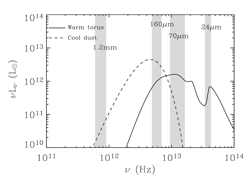
Figure 1.— Illustration of the physical components that dominate at each observed band. The figure shows the SED of a model torus (solid line, from Nenkova et al., 2008a, b) and a cool dust component (dashed line) modelled as a gray body with temperature $T=$40 K and emissivity index $\beta=1.5$ (see Equation 3.2). The observed bands at 24, 70 and 160 $\mu$m, as well as 1.2 mm, are available for all 21 sources and have been marked in gray. This model source is assumed to be at $z=2$ so the bands have been accordingly shifted to the rest-frame frequencies. The relative luminosities of the two components are arbitrary but representative of the sources in this sample. For completeness, the exact torus parameters used are: single-cloud optical depths $\tau_{\rm V}=60$, gaussian angular distribution of clumps around the equator, $\sigma=60$, the number of clouds along a ray in the equatorial plane $N=10$, the ratio of inner to outer torus radius $Y=30$, and the power of the radial density distribution, $q=0$.

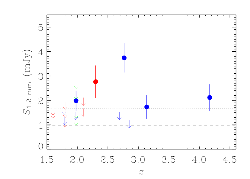
Figure 2.— Flux density, $S_{1.2~{}\rm mm}$, versus redshift $z$ for the sample of obscured quasars. Sources marked in blue have redshifts from optical spectroscopy, those marked in red have redshifts only from their mid-infrared spectra. All limits are 3$\sigma$. The four green sources have no spectroscopic redshifts and have been placed at $z=1.98$, the median value for sources with a spectroscopic redshift. At $z=2$ there are 4 green sources (one detection and three upper limits) and 2 blue sources (one detection and one upper limit). The dotted line represents the approximate flux density limit of the MAMBO observations: $\sim$1.65 mJy. The dashed line shows the value of $\langle S_{1.2~{}\rm mm}\rangle$, the mean flux density for all 21 sources.

Figure 3.— Distribution of observed flux densities. The empty histogram represents the measured flux densities for all sources, the shaded histogram for detections. The distribution is clearly centred on a positive value, and skewed towards the high-flux density end. The solid vertical line shows the stacked mean of all sources, the dashed line the stacked mean for detections, and the dotted line the stacked mean for non-detections.

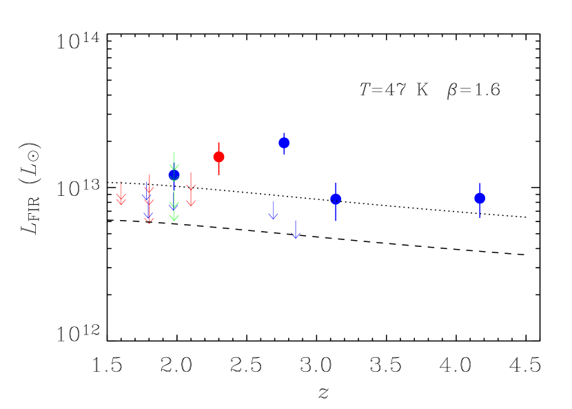
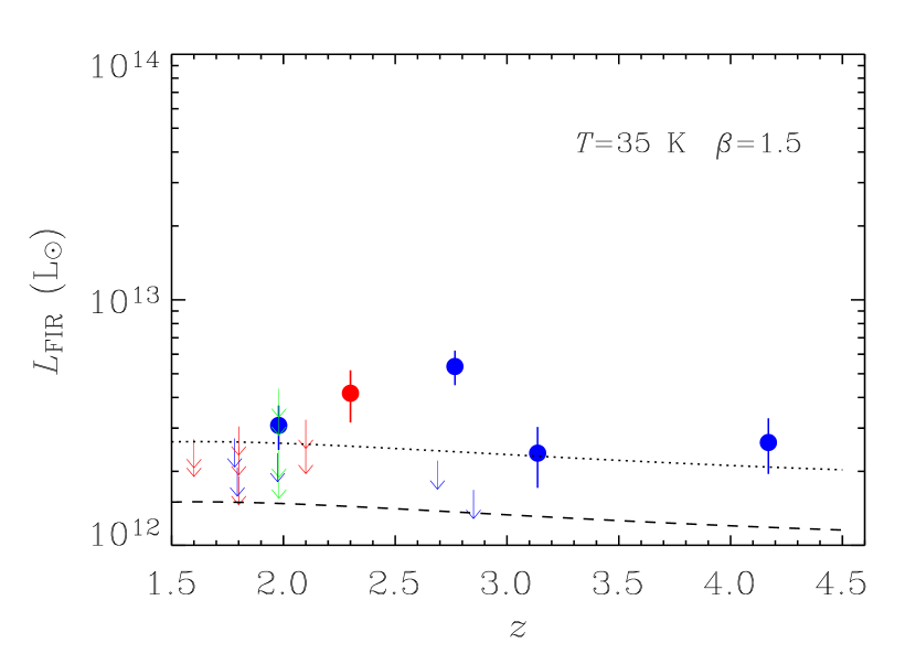
Figure 4.— Far-infrared luminosity, $L_{\rm FIR}$, versus redshift $z$, for the two fiducial gray bodies. Symbols are the same as in Figure 2. The dotted line represents the value of $L_{\rm FIR}$  corresponding to the approximate flux limit, while the horizontal dashed line represents the far-infrared luminosity corresponding to $\langle S_{1.2~{}\rm mm}\rangle$ at each redshift.

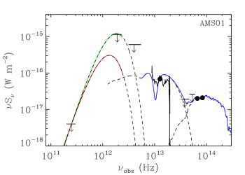
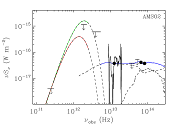
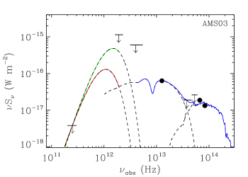
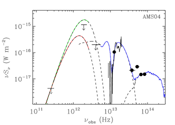
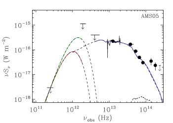
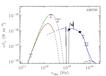
Figure 5.— Spectral energy distributions of the sample of high-redshift obscured quasars. Data points are marked as black points for detections or arrows for limits (left to right): 1.2 mm, 160, 70, 24, 8, 5.8, 4.5, 3.6 $\mu$m  (data from Lacy et al., 2005; Fadda et al., 2006; Frayer et al., 2006, and deeper unpublished IRAC data). All limits are 3$\sigma$. Overlayed in black are also the IRS spectra, when available. The far-infrared SED is modelled by a gray body, as described in Section 3.2. The mid-infrared component is modelled by an unobscured quasar SED with foreground extinction (see Section 4). The dashed lines are the Elvis et al. (1994) quasar SED with a screen of dust (with the value of $A_{\rm V}$  as quoted in Table 3 and using the MW dust model of Pei, 1992) and a $z=0$ elliptical galaxy from Coleman et al. (1980). The quasar SED has been truncated at wavelengths longer than rest-frame 80 $\mu$m. The blue solid line is the sum of both obscured quasar and host galaxy SEDs at wavelengths shorter than 20 $\mu$m, fitted using the data points between 3.6 and 24 $\mu$m  (see Section 4). Source AMS05 has additional data points at 1.2, 1.6 and 2.2 $\mu$m  from Smith et al. (2009).

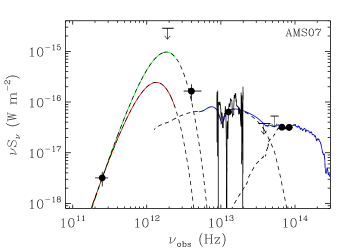
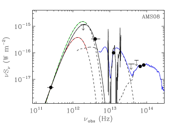
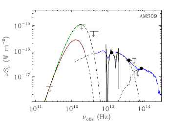
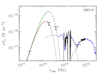
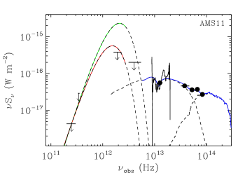
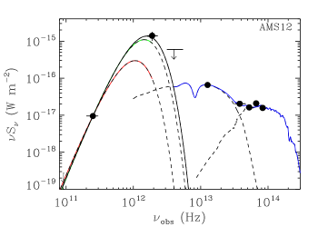
Figure 5.— Continued. Source AMS11 has an extra point at 850 $\mu$m, from the observations of Frayer et al. (2004), while source AMS12 has a limit on the 3 mm flux density from the PdBI observations. Sources AMS08 and AMS12 have an extra gray body overplotted (black solid lines), described by the values in Table 4.

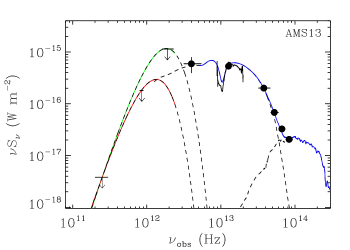
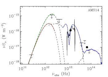
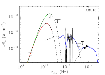
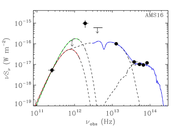
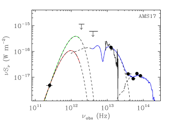
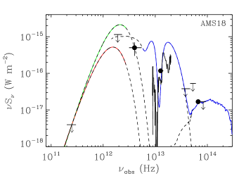
Figure 5.— Continued. Sources AMS13 and AMS16 have additional data at 350 $\mu$m  from the SHARC observations. In addition, AMS16 has a limit on the 3 mm flux density from the PdBI observations.

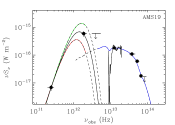
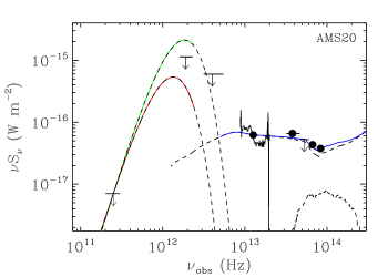
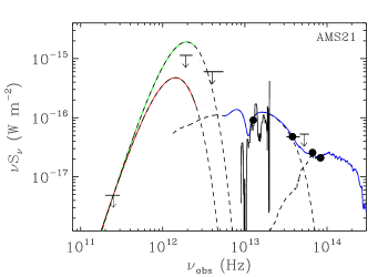
Figure 5.— Continued. Source AMS19 has an extra gray body overplotted (black solid line), described by the values in Table 4.

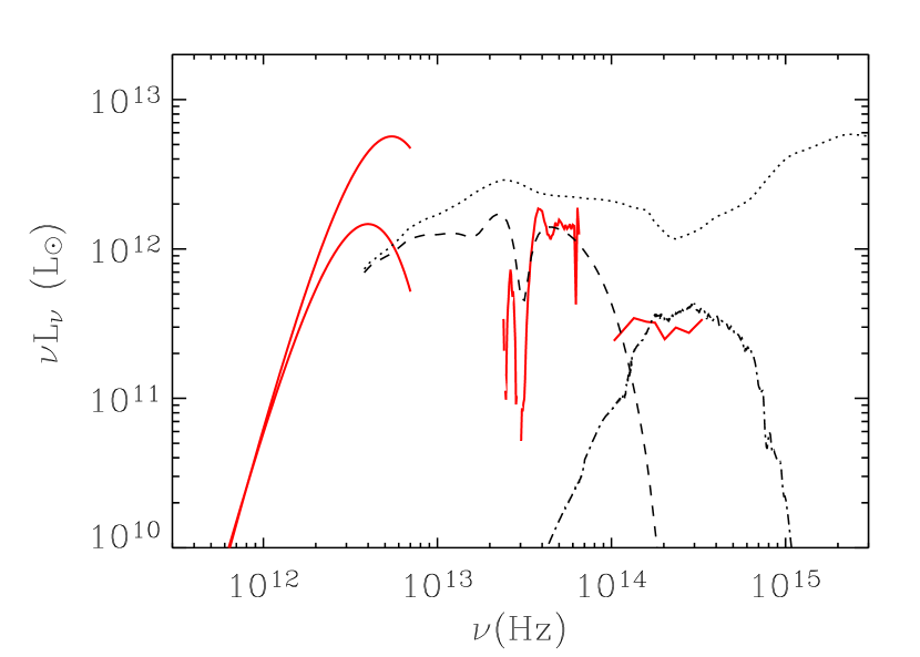
Figure 6.— Mean dust SED for the sources in our sample with spectroscopic redshifts (solid red lines, see Section 5). The near-infrared component is the mean of the observed IRAC photometry ($\nu=1-4\times 10^{14}$ Hz, observed at 3.6-8.0 $\mu$m), the mid-infrared component ($\nu=2-6\times 10^{13}$ Hz) is constructed using the IRS spectra, while the far-infrared component ($\nu\leq 1\times 10^{13}$ Hz) described by either one of the two fiducial gray bodies (the top solid red line has $T=$47 K, $\beta=$1.6, the bottom one has $T=$35 K, $\beta=$1.5). Overplotted for reference are an unobscured quasar SED (dotted line Elvis et al., 1994) as well as the same quasar SED with a screen of MW dust (from Pei, 1992) with the mean $A_{\rm V}$$=32$ (plotted as a dashed line), and a $z=0$ elliptical galaxy Coleman et al. (dash-dotted line, from 1980). This last SED has been normalised to be the progenitor of a present day $\sim 2$$L^{\star}$ galaxy.

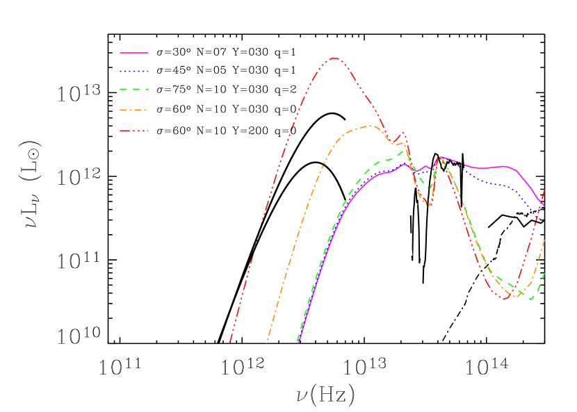
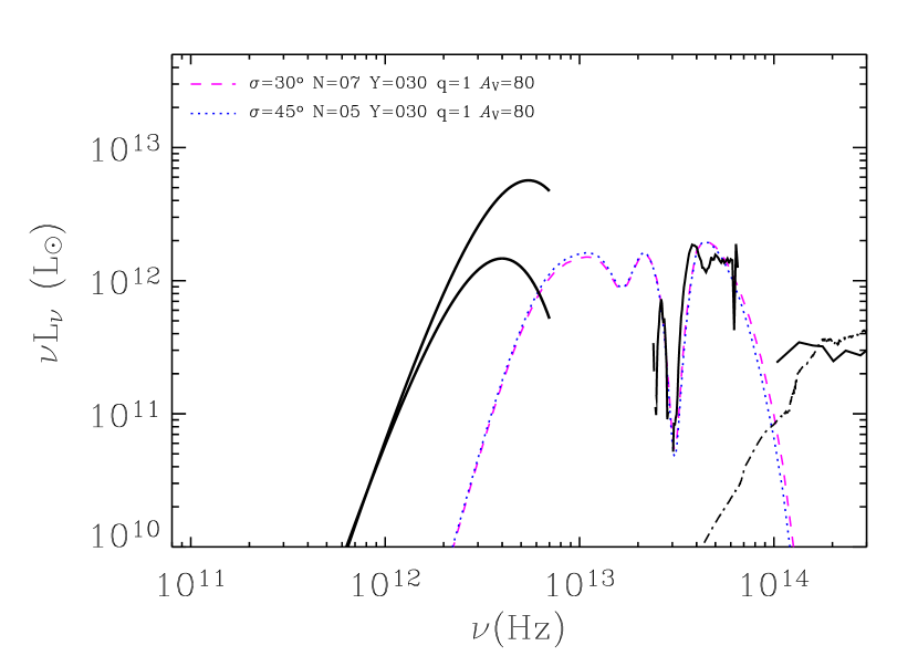
Figure 7.— Comparison of the mean SED (solid black lines) with different clumpy models of AGN tori. The progenitor of a 2$L^{\star}$ galaxy has been overplotted again (dot-dashed line). The clumpy models, from Nenkova et al. (2008a, b), all have single-cloud optical depths $\tau_{\rm V}=60$. Left panel: Different lines show models with varying parameters for the width of the gaussian angular distribution of clumps around the equator, $\sigma$, the number of clouds along a ray in the equatorial plane $N$, the ratio of inner to outer torus radius $Y$, and the power of the radial density distribution, $q$. The models cannot simultaneously reproduce the relatively flat continuum between $1\times 10^{13}$ and $7\times 10^{13}$ Hz, the sudden drop at higher frequencies, the depth of the silicate feature and the millimetre detection. Right panel: Additional extinction from dust along the line of sight has been added to the two flatter clumpy models from the left panel. The emission from this cool dust is represented by the two fiducial gray bodies used throughout this work. The typical quasar SED of our sample can be reasonably reproduced using the clumpy torus models, with foreground extinction $A_{\rm V}$$=80$ and re-emission from a mass of $3\times 10^{8}$ M_⊙  of cool dust. The emission from this cool-dust mass and the foreground extinction are consistent provided the dust is within a 2 kpc radius (using Equation 8 from Section 3.6).

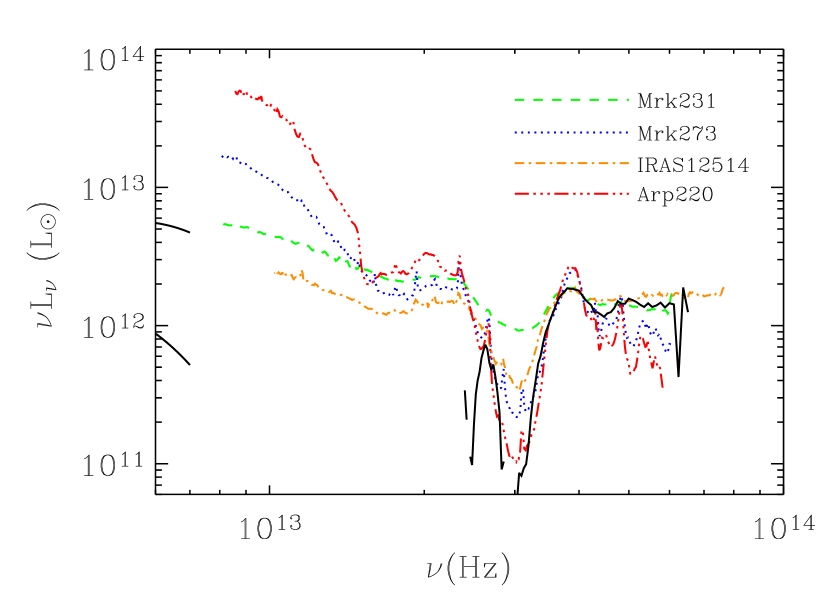
Figure 8.— Comparison of the mid-infrared component of the mean SED (black solid line) with four local ULIRGs: IRAS 12514$+$1027 (hereafter IRAS 12514), Mrk 231, Mrk 273 and Arp 220.

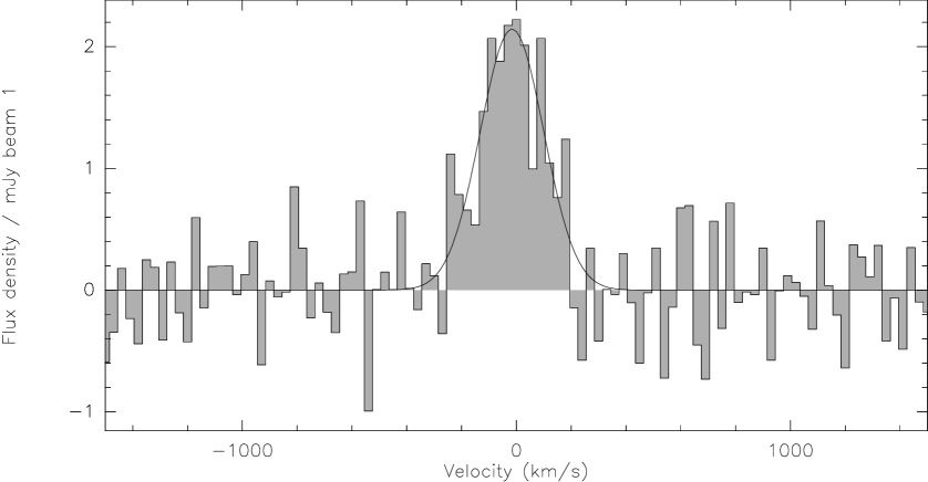
Figure 9.— Spectrum of AMS12 obtained with the Plateau de Bure Interferometer. The line is well fit by a single gaussian centred on -16 km s^-1  ($z_{\rm CO}=2.7668$) with a FWHM of 275 km s^-1. From this gaussian fit, the CO(3-2) line has an integrated flux of 630 mJy km s^-1 corresponding to a frequency-integrated line luminosity of $L_{\rm CO(3-2)}=$3.2$\times 10^{7}$ L_⊙, or a brightness-temperature luminosity of $L^{\prime}_{\rm CO(3-2)}=2.4\times 10^{10}$ K km s^-1 pc².

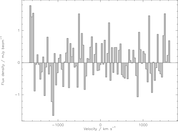
Figure 10.— Spectrum of AMS16 obtained with the Plateau de Bure Interferometer. The frequency was centred on 89.2002 GHz, the expected location of the CO(4-3) rotational transition. The rms noise per 10 MHz bin (33 km s^-1) is 0.65 mJy beam^-1, assuming a box-car CO line shape with full width to zero intensity of 400 km s^-1  and the line to be within the frequency covered, the 3$\sigma$ limit is $\Delta\nu S_{\rm CO}<$230 mJy beam^-1 km s^-1, or $L^{\prime}_{\rm CO(4-3)}<1\times 10^{10}$ K km s^-1 pc² at the redshift of the source.

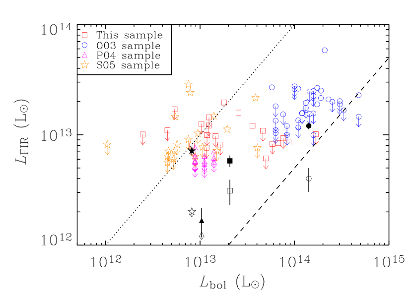
Figure 11.— $L_{\rm FIR}$  vs $L_{\rm bol}$  for the four samples of $z\sim 2$ quasars considered. O03 is the sample presented by Omont et al. (2003), P04 by Page et al. (2004) and S05 by Stevens et al. (2005). Black filled symbols represent the weighted mean of all sources in each sample, black empty symbols represent the weighted mean of non-detections in each sample. The dashed line represents $L_{\rm FIR}$$=0.05$$L_{\rm bol}$, the value found in low-redshift quasars considered by Elvis et al. (1994). For reference, the line $L_{\rm FIR}$$=$$L_{\rm bol}$  has been plotted as a dotted line. For all samples, a gray body with $T=47$ K and $\beta=1.6$ has been assumed to calculate $L_{\rm FIR}$.

References

- Alton et al. (2004) Alton, P. B., Xilouris, E. M., Misiriotis, A., Dasyra, K. M., & Dumke, M. 2004, A&A, 425, 109
- Aravena et al. (2008) Aravena, M., et al. 2008, A&A, 491, 173
- Armus et al. (2007) Armus, L., et al. 2007, ApJ, 656, 148
- Barger et al. (2005) Barger, A. J., Cowie, L. L., Mushotzky, R. F., Yang, Y., Wang, W.-H., Steffen, A. T., & Capak, P. 2005, AJ, 129, 578
- Barger et al. (1998) Barger, A. J., Cowie, L. L., Sanders, D. B., Fulton, E., Taniguchi, Y., Sato, Y., Kawara, K., & Okuda, H. 1998, Nature, 394, 248
- Barvainis (1987) Barvainis, R. 1987, ApJ, 320, 537
- Beelen et al. (2006) Beelen, A., Cox, P., Benford, D. J., Dowell, C. D., Kovács, A., Bertoldi, F., Omont, A., & Carilli, C. L. 2006, ApJ, 642, 694
- Beelen et al. (2004) Beelen, A., et al. 2004, A&A, 423, 441
- Brand et al. (2007) Brand, K., et al. 2007, ApJ, 663, 204
- Chapman et al. (2004) Chapman, S. C., Smail, I., Windhorst, R., Muxlow, T., & Ivison, R. J. 2004, ApJ, 611, 732
- Clavel et al. (2000) Clavel, J., et al. 2000, A&A, 357, 839
- Cole et al. (2001) Cole, S. et al. 2001, MNRAS, 326, 255
- Coleman et al. (1980) Coleman, G. D., Wu, C.-C., & Weedman, D. W. 1980, ApJS, 43, 393
- Croom et al. (2004) Croom, S. M., Smith, R. J., Boyle, B. J., Shanks, T., Miller, L., Outram, P. J., & Loaring, N. S. 2004, MNRAS, 349, 1397
- Dowell et al. (2003) Dowell, C.D., et al. 2003, SPIE, 4855, 73.
- Downes & Solomon (1998) Downes, D. & Solomon, P. M. 1998, ApJ, 507, 615
- Dunne et al. (2003) Dunne, L., Eales, S. A., & Edmunds, M. G. 2003, MNRAS, 341, 589
- Egami et al. (2004) Egami, E., et al. 2004, ApJS, 154, 130
- Elvis et al. (1994) Elvis, M., et al. 1994, ApJS, 95, 1
- Fabian (1999) Fabian, A. C. 1999, MNRAS, 308, L39
- Fadda et al. (2006) Fadda, D., et al. 2006, AJ, 131, 2859
- Frayer et al. (2004) Frayer, D. T., et al. 2004, ApJS, 154, 137
- Frayer et al. (2006) Frayer, D. T., et al. 2006, AJ, 131, 250
- Greve et al. (2005) Greve, T. R., et al. 2005, MNRAS, 359, 1165
- Haas et al. (2004) Haas, M., et al. 2004, A&A, 424, 531
- Houck et al. (2005) Houck, J. R., et al. 2005, ApJ, 622, L105
- Hughes et al. (1998) Hughes, D. H., et al. 1998, Nature, 394, 241
- Isobe & Feigelson (1990) Isobe, T. & Feigelson, E. D. 1990, in Bulletin of the American Astronomical Society, Vol. 22, 917
- Kennicutt (1998) Kennicutt, Jr., R. C. 1998, ARA&A, 36, 189
- Klamer et al. (2005) Klamer, I. J., Ekers, R. D., Sadler, E. M., Weiss, A., Hunstead, R. W., & De Breuck, C. 2005, ApJ, 621, L1
- Klöckner et al. (2009) Klöckner, H. ., Martinez-Sansigre, A., Rawlings, S., & Garrett, M. A. 2009, in press., (ArXiv:0905.1605)
- Kovács (2006) Kovács, A. 2006, PhD thesis, Caltech.
- Kovács et al. (2006) Kovács, A., Chapman, S. C., Dowell, C. D., Blain, A. W., Ivison, R. J., Smail, I., & Phillips, T. G. 2006, ApJ, 650, 592
- Kreysa et al. (1998) Kreysa, E., et al. 1998, SPIE, 3357, 319
- Lacy et al. (2007) Lacy, M., Sajina, A., Petric, A. O., Seymour, N., Canalizo, G., Ridgway, S. E., Armus, L., & Storrie-Lombardi, L. J. 2007, ApJ, 669, L61
- Lacy et al. (2005) Lacy, M. et al. 2005, ApJS, 161, 41
- Lawrence & Elvis (1982) Lawrence, A. & Elvis, M. 1982, ApJ, 256, 410
- Leong (2005) Leong, M.M. 2005, URSI Conf. Sec., J3-J10,426
- Levenson et al. (2007) Levenson, N. A., Sirocky, M. M., Hao, L., Spoon, H. W. W., Marshall, J. A., Elitzur, M., & Houck, J. R. 2007, ApJ, 654, L45
- Lutz et al. (2005) Lutz, D., Yan, L., Armus, L., Helou, G., Tacconi, L. J., Genzel, R., & Baker, A. J. 2005, ApJ, 632, L13