AKARI and BLAST Observations of the Cassiopeia A Supernova Remnant and Surrounding Interstellar Medium

Abstract

We use new large area far infrared maps ranging from 65-500 $\mu$m obtained with the AKARI and the Balloon-borne Large Aperture Submillimeter Telescope (BLAST) missions to characterize the dust emission toward the Cassiopeia A supernova remnant (SNR). Using the AKARI high resolution data we find a new “tepid” dust grain population at a temperature of $\sim 35$ K and with an estimated mass of 0.06 M_⊙. This component is confined to the central area of the SNR and may represent newly-formed dust in the unshocked supernova ejecta. While the mass of tepid dust that we measure is insufficient by itself to account for the dust observed at high redshift, it does constitute an additional dust population to contribute to those previously reported. We fit our maps at 65, 90, 140, 250, 350, and 500 $\mu$m to obtain maps of the column density and temperature of “cold” dust (near 16 K) distributed throughout the region. The large column density of cold dust associated with clouds seen in molecular emission extends continuously from the surrounding interstellar medium to project on the SNR, where the foreground component of the clouds is also detectable through optical, X-ray, and molecular extinction. At the resolution available here, there is no morphological signature to isolate any cold dust associated only with the SNR from this confusing interstellar emission. Our fit also recovers the previously detected “hot” dust in the remnant, with characteristic temperature 100 K.

Keywords: Star Formation — Cosmology: dust formation — supernovae: individual (Cas A)

1. Introduction

Determining the origin of cosmic dust is fundamental to our understanding of many astronomical processes, including star formation and galaxy evolution. Galaxies and quasars at high redshift have been found to contain large amounts of dust ($\geq 10^{8}$ M_⊙; Dunlop et al., 1994; Archibald et al., 2001; Isaak et al., 2002; Priddey et al., 2008), at a time when the Universe was only about one tenth of its present age. The main source of dust injection within our Galaxy is thought to be the stellar winds of stars on the asymptotic giant branch (AGB) of the Hertzsprung-Russell (HR) diagram (Morgan and Edmunds, 2003). Stars at this early epoch would not have been able to reach the AGB phase in the available time, and therefore cannot be the source of the observed dust. Heavy elements are produced in the explosions of supernovae (SNe) and, for several years, models have predicted that considerable amounts of fresh dust (0.1-1 M_⊙) could also be produced (Kozasa et al., 1991; Woosley and Weaver, 1995; Clayton et al., 1999; Todini and Ferrara, 2001). The life cycle of high mass stars ($>$8 M_⊙), the progenitors of type II SNe, is sufficiently short for SNe to occur within the required timescales. As a result, SNe have been proposed as a possible solution for the origin of the dust seen at high-redshift. However, in order for SNe to generate sufficient dust mass to fill this gap, each supernova would need to generate 0.4-1 M_⊙ dust (Dwek et al., 2007). This quantification does not account for dust grain destruction within the supernova, thereby making it a lower bound.

In seeking evidence regarding this hypothesis, the focus has been on dust detectable in SNe and supernova remnants (SNR), as reviewed briefly below. However, it seems less well appreciated that injection is only part of the story. Draine (2003) reviews the often-ignored arguments that, at least in our Galaxy, the interstellar dust is continually processed on a timescale $3\times 10^{8}$ yr and most of its mass is formed in the interstellar medium. Nevertheless, injected dust is critical at least as seeds for further evolution of the dust population.

Studies of SNe find only trace amounts of dust in the hot ejecta, with typical masses of order 10^-4 M_⊙ (Dwek et al., 1987; Lagage et al., 1996; Arendt et al., 1999; Ercolano et al., 2007; Meikle et al., 2007). Dust studies in SNR appear more promising, a prime example being Cassiopeia A (Cas A). Cas A is the remnant of a type IIb supernova event which occurred around AD 1680 (Raymond, 1984; Thorstensen et al., 2001; Fesen et al., 2006a; Krause et al., 2008). The progenitor star is believed to have had a mass greater than 20 M_⊙ (Pérez-Rendón et al., 2002), and the remnant is at a distance $D\sim 3.4$ kpc (Reed et al., 1995). Early observations of Cas A made with IRAS (Neugebauer et al., 1984) and ISO (Kessler et al., 1996) did not extend to longer wavelengths, and therefore detected only the “hot” ($\sim$100 K) dust component, whose mass seemed insufficient to provide the levels of dust seen in high redshift galaxies. The low angular resolution also made the study of sub-structure in the remnant at intermediate wavelengths difficult. The Spitzer Space Telescope (Werner, 2006) has been used to study Cas A (Hines et al., 2004; Krause et al., 2004; Ennis et al., 2006). Most recently Rho et al. (2008), exploiting the angular and spectral resolution achieved with the Spitzer infrared spectrograph (IRS; Houck et al., 2004), find between 0.020 – 0.054 M_⊙ of hot dust. This is an order of magnitude greater than that previously measured and they conclude that, within modeling uncertainties for galaxy evolution, this could be sufficient to explain at least the lower limit to the dust levels in high-redshift galaxies presented by Isaak et al. (2002).

Much more controversial is the question of a “cold” dust component in the SNR, because of the issue of contamination by line-of-sight interstellar emission from dust which is also cold ($\sim$16 K; § 5). Dunne et al. (2003), using data from the Submillimetre Common User Bolometer Array (SCUBA; Holland et al., 1999), find evidence for $2-4\,{\rm M\mbox{${}_{\odot}$}}$ of dust in Cas A at a temperature of $\sim$18 K, significantly more than the mass of hot dust. Using the same methodology, Morgan et al. (2003) find $\sim$1 M_⊙ of cold dust in Kepler’s supernova remnant, a thousand times greater than previous measurements for this SNR. Both of these remnants are sufficiently young for the dust observed to be freshly formed in the remnant, rather than being material swept up from the ISM by the shock-wave (Dickel et al., 1988; Hughes, 1999; Wright et al., 1999). More recently, Dunne et al. (2009) presented further evidence for cold dust in Cas A using SCUBA polarization data. These show dust emission polarized in an orientation consistent with that of the magnetic field deduced from the radio synchrotron emission, suggesting the detected dust is in the SNR. They find a conservative lower limit for this dust mass of 1 M_⊙. They also attribute apparent depolarization at the brightest feature to dilution by line of sight interstellar emission.

Dwek (2004) has argued that the mass estimates in Dunne et al. (2003) exceed the total anticipated mass ejection of Cas A and suggest that if the submillimeter observations are valid they might instead imply the presence of a much smaller amount of dust which is a much more efficient millimeter wavelength radiator, such as iron needles. The alignment of such needles could affect the polarization.

By correlating cold dust emission with molecular line absorption against the SNR synchrotron emission, Krause et al. (2004) argued that the dust is, in fact, associated with a molecular cloud located along the line of sight to the SNR. Molecular emission has also been studied in this direction (e.g., Liszt and Lucas 1999), showing that the cloud(s) extend well beyond the SNR itself. Krause et al. estimate the fresh dust yield within Cas A to be at least an order of magnitude lower than that found by Dunne et al. (2003). Even so, this would still provide the predominant dust mass in Cas A, bolstering the possibility of explaining the quantities of dust seen at high-redshift.

The emission from cold dust peaks in the far-infrared and submillimeter and so neither SCUBA, on the long wavelength side, nor Spitzer, on the short side, is ideal for isolating a cold dust component. Near the thermal peak, the best large scale maps covering Cas A and its environs are from the Multiband Imaging Photometer for Spitzer (MIPS; Rieke et al., 2004) at 160 $\mu$m (Krause et al., 2004) and from the ISO Serendipity Survey at 170 $\mu$m (Stickel et al., 2007). Neither map has full coverage, with MIPS missing data on small scales and ISOSS on larger.

We observed Cas A using the Far-Infrared Surveyor (FIS; Kawada et al., 2007) instrument on-board AKARI. We obtained fully-sampled images of sub-arcminute resolution covering a wide area surrounding Cas A in four photometric bands from 50 to 180 $\mu$m. This is the wavelength range over which the emission from newly formed hot dust becomes faint and emission from cold dust begins to dominate. Therefore, these AKARI FIS images are very useful for investigating the presence of colder components of dust in the remnant.

The Balloon-borne Large-Aperture Submillimeter Telescope (BLAST; Pascale et al., 2008) was also used to observe the Cas A region at 250, 350, and 500 $\mu$m. These bands fill in the cold dust spectral energy distribution (SED) on the long wavelength side of the peak. The high mapping speed of BLAST means it was possible to cover a large area surrounding the SNR, giving data for both the SNR and the interstellar cloud structure in the surrounding region.

By contrast, the prior SCUBA maps are of a small area and involve deconvolution of a three-beam chopping pattern which reconstructs large scale power poorly. AKARI and BLAST have the advantage that, like Spitzer, they are not required to perform chopped observations. As a result, our new maps are sensitive to the large scale structure present in the Cas A field. The relatively large area of these maps, coupled with their sensitivity and wavelength coverage, make them ideal for investigation of cold dust emission from Cas A and the interstellar clouds.

We describe the AKARI and BLAST observations in § 2. Several distinct sources of emission are distinguishable in these maps. Taking advantage of the AKARI spatial resolution, in § 3 we identify a new morphologically compact source of “tepid” ($\sim$35 K) dust emission centered on the SNR whose spectrum is also distinct, peaking between the SED peak of the hot dust in the SNR and that of the cold dust. In § 4 we perform aperture photometry on the maps in the region of the Cas A SNR. The resulting global SED further illustrates the different spectral components and shows that without the additional morphological information it is not possible to unambiguously distinguish the tepid dust component. In § 5 we fit the six-band AKARI-BLAST data with a simple spectral model to make column density and temperature maps for the cold dust. These clearly illustrate the confused nature of cold dust emission on the line of sight to the SNR. In § 5.1 the derived column density on the line of sight is compared to that obtained by other techniques. We present our conclusions in § 6.

2. Data

2.1. AKARI

The AKARI FIS observations of Cas A were obtained on 2007 July 19 (Obs ID: 1402802). FIS has four photometric bands at 65, 90, 140, and 160 $\mu$m; two wide bands, 90 and 140 $\mu$m, and two narrow bands, 65 and 160 $\mu$m (Kawada et al., 2007). FIS carried out a ‘slow-scan’ observation of Cas A with a scan speed of 15^′′ s^-1 and a reset interval of 1 s. The size of the detector pixels was $26\farcs 8$ for the 65 and 90 $\mu$m bands and $44\farcs 2$ for the 140 and 160 $\mu$m bands, approximately equal to the beam size. The area covered for Cas A is 40^′ $\times$ 12^′. During the observation, the dark signal was measured five times, at the beginning, at the turning points of each scan leg, and at the end of the observation, by closing a cold shutter. The variation of responsivity was monitored by using an internal calibrator.

The raw data were processed with the official FIS slow-scan toolkit (Verdugo et al., 2007). The removal of bad data as well as cosmic-ray hits and the correction of integration ramps were made in the pipeline. During the responsivity variation correction, dark current subtraction and flat fielding were performed. Since the dark level for 160 $\mu$m was overestimated due to a large change of responsivity, the 160 $\mu$m data were excluded in this paper. The sigma-clipping method was applied to calibrated signals within the size of a detector pixel in order to remove small undetected glitches as well as other artifacts. The image was reconstructed with the assumption that a pixel value represents the uniform intensity over the pixel surface in the fine image grid. The average value was taken from the multiple values in the image grid. The absolute calibration was accomplished by comparison with data from the Diffuse Infrared Background Experiment (DIRBE; Silverberg et al., 1993). For point-source calibration, the uncertainties of flux calibration are no more than 20% for the two short wavelength bands, and 30% for the 140 $\mu$m band (Kawada et al., 2007).

2.2. BLAST

BLAST made a ‘cap’ observation (Pascale et al., 2008) of Cas A during its first long duration balloon flight from Kiruna, northern Sweden, in June 2005. Maps were made with a slew rate of 6’ s^-1 in azimuth, and a slow drift in elevation which produced a scan line spacing of $3\farcm 25$ (about half an array width). Due to flight time limitations, it was only possible to perform 1.25 complete scan maps. The final images are $\sim$40^′ $\times$ 60^′ in size. The maps were made with the SANEPIC algorithm (Patanchon et al., 2008) and were calibrated using the procedure discussed in Truch et al. (2008).

Although the mirror diameter was 2 m, the BLAST05 SANEPIC maps had only 3^′ full-width at half-power resolution due to an anomalous telescope beam, corrupted by some uncharacterized combination of mirror distortion and de-focus (Truch et al., 2008) (this was corrected for the BLAST06 flight). Nevertheless, these maps have high signal-to-noise and are oversampled with 20^′′ pixels, so that Lucy-Richardson (L-R) deconvolution can be used to improve the resolution significantly (Roy et al. 2009, in preparation). After 32 iterations, the L-R maps used here have point spread functions of $1\farcm 3$, $1\farcm 6$, and $1\farcm 9$ in the 250, 350, and 500 $\mu$m bands, respectively, determined by measuring the size of a point source in the maps. While greatly improved, these are still not as small as the nominal BLAST values of $0\farcm 5$, $0\farcm 66$, and 1^′, or the even smaller values anticipated with the Herschel Space Observatory.

The AKARI maps have a well-established zero point, but the BLAST SANEPIC processing filters the lowest spatial frequencies and produces maps with zero mean value. In order to model the column densities and temperatures in § 5, we need to establish the true zero points of each BLAST map. As described below, we use DIRBE maps of the region to establish the appropriate mean value of the 250 $\mu$m BLAST map, and we use correlations between the BLAST maps to establish the zero points at the two longer BLAST wavelengths. In practice these two steps are done simultaneously.

Although the DIRBE beams are $1.3\times 10^{-4}$ sr, much too large to resolve the structure around Cas A (there is of order one beam in the entire BLAST map), the experiment was explicitly designed to measure total flux and is therefore ideal for establishing the absolute intensity in each map. For the Cas A position the DIRBE intensities are 24.5, 86.8, 191.2 and 142.9 MJy sr^-1 at wavelengths of 60, 100, 140 and 240 $\mu$m. These values are plotted in Figure 1.

Figure 1.— Mean values of the maps within a DIRBE beam. The DIRBE photometry used to set the zero-points in the BLAST maps is shown as triangular data points, and the relative amplitudes of the BLAST mean values, as described in the text, are shown as diamonds. The solid curve is the sum of a cold dust curve with emissivity index $\beta=2$ and adjustable temperature. Also shown is a curve for non-equilibrium dust emission from small grains with $\beta=2$, $T=40$ K and an amplitude 14% of that of the cold dust. The amplitude and temperature of the cold dust is chosen to minimize the deviation of this sum from the data points at the locations of the vertical error bars. The size of those error bars shows the assumed constant relative uncertainty corresponding to $\chi^{2}_{\nu}=1$ for the best fit. The pluses show mean values from the AKARI maps well away from the Cas A SNR, and the agreement is excellent. The inferred mean zero-point values appropriate to the three BLAST bands are written next to each point.

The morphology of the structure in the BLAST maps, shown in Figure 2, are generally similar to each other, indicating that the SED of the interstellar dust is comparatively uniform across the region. The Pearson correlation coefficients of the 350 and 500 $\mu$m maps to the 250 $\mu$m map are $r=0.98$ and $0.97$, respectively. The measured slopes, $A$, for the relation $\hat{I}_{\lambda}=A\hat{I}_{250}$ are 0.51 and 0.28, respectively, for $\lambda=350$ and $500~{}\mu$m, where BLAST map intensities, $\hat{I}_{\lambda}$ have zero mean and have been measured on maps with the region of the Cas A SNR masked out. In the simple picture that the intensity variation within the maps is dominated by variations in column density from place to place, these linear relations should extrapolate to the origin if the maps had correct zero points, and so knowledge of the absolute intensity in any one BLAST band would allow inference of the zero points of the other two maps.

As described in § 5, however, there is a mild anti-correlation of temperature and column density: the dust in the dense arms of the molecular cloud is approximately 2 K cooler than the dust in the less dense gas surrounding them. This biases the measured slopes upward by 7% and 11% at 350 and 500 $\mu$m.

The BLAST slopes, after correction for this small bias, are also plotted in Figure 1, relative to the 250 $\mu$m point on the solid curve. This curve was obtained by fitting to the DIRBE fluxes at 100, 140, and 240 $\mu$m and the relative BLAST amplitudes at 350 and 500 $\mu$m, minimizing $\chi^{2}$ while varying the amplitude of the curve and the temperature of the cold dust. We assume the same fractional uncertainty in each band. The solid error bars in the figure denote the bands used in the fit, and the size of the error bars has been adjusted post-fit to show the fractional uncertainty which would produce a reduced $\chi^{2}_{\nu}=1$. The cold dust temperature was found to be 16.7 K. In order to accommodate the 60 $\mu$m data, the curve includes a contribution of non-equilibrium emission (Desert et al., 1990; Li and Draine, 2001) from very small dust grains (VSGs) at an assumed temperature of 40 K whose peak amplitude has been set to be 14% of that of the cold dust component. However, the 60 $\mu$m data are not used in the fitting procedure. Both the cold dust and the non-equilibrium components are assumed to have power law emissivities, $\epsilon\propto\nu^{\beta}$ with $\beta=2$. Changing $\beta$ to 1.5 does not improve the quality of fit, nor does it alter the BLAST zero points by more than a few percent.

As a check, after the above fitting procedure was complete, the results were compared to mean values from the AKARI maps, which are shown as pluses in Figure 1. The agreement is excellent. The BLAST maps presented in Figure 2 have had the correct zero points applied.

2.3. Maps

Figure 2 presents the AKARI 65, 90, and 140 $\mu$m and BLAST 250, 350, and 500 $\mu$m maps. All maps are centered on the same location, are smoothed to a common resolution of $1\farcm 9$, and are displayed with the identical range of brightness.

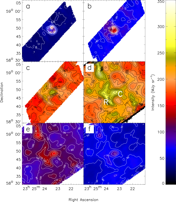
Figure 2.— AKARI 65, 90, and 140 $\mu$m (a–c) and BLAST 250, 350, and 500 $\mu$m (d–f) maps of the Cas A SNR and surrounding ISM, brought to a common resolution of $1\farcm 9$ and centered on the SNR. All maps are displayed with the same intensity scale. Contours are at the native resolution, in steps of 10 MJy sr^-1. The letters C and R label the line of sight elliptical “cloud” and “ridge” features described in the text above.

The relative intensity of emission from the SNR and interstellar clouds varies significantly across the six bands. In the 65 $\mu$m image (Figure 2a) the SNR clearly dominates the map, with the cloud structure barely visible. Hot dust emission arises in the shell of the SNR where there is a reverse shock. This is evident in the shortest wavelength maps in the bright sources along a ring at the apparent SNR outer edge. To illustrate the spectral signature, the brightness at the location corresponding to the brightest peak in the 65 $\mu$m map minus the local background outside the SNR is plotted in Figure 3. A point at 24 $\mu$m is included to suggest the many short-wavelength data that are available (§ 4). When modeled as a simple single-temperature modified blackbody, the hot dust temperature $T_{\rm{H}}$ is $\sim 90$ K ($\beta=2$). Note that this is a great simplification. Adopting a lower $\beta$ would broaden the spectrum, possibly accounting for an underlying intrinsic temperature distribution. Nevertheless, $T_{\rm{H}}$ is in the range found by the more detailed models by Rho et al. (2008).

Figure 3.— Illustrative SEDs of four distinguishable sources of emission (not co-spatial). The “hot” dust spectrum, shown as triangles, is the intensity in each map taken at the location of the peak of the 65 $\mu$m map, $\alpha=23^{h}23^{m}.4$, $\delta=58^{\circ}50^{\prime}.1$ (J2000) minus the local background measured at $23^{h}23^{m}$, $+58^{\circ}45^{\prime}$. The illustrative curve near these points is a $\beta=2$ modified blackbody at $T=92$ K. “Cold” dust (diamonds) is represented by the intensity of the “ridge” in the interstellar cloud structure to the south-east at $23^{h}50^{m}$, $+58^{\circ}44^{\prime}$, minus the respective map average. A $T=15$ K, $\beta=2$ modified black body is drawn to guide the eye. The pluses show the intensity of a “tepid” dust Gaussian central contribution, determined in § 3. The two curves shown ($\beta=1$, $T=41$ K, dashed; and $\beta=2$, $T=33$ K, dot-dashed) fit the data equally well. The lower solid curve shows the synchrotron spectrum measured at $23^{h}23\fm 2$, $+58^{\circ}48\farcm 8$, the brightest peak in the west of the SNR in the 86 GHz map by Liszt and Lucas (1999), and extrapolated using spectral index $-0.72$.

The SNR is also dominant in the AKARI 90 $\mu$m image (Figure 2b). However, the emission ceases to be confined to a simple ring. The brightness at the center of the SNR rises slightly going from 65 $\mu$m to 90 $\mu$m, which is not consistent spatially or spectrally with emission from either the hot or the cold dust component described below. In § 3 we present an analysis of the higher resolution AKARI data to estimate the properties of this new source of intermediate temperature “tepid” dust emission (see resulting SED in Figure 3).

The brightness of the interstellar emission increases at the longer wavelengths, demonstrating that the dust there is at a lower temperature than in the SNR. This “cold” dust emission peaks between the 140 and 250 $\mu$m data (Figs. 2c and 2d), and following a cold greybody SED recedes in the two longest wavelength maps (nevertheless, it is still detected with high signal to noise). The morphology of the cloud structure, both peaks and valleys, is clearest in the 140 – 350 $\mu$m maps (Figs. 2c – 2e). Near the peak of the cold dust SED, the SNR does not stand out as a special feature in the map. There is a brighter cold cloud to the north-east in the extended BLAST maps. Closer to the SNR, there is a bright “ridge” of interstellar emission to the south-east and another elliptical “cloud” beginning to the west outside the remnant and appearing to project across its face. These two features are labelled “R” and “C” in Figure 2d respectively. It is clear that any emission associated with a possible component of fresh cold dust within the SNR will be highly confused by line of sight interstellar emission; this particular interstellar cloud will be called the “line of sight cloud”. The temperature of the cold dust throughout the map is $\sim 16$ K (§ 5). A representative SED is shown in Figure 3 for the molecular cloud ridge to the south-east of the SNR.

The diffuse interstellar emission across the 65 – 90 $\mu$m maps is generally too strong to be modeled along with the long wavelength emission as a single-temperature modified blackbody. It is attributed to the above-mentioned non-equilibrium emission by VSGs (§ 2.2).

Synchrotron emission from relativistic electrons accelerated in the SNR has been mapped extensively, including in the millimeter (Liszt and Lucas, 1999; Wright et al., 1999). The synchrotron power-law SED rises smoothly toward longer wavelengths, and so eventually dominates over the falling dust spectrum. This is already becoming evident in our 500 $\mu$m BLAST map, where the SNR has recovered in relative brightness compared to the interstellar emission. By 850 $\mu$m (SCUBA), the synchrotron emission is dominant. A representative SED is shown in Figure 3 for the synchrotron peak in the west of the SNR. This is drawn for a power-law spectral index $\alpha=-0.72$, near that found by Rho et al. (2003). Spectral index variations across the face of the SNR (Rho et al., 2003; Dunne et al., 2009) and with frequency (Atoyan et al., 2000) are possible, but not critical for the analysis here.

3. Tepid Dust Interior to the SNR

As discussed above, there is well-documented hot ($\sim 100$ K) dust in a broken ring closely associated with the reverse shock and the X-ray emitting plasma (Rho et al., 2008). However, toward the core in the ejecta that has yet to be overrun by the reverse shock there could be cooler dust that can be detected only at longer wavelengths (Dwek and Werner, 1981; Mezger et al., 1986). Its minimum temperature would be set by the ambient radiation field and so it would be at least as warm as the surrounding interstellar dust.

To track “tepid” or intermediate temperature dust which is neither the hot SNR ring component nor cold interstellar emission, the optimal spectral region is 90 – 160 $\mu$m. Indeed, using multi-wavelength (60, 100, 170, 200 $\mu$m) ISOPHOT images, Tuffs et al. (2005) presented evidence for emission from such tepid dust in the un-shocked ejecta in two ways: (i) the morphology of the 100 $\mu$m map shows more central emission than expected from the hot dust component which dominates at 60 $\mu$m, indicating a cooler centrally-peaked component, and (ii) the 170/200 brightness ratio is peaked on the SNR rather than extending with the band of interstellar emission well beyond the SNR to the west, indicating an emission component associated with the SNR that is warmer than the cold interstellar dust. We have confirmed these qualitative findings using the ISOPHOT pipeline-processed data from the ISO archive.

The AKARI angular resolution and wavelength coverage are ideally suited for pursuing approach (i) to the next level, using a “spectrum-informed clean” technique. Like the 60 $\mu$m ISO image, the 65 $\mu$m AKARI image is dominated by the ring component. This can be isolated by subtracting the local background of about 55 MJy sr^-1. This “background-subtracted” map, a hot dust template, can then be scaled, following a hot dust SED, and subtracted from the background-subtracted 90 $\mu$m image. Choosing the SED so as to remove (i.e., “clean”) the morphological signature of the hot dust ring, the striking result is an extended residual feature at 90 $\mu$m centered at $23^{h}23^{m}29^{s}$, $+58^{\circ}48^{\prime}33^{\prime\prime}$ (J2000). To the accuracy available here, this direction is probably indistinguishable from the direction to the center of the SNR. The shape of the feature is well approximated by a Gaussian of FWHM 2^′ which is substantially larger than the beam (37^′′) though smaller than the SNR. The central surface brightness of this residual is about 20 MJy sr^-1, which can be compared to the total of 133 MJy sr^-1 in this same direction. Following the same procedure with the 60 and 100 $\mu$m pair of ISO images produces a residual of very similar size and position, with central surface brightness 27 MJy sr^-1. This is an important check, because the images are not completely free of striping. This quantifies the emission component identified by Tuffs et al. (2005) by its relative morphology.

An interesting question is whether this extended Gaussian component can be seen in the short wavelength images that have been used to generate the hot dust template. Depending on the three-dimensional geometry, there will be some hot dust emission projected on the central line of sight, though a peaked Gaussian arising in this way would seem unusual. Furthermore, at 60 and 65 $\mu$m the surface brightness toward the center is not only brighter than the background, but compared to the hot dust ring is relatively brighter than is the case at shorter wavelengths such as in the archival MIPS 24 $\mu$m image (convolved to the same resolution). This is also the conclusion of Rho et al. (2008) based on the MIPS 70 $\mu$m image (Hines et al., 2004). Therefore, to probe this more probable alternative, we assume that the central emission in the background-subtracted 65 $\mu$m map can be attributed entirely to this Gaussian, which then would have a peak brightness of 33 MJy sr^-1.

Subtracting this Gaussian component from the background-subtracted 65 $\mu$m map produces a new hot dust template with a larger dip in the middle. Therefore, when this is subtracted from the 90 $\mu$m map, the Gaussian residual is still there, but with a larger amplitude, 42 MJy sr^-1 (see Figure 4). Analysis of the 60 – 100 $\mu$m ISO pair yields a similar result. We consider this to be an upper limit. The 60 – 65 to 90 – 100 $\mu$m color temperature is about 33 K ($\beta=2$) or 41 K ($\beta=1$).

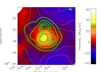
Figure 4.— AKARI 90 $\mu$m background-subtracted map of the Cas A SNR from which the hot dust emission has been removed (“cleaned”). Heavy contours from the AKARI 65 $\mu$m map show the position of the hot dust ring and the thin contours from the BLAST 250 $\mu$m map show the cold dust emission including the “line of sight cloud” and the “ridge” to the south-east.

Proceeding with this “spectrum-informed cleaning”, now removing both the hot dust and tepid Gaussian components from the 90 or 100 $\mu$m images, we find toward the SNR only a fainter residual in the west, (coincidentally) at the projected distance of the reverse shock, and extending to the southeast, a morphology crossing the remnant that is qualitatively consistent with being interstellar. The latter morphological component (called the “line of sight cloud” in § 2.3 and below) can be seen directly in the 250 and 350 $\mu$m BLAST images (Figure 2), even without any component subtraction, and in the cold dust column density map (Figure 6b below in § 5). As in the MIPS 160 $\mu$m image (Krause et al., 2004) and the long wavelength ISO maps, this extends to the west well outside the SNR.

In the two intermediate-wavelength images (AKARI 140 $\mu$m in Figure 2c; ISO 160 $\mu$m) the hot dust ring component is no longer obvious. But in both there are two distinguishable peaks of emission, toward the center and the band from the western peak extending to the southeast. The Gaussian component could be as bright as 35 MJy sr^-1 (with the second alternative hot dust template), fairly consistent with extrapolation of the tepid dust SED from shorter wavelengths. Compared to the situation at 100 $\mu$m, the residual line of sight cloud projected on the SNR and the adjacent “ridge” of interstellar emission to the south-east have become brighter, as expected for cold dust.

The peak amplitude of this central Gaussian feature, from the three maps where it can be distinguished, is plotted as pluses in Figure 3. Two modified blackbody curves plotted there ($\beta=2$, $T=33$ K and $\beta=1$, $T=41$ K) describe the measured amplitudes equally well. Both indicate only a small flux from this component at longer wavelengths where the combination of coarser BLAST angular resolution and comparatively intense line of sight emission have not allowed direct measurement.

As mentioned above, hot dust emission is correlated with X-ray line and continuum emission and infrared line emission from the shocked gas. It is therefore interesting to ask if there is any tracer of the plasma that is coincident with the central tepid dust emission. Smith et al. (2009) show maps of several lines from different ions tracing different physical conditions in the SNR. The [Si II] 34.8 $\mu$m emission in their Figures 2 and 7 is from the unshocked ejecta in the interior of the SNR inside the reverse shock boundary (see their Figure 4). The peak position of this central emission appears to be consistent with the location of our Gaussian component. L. Rudnick (private communication) finds from a map of the central low density areas convolved to the AKARI resolution that the FWHM is comparable too.

Identification of this tepid dust Gaussian component clearly depends on clues from how the SNR morphology changes with wavelength. Using the higher-resolution multi-wavelength morphological information anticipated from Herschel, it will be very interesting to characterize this component in more detail for comparison with such (3-dimensional) tracers.

3.1. Mass of Tepid Dust

Dust emission maps record surface brightness $I_{\nu}$ which in turn depends on the dust mass column density $M_{d}$ through

$$M_{\rm{d}}=I_{\nu}/\kappa_{\nu}B_{\nu}(T_{\rm{d}}),$$ (1)

where $\kappa_{\nu}$ is the dust mass absorption coefficient, and $T_{\rm{d}}$ is the temperature of the particular dust component. Since dust in this Gaussian component is assumed to be associated with the SNR, at distance $D$, integration over the face of the remnant results in

$$\mathcal{M}_{\rm{d}}=S_{\nu}D^{2}/\kappa_{\nu}B_{\nu}(T_{\rm{d}}),$$ (2)

where $S_{\nu}$ is the measured flux density and $\mathcal{M}_{\rm{d}}$ is the derived dust mass.

Adopting a central surface brightness 40 MJy sr^-1 at 100 $\mu$m, FWHM 2^′, and $T_{d}=33$ K, we get a dust mass $0.055\times(30\,{\rm cm^{2}g^{-1}})/\kappa_{\rm{100}}$ M_⊙. It would be a factor two lower for $T_{d}=41$ K. As is the case for the mass estimates for other dust components, the other large source of uncertainty comes from $\kappa_{\rm{100}}$. The normalizing value used here at 100 $\mu$m is appropriate to interstellar dust (Li and Draine, 2001) but the actual value might reasonably be different by a factor three.

The derived mass for this new tepid component is comparable to that estimated previously for the hot dust component by Rho et al. (2008) (see § 1). Following their arguments and caveats, such dust yields could contribute to the dust masses seen in high redshift galaxies, but they are less than the required level 0.4-1 M_⊙ estimated by Dwek et al. (2007) to account for the dust seen at high redshift. However, when combined with the previously reported hot and cold dust masses this makes supernova remnants a more plausible source of this dust.

4. Global Spectral Energy Distribution

We measure the spatially-integrated (“global”) flux density $S_{\nu}$ in the direction of Cas A using a simple aperture photometry method. A three-arcminute radius aperture is used to measure the SNR flux, and an annulus with inner and outer radii of 4^′ and 5^′ respectively is used to measure the background. Only information from the western side of the annulus is used to estimate the background, as the eastern side contains elements of large scale cloud structure, which would result in an overestimate of the background flux.

In addition to measuring the flux density of Cas A in the six bands 65, 90, 140, 250, 350, and 500 $\mu$m from AKARI and BLAST, we remeasured the Infrared Space Observatory (ISO; Kessler et al., 1996) 170 $\mu$m photometry using data from the archive. We obtained a value of 101$\pm$20 Jy, significantly higher than the 35$\pm$10 Jy obtained by Tuffs et al. (1999) which we believe was a lower limit. The AKARI, BLAST, and ISO values are given in Table 1, and plotted in Figure 5 along with published MSX, IRAS and MIPS data (Hines et al., 2004).

Wavelength ($\mu$m)	Flux Density (Jy)
65	71 $\pm$	20
90	105 $\pm$	21
140	92 $\pm$	18
170	101 $\pm$	20
250	76 $\pm$	16
350	49 $\pm$	10
500	42 $\pm$	8

Table 1Table of Cas A flux density measurements for the AKARI and BLAST bands, and the disputed ISO 170 $\mu$m band. These were made using the aperture photometry described in (§ 4).

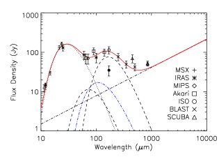
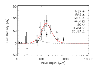
Figure 5.— Global SED of the Cas A SNR. A fit was made to published MSX, IRAS, and Spitzer/MIPS photometry (Hines et al., 2004) together with the new AKARI and BLAST and remeasured ISO 170 $\mu$m (open circle) data, but neither the original Tuffs et al. (1999) value (filled circle) nor the SCUBA data (triangles) were used. The model used for this fit is given in equation 3, and contains physically motivated components attributable to line of sight interstellar dust, and dust and synchrotron emission from the SNR. The two broad peaks in panel (a) are from hot SNR dust (dotted curve) and cold dust (upper dashed curve) with derived temperatures 99$\pm$3 K and 16.6$\pm$1.3 K, respectively. More minor components are the new tepid dust Gaussian component in the SNR (§ 3; dot-dash curve) and VSGs (lower dashed curve). These contribute in the spectrally-confused 100 $\mu$m region and cannot be separated using this global SED alone. For panel (b), the flux of the synchrotron and hot and tepid dust components have been subtracted to highlight the contribution of cold dust and, less importantly, VSGs.

In order to fit these data we developed a physically motivated model with four dust components as discussed above, including hot dust (subscript H), the tepid Gaussian component (G), cold dust (C), and VSGs (V), together with synchrotron emission, and described by:

$$S_{\nu}=\sum_{i=1,4}\Omega_{i}\nu^{\beta_{i}}B_{\nu}(T_{i})+S_{\rm{0}}(\nu/\nu_{\rm{0}})^{\alpha},$$ (3)

where the scale factors $\Omega$ are related to the spatially-integrated column density or mass. All four dust components have been approximated as single-temperature modified blackbodies. We obtain the synchrotron fluxes by extrapolation from the map of Wright et al. (1999) and subtract them from $S_{\nu}$ and so these data are not part of the fit to find the dust parameters.

For the cold dust (largely interstellar), we take $\beta_{\rm C}=2$ (Li and Draine, 2001) and find the other two parameters, $\Omega$ and $T$, from the fit.

The value of $\beta_{\rm{H}}$ is much less certain. Furthermore, this is a highly simplistic model, as the hot modified-blackbody underestimates the emission from polycyclic aromatic hydrocarbons (PAH) and short-wavelength SNR features seen by Rho et al. (2008). $\beta_{\rm{H}}=1$ might be a better approximation to broaden the model SED to accommodate the range of hot dust temperatures, but we take it to be 2 to better describe the longer wavelength emission near 100 $\mu$m (Figure 3). The hot dust emission from the SNR dominates the total flux emitted in the short wavelength region of the SED and so its characteristic temperature $T_{\rm{H}}$ is well determined, but discovering exactly how the SED extrapolates to longer wavelengths requires morphological information, and is not the focus here.

The single-temperature approximation is least appropriate for the non-equilibrium emission by VSGs which would have a range of temperatures, but this is not critical here since the VSG emission is relatively weak. To help constrain the model, we take a representative $T_{\rm{V}}=40$ K, $\beta_{\rm{V}}=2$, and $\Omega_{\rm{V}}/\Omega_{\rm{C}}=1.8\times 10^{-3}$ determined from the large scale interstellar regions of the maps (§ 5). Consistent with the integrated spectrum shown in Figure 1, this results in the peak of the VSG emission being about 14% of that of the cold dust.

We take the parameters of the Gaussian component from our study in § 3, where the flux at 100 $\mu$m, near the peak, is found to be 16 Jy and the SED is as shown in Figure 3.

Fitting the remaining parameters to the global spectrum, the total model spectrum and its components are plotted in Figure 5. The original ISO 170 $\mu$m point and the SCUBA data were not included in our fits. The ISO flux we measure is consistent with the new BLAST and AKARI data, as well as with previously published data at other wavelengths. This fit does not appear consistent with the SCUBA data at either 450 or 850 $\mu$m, with the BLAST 500 $\mu$m point being $\sim$40% (1.8$\sigma$) lower than the SCUBA 450 $\mu$m value. We cannot find any explanation for this disparity.

We find $T_{\rm{H}}=99\pm$3 K and $T_{\rm{C}}=16.6\pm$1.3 K. For the same $\kappa$ as adopted for the tepid dust (for lack of better constraints), the independent masses of hot and cold dust (if the latter were all at 3.4 kpc) are 0.003 and 10 M_⊙, respectively. The latter is the potential amount of cold dust associated with the SNR, significant background emission having been subtracted when carrying out the photometry. This limit, close to that estimated by Krause et al. (2004), illustrates just how difficult it is to separate out cold dust in the SNR, given a strong interstellar signal. This too needs to be addressed using morphological information. It is noting that when the newly measured ISO point is exclulded from the fit there is only a negligible effect, changing the derived parameters by less than 1-$\sigma$ as compared to a fit performed without this datum.

5. Component Separation

The photometry in Figure 5 benefits from greater spectral coverage to provide an improved measurement of the spectral energy distribution toward Cas A, but does not explicitly address whether that emission, particularly the cold dust, is line of sight interstellar emission or is intrinsic to the SNR. Here we exploit the six large area AKARI and BLAST maps over the region observed in common. The maps were convolved to a resolution of $1\farcm 9$ and re-gridded to the same pixelization to produce a coarse spectral “cube”. Using a multi-component model akin to equation 3 in § 4, an independent fit to the SED at each pixel in this cube is carried out and maps of each free parameter obtained.

We first subtracted the SNR synchrotron component from the data and so, as in § 4, this model component is not a part of the fit. We convolved the 83 GHz radio map of Wright et al. (1999) to produce a synchrotron template, and subtracted the appropriate intensity by extrapolating the spectrum assuming a power-law spectral index of $\alpha=-0.72$ (see § 2.3). This left us with maps containing only thermal dust emission, but still four components on the line of sight to the SNR, which introduces too many free parameters. Therefore, benefiting from the higher resolution analysis in § 3, we also subtract from the maps the tepid dust Gaussian component found there.

Because the analysis here uses only the AKARI and BLAST maps, it does not contain information from wavelengths shorter than 65 $\mu$m. Consequently it is not necessary or possible to have a sophisticated modeling of short wavelength emission sources (e.g., PAHs and shorter wavelength VSG emission). We simply used $T_{\rm{V}}=40$ K and $\beta_{\rm{V}}=2$ as above. Additionally, toward the SNR the intensity of the VSG component used in this simple model is degenerate with the hot dust ring component and tepid dust Gaussian component because of the overlapping SEDs, meaning that our analysis is not sensitive to whether the ratio of VSG to cold dust emission for putative SNR dust might be different than the equivalent ratio for the interstellar line of sight cloud. Away from the SNR we allowed this ratio to vary in order to examine its statistical properties, and then we adopted the average ratio for the confused line of sight to the SNR. The properties of the cold dust (column density and temperature) outside the SNR are quite similar whether this average ratio is used in the model for the whole map, or is allowed to be fit.

The hot dust component should only be included in the model for pixels where the SNR contributes to the intensity. In order to assess in an objective automated way whether or not the data to which the model is fit contain emission from the SNR, the AKARI 65 to 140 $\mu$m ratio was examined. A maximum ratio of 0.22 was found for all regions beyond a 4^′ radius from the SNR. Therefore, only when the ratio exceeded this value was this hot component included in the model fit. The temperature of the hot component is held fixed at 100 K, as derived in § 4 with $\beta_{\rm{H}}=2$, and its amplitude (column density) allowed to vary. As an alternative, we experimented with removing this emission component from the map using a scaled hot dust template. This final cleaning step was not entirely satisfactory, probably because of changes in the hot dust SED (temperature) across the face of the SNR, but again the derived properties of the cold dust were not very sensitive to this choice. As another sensitivity test, we fit using a hot dust model with $T_{\rm{H}}=120$ K and $\beta_{\rm{H}}=1$ and again the cold dust parameters were robust, because the overlap of the cold and hot SEDs is not great (Figure 5).

Our six-wavelength data are fit using a model which contains either two or three free parameters, depending on whether the data being fit contains a contribution from the SNR. These parameters are the hot dust amplitude, the cold dust amplitude, and the cold dust temperature, $T_{\rm{C}}$. Implicit in this is the assumption that the cold dust model component is sufficient to describe the emission from both the SNR and line of sight interstellar clouds. A reduced $\chi^{2}$ measurement was calculated for each pixel fit; the median value over the map was 0.89.

The output maps are presented in Figure 6, with contours from the radio synchrotron emission (Wright et al., 1999) overlaid to show the location and approximate size of the SNR.

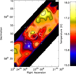
(a) Cold temperature

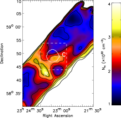
(b) Cold column density

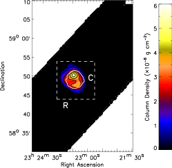
(c) Hot column density

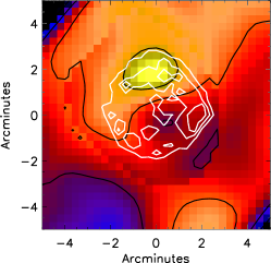
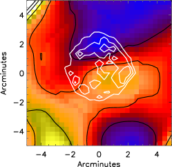
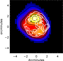
Figure 6.— Output maps for the three free parameters of the spectral model: temperature of the cold dust and column density of both cold and hot dust. In the upper panels a single white contour from the 83 GHz radio map (Wright et al., 1999) shows the approximate position of the Cas A SNR forward shock (Helder and Vink, 2008). The letters C and R label the elliptical line of sight “cloud” and “ridge” featured high-lighted in 2d respectively. The contour lines vary in steps of 0.5 K, $0.5\times 10^{22}$ cm^-2, and 1$\times$10^-8 g cm^-2 for maps a–c, respectively. Note that the outer edge regions are corrupted by convolution artifacts. The lower panels show magnified versions of the output within the white dashed square centered on $23^{h}23^{m}24^{s}$, $+58^{\circ}48^{\prime}54^{\prime\prime}$, overlaid with several white radio contours.

We find interstellar cloud temperatures ranging between 15 and 18 K, with a median of 16.5 K (see Figure 6a), in keeping with the temperature found by Wilson et al. (1993) and the cold dust temperature found by Dunne et al. (2003). The fine structure in this temperature map reflects some interplay between the various model components contributing to the emission model, but the main features there are robust against exactly how these spectral components are treated.

The Cas A SNR does not stand out particularly. There is a slightly hotter spot to the north of the SNR whose amplitude changes with the choice of alternative hot dust models and so probably reflects a deficiency there where the hot dust component is very bright. There is no telltale change in temperature at the location of Cas A, to indicate the presence of a significant secondary cold dust grain population at a different temperature to the interstellar cloud.

The cold component column density map (Figure 6b) shows distinctly the cold dust ridge (R) to the south-east of the SNR, and the cold elliptical region (C) to the west of and overlapping the SNR (the “line of sight cloud”).

Note that feature C is not as strong as R, is not obviously correlated with any morphological features of the SNR, and extends to the west beyond the remnant. The cold column density map resembles what is seen in integrated molecular line emission (Figure 7; see also Figure 4 of Liszt and Lucas 1999, Figure 1 of Krause et al. 2004, Figure 1 of Wilson and Batrla 2005, and Figure 8 of Dunne et al. 2009). Therefore we conclude that there is, by chance, a substantial amount of interstellar material projected on the Cas A line of sight. This makes it difficult to make a statistically significant detection of cold dust distinctly associated with the SNR with these data. It is likely that this confusion affected the measurements made by Dunne et al. (2003) based on chopped SCUBA observations. We can not identify the polarized dust source found by Dunne et al. (2009); however, based on our analysis of the data, this is to be expected as the flux density level predicted would be too faint to detect in our observations.

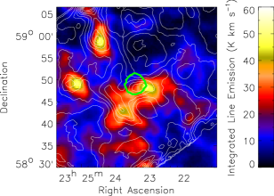
Figure 7.— Integrated ¹²CO ($1-0$) line emission from the FCRAO spectral cube in the CGPS (Taylor et al., 2003). Thin contours from the BLAST 250 $\mu$m map show the cold dust emission including the “line of sight cloud” and the “ridge” to the south-east. Thick contour indicates the position of the radio SNR as in Figure 6.

There is a large warmer-than-average region of $\sim$17 K to the north west which intersects with the remnant. Comparison with the column density map shows this to be part of a general anti-correlation between temperature and column density across the map. This could reflect a deficiency in the modeling, since the two are certainly inversely coupled, non-linearly, through equation 1. But it seems plausible that this has a physical origin. The high column density regions are molecular and, being more shielded from the interstellar radiation field which heats the dust, would be cooler. The low column density regions also tend to have a higher ratio of VSG emission, when this is allowed to vary in the fit, though this might be indicative of another effect as well, evolution of the grain size distribution.

The third output map, Figure 6c, shows the column density from the hot SNR dust component. The automated fitting has invoked this component only at the location of the SNR, the interstellar dust model being sufficient at locations away from the SNR. As expected, the structure of the emission is similar to that in the 65 $\mu$m band when convolved to the same resolution as the BLAST data.

Quantitatively, the hot and cold component amplitudes were converted to dust mass column density using equation 1. In principle different values of $\kappa_{\nu}$ would be used for the different dust components in different environments but, in the absence of persuasive evidence, we proceeded as in §§ 3-4 and adopted those of Li and Draine (2001) ($\kappa_{\rm{100}}=30\,{\rm cm^{2}g^{-1}}$; $\beta=2$) which are suitable for the diffuse ISM. Since much of the ISM in this region is in molecular form, these might not be entirely appropriate even for that component. The value of $\kappa_{\nu}$ represents the greatest uncertainty in this analysis, with published values spanning two orders of magnitude, depending on the dust type and environment (Dunne et al., 2003).

For the cold dust component, which is dominated by the line of sight interstellar dust, we further convert the dust mass column density into $N_{\rm{H}}$ by dividing by $1.9\times 10^{-26}\,{\rm g\,H^{-1}}$ (Li and Draine, 2001). $N_{\rm{H}}$, used in Figure 6b, is the metric quantifying X-ray photoelectric absorption, discussed in § 5.1. The column densities are large throughout the map, of order $10^{22}$ cm^-2. Similarly, this can in turn be converted to optical extinction $A_{\rm{V}}$ by dividing by $1.9\times 10^{21}\,{\rm cm^{-2}\,mag^{-1}}$ (Bohlin et al., 1978), equivalent to multiplying the mass column density directly by $2.8\times 10^{4}\,{\rm cm^{2}\,g^{-1}\,mag}$. The relationship between $N_{\rm{H}}$ and $A_{\rm{V}}$ is empirically calibrated only below about $N_{\rm{H}}=0.4\times 10^{22}\,{\rm cm^{-2}}$ or $A_{\rm{V}}=2$ (Kim and Martin, 1996) but might still be a reasonable approximation for the interstellar material spread out along this long line of sight.

Note that both $N_{\rm{H}}$ and $A_{\rm{V}}$, being scaled from estimates based on optically-thin submillimeter emission, measure the total column extending through the Galaxy. The column in the foreground of Cas A should be comparable to this, simply given the large distance to the SNR and Galactic latitude, $-2.1$^∘, and longitude, 111.7^∘. In fact, the velocity range of molecular lines seen in absorption against Cas A is the same as that seen in emission (§ 5.1) suggesting that Cas A is beyond most of the Perseus arm gas. Judging from the H I 21-cm emission-line spectrum along adjacent lines of sight in the CGPS data cube (Taylor et al., 2003), up to $0.1\times 10^{22}$ cm^-2 might be in the background, or less than 10%.

If the cold dust projected on the remnant were all at that distance, the mass column density integrated over its face in a 5^′ diameter aperture would amount to $\sim 40$ $M_{\odot}$. This is a few times larger than found in § 4 because here there has been no subtraction of a “background”; Figure 6b shows that the column density on surrounding interstellar lines of sight is substantial. Dunne et al. (2009) suggest detection of 1 $M_{\odot}$ in the SNR whereas Krause et al. (2004) find an upper limit of 0.2 $M_{\odot}$. One has to beware of the different $\kappa$ and $T_{\rm{C}}$ that have been adopted in different derivations (the latter was not well constrained previously). In any case, it is again clear that the line of sight interstellar emission is an overwhelming source of contamination, with the searched-for SNR signal at the few percent level. Identifying cold SNR dust will be challenging even with the improved resolution of Herschel working close to the peak of the cold dust emission.

5.1. Other Measures of Interstellar Column Density

A supplementary approach would be to look at other measures of the ISM column density as a surrogate for the morphology and brightness level expected for the contaminating interstellar dust emission.

One potential surrogate for column density is molecular line emission. Molecular emission is affected variously by optical depth, abundance, and excitation conditions, and so a precise one-to-one correspondence with dust emission would not be expected. Nevertheless, even Figure 7, the integrated line emission from the FCRAO ¹²CO ($1-0$) data cube in the CGPS (Taylor et al., 2003), looks remarkably similar, though not identical, to the cold dust emission over this extended region (Figures 2c–f) and to the column density map (Figures 6b and e). Near the SNR, the integrated CO ($2-1$) map by Liszt and Lucas (1999) also shows features recognizable in the dust emission, including the western peak and the separated south-east ridge. Wilson and Batrla (2005) emphasize how ¹³CO ($1-0$) also projects on the SNR. These tracers suggest, as does the larger CGPS map, that the dust emission from the interstellar cloud C should extend beyond the SNR to the west. Note also the molecular emission toward the center of the SNR in these maps. The correlation of dust emission and molecular emission is not and cannot be expected to be perfect, but it is clear that interstellar line of sight dust emission is a major contaminant.

If the interstellar material seen along the line of sight is substantially in the foreground of the Cas A SNR emission, as appears to be the case, then measures of absorption can be used to trace column density. There are three approaches: (i) molecular lines (OH: Bieging and Crutcher 1986; methanol: Reynoso and Goss 2002) and the H I 21-cm line (e.g., Keohane et al. 1996), (ii) optical reddening (Fesen et al., 2006b), and (iii) X-ray absorption (Keohane et al., 1998; Vink et al., 1999; Hughes et al., 2000; Willingale et al., 2002). These give qualitatively the same results: (i) the column density is highest toward the west of the SNR, where we see the residual at 100 and 140 $\mu$m after subtracting the tepid Gaussian component (§ 3), (ii) there are patchy enhancements along a band extending from the west to the south-east, thus covering the south-west and south portion of the remnant, like feature C in our cold column density map and the molecular emission, (iii) the absorption is lowest across the north-east, but (iv) there is a substantial column everywhere, including toward the center (and the neutron star), and (v) the surrogate column density is about the same as derived in the above component separation, which indicates that our choice of $\kappa_{\rm{100}}$ was reasonable.

Quantitatively, column densities from the extinction surrogates are of order $10^{22}\ {\rm cm}^{-2}$, in these units about 2.3 toward the western maximum and 1.3 toward the center ($A_{V}\sim 7$). Not only are these values and the low contrast in column density comparable to what we found independently above, but there is also morphological similarity. Compare, for example, Figure 1c in Keohane et al. (1996) and Figure 4 in Willingale et al. (2002) to our cold dust column density map in Figure 6e. This leaves little room for an additional contribution at long wavelengths from the Gaussian “tepid” SNR dust component or a colder one.

Krause et al. (2004) show that the patchy OH absorption correlates well with the residual 850 $\mu$m emission seen with SCUBA (after subtracting the synchrotron emission), and on subtracting this foreground emission (scaled using $T_{\rm{d}}=14$ K) from their 160 $\mu$m map they find only a small residual and hence the above-mentioned upper limit of 0.2 M_⊙ of cold dust associated with the SNR.

Accounting for and removal of the (foreground) emission by correlations with extinction or molecular emission does seem a promising technique. It will be interesting to see if it proves useful pixel by pixel with forthcoming high signal to noise data or only statistically. Clearly the higher resolution imaging anticipated with Herschel will be essential for making progress along these lines.

6. Conclusions

1. We presented far-infrared/submillimeter data at 65 – 500 $\mu$m for the Cas A supernova remnant and the surrounding region. We used these maps to characterize the interstellar dust emission using data from cloud regions well beyond the SNR.

2. We used high resolution ARAKI data to probe the spectral region between the hot dust emission from the SNR shock-front and cold dust emission. Using a spectrum-informed clean technique we identified a new tepid dust population at temperature of $\sim$35 K. The mass of this individual dust population was estimated to be 0.06 M$\odot$, but with considerable uncertainty because of its dependence on the choice of $\kappa$.

3. The dust yield for this new and independent tepid component is comparable to that estimated previously for the hot dust component by Rho et al. (2008). While such yields could contribute to the dust masses seen in high redshift galaxies, they are still less than the required level 0.4-1 M_⊙estimated by Dwek et al. (2007). While the mass we measure is insufficient to account for the dust observed at high redshift, when taken in combination with the hot and cold dust masses previously reported by Rho et al. (2008) and Dunne et al. (2009), it strengthens the argument for supernovae as a potentially significant source of dust production in the high-redshift universe.

4. We developed a simple physically-motivated model of the SED of the SNR and interstellar emission and fit this to six-wavelength bands at each pixel. From this we obtained temperature and dust mass column density maps. The interstellar dust was found to be at a temperature of $\sim 16.5$ K, in keeping with previous measurements, but now better constrained due to the improved wavelength coverage.

5. We show that the high level of confusion arising from the interstellar cloud structure projected on the SNR precludes a significant detection of cold dust directly associated with Cas A. The same source of confusion will have affected previous estimates of cold dust in Cas A, increasing the uncertainty of those estimates. This analysis was not sufficiently sensitive to identify the lower limiting mass found by Dunne et al. (2009) or the lower value by Krause et al. (2004) and therefore does not preclude the possibility of a significant population of cold SNR dust grains with temperature close to that of the interstellar dust. The higher angular resolution data anticipated with Herschel working close to the peak of the cold dust emission, together with correlations with surrogates of the interstellar column density, could result in a more sensitive probe.

References

- Archibald et al. (2001) Archibald, E. N., Dunlop, J. S., Hughes, D. H., Rawlings, S., Eales, S. A., and Ivison, R. J.: 2001, MNRAS 323, 417
- Arendt et al. (1999) Arendt, R. G., Dwek, E., and Moseley, S. H.: 1999, ApJ 521, 234
- Atoyan et al. (2000) Atoyan, A. M., Tuffs, R. J., Aharonian, F. A., and Völk, H. J.: 2000, A&A 354, 915
- Bieging and Crutcher (1986) Bieging, J. H. and Crutcher, R. M.: 1986, ApJ 310, 853
- Bohlin et al. (1978) Bohlin, R. C., Savage, B. D., and Drake, J. F.: 1978, ApJ 224, 132
- Clayton et al. (1999) Clayton, D. D., Liu, W., and Dalgarno, A.: 1999, Science 283, 1290
- Desert et al. (1990) Desert, F.-X., Boulanger, F., and Puget, J. L.: 1990, A&A 237, 215
- Dickel et al. (1988) Dickel, J. R., Sault, R., Arendt, R. G., Korista, K. T., and Matsui, Y.: 1988, ApJ 330, 254
- Draine (2003) Draine, B. T.: 2003, ARA&A 41, 241
- Dunlop et al. (1994) Dunlop, J. S., Hughes, D. H., Rawlings, S., Eales, S. A., and Ward, M. J.: 1994, Nature 370, 347
- Dunne et al. (2003) Dunne, L., Eales, S., Ivison, R., Morgan, H., and Edmunds, M.: 2003, Nature 424, 285
- Dunne et al. (2009) Dunne, L., Maddox, S. J., Ivison, R. J., Rudnick, L., Delaney, T. A., Matthews, B. C., Crowe, C. M., Gomez, H. L., Eales, S. A., and Dye, S.: 2009, MNRAS 394, 1307
- Dwek (2004) Dwek, E.: 2004, ApJ 607, 848
- Dwek et al. (2007) Dwek, E., Galliano, F., and Jones, A. P.: 2007, ApJ 662, 927
- Dwek et al. (1987) Dwek, E., Hauser, M. G., Dinerstein, H. L., Gillett, F. C., and Rice, W. L.: 1987, ApJ 315, 571
- Dwek and Werner (1981) Dwek, E. and Werner, M. W.: 1981, ApJ 248, 138
- Ennis et al. (2006) Ennis, J. A., Rudnick, L., Reach, W. T., Smith, J. D., Rho, J., DeLaney, T., Gomez, H., and Kozasa, T.: 2006, ApJ 652, 376
- Ercolano et al. (2007) Ercolano, B., Barlow, M. J., and Sugerman, B. E. K.: 2007, MNRAS 375, 753
- Fesen et al. (2006a) Fesen, R. A., Hammell, M. C., Morse, J., Chevalier, R. A., Borkowski, K. J., Dopita, M. A., Gerardy, C. L., Lawrence, S. S., Raymond, J. C., and van den Bergh, S.: 2006a, ApJ 645, 283
- Fesen et al. (2006b) Fesen, R. A., Pavlov, G. G., and Sanwal, D.: 2006b, ApJ 636, 848
- Helder and Vink (2008) Helder, E. A. and Vink, J.: 2008, ApJ 686, 1094
- Hines et al. (2004) Hines, D. C., Rieke, G. H., Gordon, K. D., Rho, J., Misselt, K. A., Woodward, C. E., Werner, M. W., Krause, O., Latter, W. B., Engelbracht, C. W., Egami, E., Kelly, D. M., Muzerolle, J., Stansberry, J. A., Su, K. Y. L., Morrison, J. E., Young, E. T., Noriega-Crespo, A., Padgett, D. L., Gehrz, R. D., Polomski, E., Beeman, J. W., and Haller, E. E.: 2004, ApJS 154, 290
- Holland et al. (1999) Holland, W. S., Robson, E. I., Gear, W. K., Cunningham, C. R., Lightfoot, J. F., Jenness, T., Ivison, R. J., Stevens, J. A., Ade, P. A. R., Griffin, M. J., Duncan, W. D., Murphy, J. A., and Naylor, D. A.: 1999, MNRAS 303, 659
- Houck et al. (2004) Houck, J. R., Roellig, T. L., Van Cleve, J., Forrest, W. J., Herter, T. L., Lawrence, C. R., Matthews, K., Reitsema, H. J., Soifer, B. T., Watson, D. M., Weedman, D., Huisjen, M., Troeltzsch, J. R., Barry, D. J., Bernard-Salas, J., Blacken, C., Brandl, B. R., Charmandaris, V., Devost, D., Gull, G. E., Hall, P., Henderson, C. P., Higdon, S. J. U., Pirger, B. E., Schoenwald, J., Sloan, G. C., Uchida, K. I., Appleton, P. N., Armus, L., Burgdorf, M. J., Fajardo-Acosta, S. B., Grillmair, C. J., Ingalls, J. G., Morris, P. W., and Teplitz, H. I.: 2004, in J. C. Mather (ed.), Society of Photo-Optical Instrumentation Engineers (SPIE) Conference Series, Vol. 5487 of Society of Photo-Optical Instrumentation Engineers (SPIE) Conference Series, pp 62–76
- Hughes (1999) Hughes, J. P.: 1999, ApJ 527, 298
- Hughes et al. (2000) Hughes, J. P., Rakowski, C. E., Burrows, D. N., and Slane, P. O.: 2000, ApJ 528, L109
- Isaak et al. (2002) Isaak, K. G., Priddey, R. S., McMahon, R. G., Omont, A., Peroux, C., Sharp, R. G., and Withington, S.: 2002, MNRAS 329, 149
- Kawada et al. (2007) Kawada, M., Baba, H., Barthel, P. D., Clements, D., Cohen, M., Doi, Y., Figueredo, E., Fujiwara, M., Goto, T., Hasegawa, S., Hibi, Y., Hirao, T., Hiromoto, N., Jeong, W.-S., Kaneda, H., Kawai, T., Kawamura, A., Kester, D., Kii, T., Kobayashi, H., Kwon, S. M., Lee, H. M., Makiuti, S., Matsuo, H., Matsuura, S., Müller, T. G., Murakami, N., Nagata, H., Nakagawa, T., Narita, M., Noda, M., Oh, S. H., Okada, Y., Okuda, H., Oliver, S., Ootsubo, T., Pak, S., Park, Y.-S., Pearson, C. P., Rowan-Robinson, M., Saito, T., Salama, A., Sato, S., Savage, R. S., Serjeant, S., Shibai, H., Shirahata, M., Sohn, J., Suzuki, T., Takagi, T., Takahashi, H., Thomson, M., Usui, F., Verdugo, E., Watabe, T., White, G. J., Wang, L., Yamamura, I., Yamauchi, C., and Yasuda, A.: 2007, PASJ 59, 389
- Keohane et al. (1998) Keohane, J. W., Gotthelf, E. V., and Petre, R.: 1998, ApJ 503, L175+
- Keohane et al. (1996) Keohane, J. W., Rudnick, L., and Anderson, M. C.: 1996, ApJ 466, 309
- Kessler et al. (1996) Kessler, M. F., Steinz, J. A., Anderegg, M. E., Clavel, J., Drechsel, G., Estaria, P., Faelker, J., Riedinger, J. R., Robson, A., Taylor, B. G., and Ximenez de Ferran, S.: 1996, A&A 315, L27
- Kim and Martin (1996) Kim, S.-H. and Martin, P. G.: 1996, ApJ 462, 296
- Kozasa et al. (1991) Kozasa, T., Hasegawa, H., and Nomoto, K.: 1991, A&A 249, 474
- Krause et al. (2004) Krause, O., Birkmann, S. M., Rieke, G. H., Lemke, D., Klaas, U., Hines, D. C., and Gordon, K. D.: 2004, Nature 432, 596
- Krause et al. (2008) Krause, O., Birkmann, S. M., Usuda, T., Hattori, T., Goto, M., Rieke, G. H., and Misselt, K. A.: 2008, Science 320, 1195
- Lagage et al. (1996) Lagage, P. O., Claret, A., Ballet, J., Boulanger, F., Cesarsky, C. J., Cesarsky, D., Fransson, C., and Pollock, A.: 1996, A&A 315, L273
- Li and Draine (2001) Li, A. and Draine, B. T.: 2001, ApJ 554, 778
- Liszt and Lucas (1999) Liszt, H. and Lucas, R.: 1999, A&A 347, 258
- Meikle et al. (2007) Meikle, W. P. S., Mattila, S., Pastorello, A., Gerardy, C. L., Kotak, R., Sollerman, J., Van Dyk, S. D., Farrah, D., Filippenko, A. V., Höflich, P., Lundqvist, P., Pozzo, M., and Wheeler, J. C.: 2007, ApJ 665, 608
- Mezger et al. (1986) Mezger, P. G., Tuffs, R. J., Chini, R., Kreysa, E., and Gemuend, H.-P.: 1986, A&A 167, 145
- Morgan et al. (2003) Morgan, H. L., Dunne, L., Eales, S. A., Ivison, R. J., and Edmunds, M. G.: 2003, ApJ 597, L33
- Morgan and Edmunds (2003) Morgan, H. L. and Edmunds, M. G.: 2003, MNRAS 343, 427
- Neugebauer et al. (1984) Neugebauer, G., Habing, H. J., van Duinen, R., Aumann, H. H., Baud, B., Beichman, C. A., Beintema, D. A., Boggess, N., Clegg, P. E., de Jong, T., Emerson, J. P., Gautier, T. N., Gillett, F. C., Harris, S., Hauser, M. G., Houck, J. R., Jennings, R. E., Low, F. J., Marsden, P. L., Miley, G., Olnon, F. M., Pottasch, S. R., Raimond, E., Rowan-Robinson, M., Soifer, B. T., Walker, R. G., Wesselius, P. R., and Young, E.: 1984, ApJ 278, L1
- Pascale et al. (2008) Pascale, E., Ade, P. A. R., Bock, J. J., Chapin, E. L., Chung, J., Devlin, M. J., Dicker, S., Griffin, M., Gundersen, J. O., Halpern, M., Hargrave, P. C., Hughes, D. H., Klein, J., MacTavish, C. J., Marsden, G., Martin, P. G., Martin, T. G., Mauskopf, P., Netterfield, C. B., Olmi, L., Patanchon, G., Rex, M., Scott, D., Semisch, C., Thomas, N., Truch, M. D. P., Tucker, C., Tucker, G. S., Viero, M. P., and Wiebe, D. V.: 2008, ApJ 681, 400
- Patanchon et al. (2008) Patanchon, G., Ade, P. A. R., Bock, J. J., Chapin, E. L., Devlin, M. J., Dicker, S., Griffin, M., Gundersen, J. O., Halpern, M., Hargrave, P. C., Hughes, D. H., Klein, J., Marsden, G., Martin, P. G., Mauskopf, P., Netterfield, C. B., Olmi, L., Pascale, E., Rex, M., Scott, D., Semisch, C., Truch, M. D. P., Tucker, C., Tucker, G. S., Viero, M. P., and Wiebe, D. V.: 2008, ApJ 681, 708
- Pérez-Rendón et al. (2002) Pérez-Rendón, B., García-Segura, G., and Langer, N.: 2002, in W. J. Henney, J. Franco, and M. Martos (eds.), Revista Mexicana de Astronomia y Astrofisica Conference Series, pp 94–94
- Priddey et al. (2008) Priddey, R. S., Ivison, R. J., and Isaak, K. G.: 2008, MNRAS 383, 289
- Raymond (1984) Raymond, J. C.: 1984, ARA&A 22, 75
- Reed et al. (1995) Reed, J. E., Hester, J. J., Fabian, A. C., and Winkler, P. F.: 1995, ApJ 440, 706
- Reynoso and Goss (2002) Reynoso, E. M. and Goss, W. M.: 2002, ApJ 575, 871
- Rho et al. (2008) Rho, J., Kozasa, T., Reach, W. T., Smith, J. D., Rudnick, L., DeLaney, T., Ennis, J. A., Gomez, H., and Tappe, A.: 2008, ApJ 673, 271
- Rho et al. (2003) Rho, J., Reynolds, S. P., Reach, W. T., Jarrett, T. H., Allen, G. E., and Wilson, J. C.: 2003, ApJ 592, 299
- Rieke et al. (2004) Rieke, G. H., Young, E. T., Cadien, J., Engelbracht, C. W., Gordon, K. D., Kelly, D. M., Low, F. J., Misselt, K. A., Morrison, J. E., Muzerolle, J., Rivlis, G., Stansberry, J. A., Beeman, J. W., Haller, E. E., Frayer, D. T., Latter, W. B., Noriega-Crespo, A., Padgett, D. L., Hines, D. C., Bean, J. D., Burmester, W., Heim, G. B., Glenn, T., Ordonez, R., Schwenker, J. P., Siewert, S., Strecker, D. W., Tennant, S., Troeltzsch, J. R., Unruh, B., Warden, R. M., Ade, P. A., Alonso-Herrero, A., Blaylock, M., Dole, H., Egami, E., Hinz, J. L., LeFloch, E., Papovich, C., Perez-Gonzalez, P. G., Rieke, M. J., Smith, P. S., Su, K. Y. L., Bennett, L., Henderson, D., Lu, N., Masci, F. J., Pesenson, M., Rebull, L., Rho, J., Keene, J., Stolovy, S., Wachter, S., Wheaton, W., Richards, P. L., Garner, H. W., Hegge, M., Henderson, M. L., MacFeely, K. I., Michika, D., Miller, C. D., Neitenbach, M., Winghart, J., Woodruff, R., Arens, E., Beichman, C. A., Gaalema, S. D., Gautier, III, T. N., Lada, C. J., Mould, J., Neugebauer, G. X., and Stapelfeldt, K. R.: 2004, in J. C. Mather (ed.), Society of Photo-Optical Instrumentation Engineers (SPIE) Conference Series, Vol. 5487 of Society of Photo-Optical Instrumentation Engineers (SPIE) Conference Series, pp 50–61
- Silverberg et al. (1993) Silverberg, R. F., Hauser, M. G., Boggess, N. W., Kelsall, T. J., Moseley, S. H., and Murdock, T. L.: 1993, in M. S. Scholl (ed.), Society of Photo-Optical Instrumentation Engineers (SPIE) Conference Series, Vol. 2019 of Society of Photo-Optical Instrumentation Engineers (SPIE) Conference Series, pp 180–189
- Smith et al. (2009) Smith, J. D. T., Rudnick, L., Delaney, T., Rho, J., Gomez, H., Kozasa, T., Reach, W., and Isensee, K.: 2009, ApJ 693, 713
- Stickel et al. (2007) Stickel, M., Krause, O., Klaas, U., and Lemke, D.: 2007, A&A 466, 1205
- Taylor et al. (2003) Taylor, A. R., Gibson, S. J., Peracaula, M., Martin, P. G., Landecker, T. L., Brunt, C. M., Dewdney, P. E., Dougherty, S. M., Gray, A. D., Higgs, L. A., Kerton, C. R., Knee, L. B. G., Kothes, R., Purton, C. R., Uyaniker, B., Wallace, B. J., Willis, A. G., and Durand, D.: 2003, AJ 125, 3145
- Thorstensen et al. (2001) Thorstensen, J. R., Fesen, R. A., and van den Bergh, S.: 2001, AJ 122, 297
- Todini and Ferrara (2001) Todini, P. and Ferrara, A.: 2001, MNRAS 325, 726
- Truch et al. (2008) Truch, M. D. P., Ade, P. A. R., Bock, J. J., Chapin, E. L., Devlin, M. J., Dicker, S., Griffin, M., Gundersen, J. O., Halpern, M., Hargrave, P. C., Hughes, D. H., Klein, J., Marsden, G., Martin, P. G., Mauskopf, P., Netterfield, C. B., Olmi, L., Pascale, E., Patanchon, G., Rex, M., Scott, D., Semisch, C., Tucker, C., Tucker, G. S., Viero, M. P., and Wiebe, D. V.: 2008, ApJ 681, 415
- Tuffs et al. (1999) Tuffs, R. J., Fischera, J., Drury, L. O., Gabriel, C., Heinrichsen, I., Rasmussen, I., and Volk, H. J.: 1999, in P. Cox and M. Kessler (eds.), The Universe as Seen by ISO, Vol. 427 of ESA Special Publication, pp 241–+
- Tuffs et al. (2005) Tuffs, R. J., Popescu, C. C., and Voelk, H. J.: 2005, in Bulletin of the American Astronomical Society, Vol. 37 of Bulletin of the American Astronomical Society, pp 498–+
- Verdugo et al. (2007) Verdugo, E., Yamamura, I., and Pearson, C. P.: 2007, in AKARI FIS Data User Manual Version 1.3
- Vink et al. (1999) Vink, J., Maccarone, M. C., Kaastra, J. S., Mineo, T., Bleeker, J. A. M., Preite-Martinez, A., and Bloemen, H.: 1999, A&A 344, 289
- Werner (2006) Werner, M. W.: 2006, in Space Telescopes and Instrumentation I: Optical, Infrared, and Millimeter. Edited by Mather, John C.; MacEwen, Howard A.; de Graauw, Mattheus W. M.. Proceedings of the SPIE, Volume 6265, pp. (2006).
- Willingale et al. (2002) Willingale, R., Bleeker, J. A. M., van der Heyden, K. J., Kaastra, J. S., and Vink, J.: 2002, A&A 381, 1039
- Wilson and Batrla (2005) Wilson, T. L. and Batrla, W.: 2005, A&A 430, 561
- Wilson et al. (1993) Wilson, T. L., Mauersberger, R., Muders, D., Przewodnik, A., and Olano, C. A.: 1993, A&A 280, 221
- Woosley and Weaver (1995) Woosley, S. E. and Weaver, T. A.: 1995, ApJS 101, 181
- Wright et al. (1999) Wright, M., Dickel, J., Koralesky, B., and Rudnick, L.: 1999, ApJ 518, 284