Sub-Riemannian and sub-Lorentzian geometry on $\operatorname{SU}(1,1)$ and on its universal cover

Abstract.

We study sub-Riemannian and sub-Lorentzian geometry on the Lie group $\operatorname{SU}(1,1)$ and on its universal cover $\operatorname{\mathaccent 869{SU}}(1,1)$. In the sub-Riemannian case we find the distance function and completely describe sub-Riemannian geodesics on both $\operatorname{SU}(1,1)$ and $\operatorname{\mathaccent 869{SU}}(1,1)$, connecting two fixed points. In particular, we prove that there is a strong connection between the conjugate loci and the number of geodesics. In the sub-Lorentzian case, we describe the geodesics connecting two points on $\operatorname{\mathaccent 869{SU}}(1,1)$, and compare them with Lorentzian ones. It turns out that the reachable sets for Lorentzian and sub-Lorentzian normal geodesics intersect but are not included one to the other. A description of the timelike future is obtained and compared in the Lorentzian and sub-Lorentzain cases.

Contents

1. Introduction.

2. Sub-Riemannian and sub-Lorentzian geometry.

2.1. Sub-Riemannian manifolds.

2.2. Sub-Lorentzian manifolds.

2.3. Minimizing and maximizing curves seen from the viewpoint of optimal control.

3. Structure of the Lie groups $\operatorname{SU}(1,1)$ and $\operatorname{\mathaccent 869{SU}}(1,1)$.

3.1. Some notations.

3.2. Lie group $\operatorname{SU}(1,1)$.

3.3. Lie group structure of the universal cover $\operatorname{\mathaccent 869{SU}}(1,1)$ of $\operatorname{SU}(1,1)$.

4. Sub-Riemannian geometry on $\operatorname{SU}(1,1)$ and $\operatorname{\mathaccent 869{SU}}(1,1)$.

4.1. Geodesics, horizontal space, and vertical space.

4.2. Length and number of geodesics.

4.3. The cut and conjugate loci.

5. Sub-Lorentzian geometry on $\operatorname{\mathaccent 869{SU}}(1,1)$.

5.1. Sub-Lorentzian maximizers and geodesics on $\operatorname{\mathaccent 869{SU}}(1,1)$.

5.2. Number of geodesics.

5.3. Lorentzian and sub-Lorentzian timelike future.

6. Proofs of main results.

6.1. Proof of Proposition 2.

6.2. Proof of Corollary 1.

6.3. Proof of Proposition 5.

1. Introduction

Sub-Riemannian geometry is proved to play an important role in many applications, e.g., in mathematical physics and control theory. Sub-Riemannian geometry enjoys major differences from the Riemannian being a generalization of the latter at the same time, e.g., geodesics may be singular, the Hausdorff dimension is larger than the manifold topological dimension, the exponential map is never a local diffeomorphism. There exists a large amount of literature developing sub-Riemannian geometry. Typical general references are [17, 19, 20]. The sub-Lorentzian case is less studied and the first works in this directions appeared rather recenlty, see [8, 11, 12, 15].

In the development of sub-Riemannian geometry, one observes several examples, which are mainly nilpotent Lie groups, with either a left or right invariant distribution and metric. A sample representative is the Heisenberg group (see, e.g., [17]). Analysis of these groups in the sub-Riemannian setting, is already well studied. While these groups enjoy the advantage that explicit results are easier to obtain, their properties are sometimes too nice to be good examples to reveal all specific features of sub-Riemannian geometry in its generality. For instance, the cut locus and the conjugate loci for the Heisenberg group globally coincide.

A natural next step after considering nilpotent groups is to consider semisimple Lie groups. Let $G$ be such a group with the Lie algebra $\mathfrak{g}$. Let $\iota:\mathfrak{g}\rightarrow\mathfrak{g}$ be a Cartan involution (ex. for matrix algebras we can define $\iota$ as the map that sends an element $X$ to minus its conjugate transpose). Then there is a splitting $\mathfrak{g}=\mathfrak{k}\oplus\mathfrak{p}$, where $\mathfrak{k}$ and $\mathfrak{p}$ are the $+1$ and $-1$ eigenspaces of $\iota$. Remember that the Killing form

$$\mathrm{Kil}(X_{1},X_{2})=\mathrm{trace}(\mathrm{ad}_{X_{1}}\circ\mathrm{ad}_{X_{2}}),\qquad X_{1},X_{2}\in\mathfrak{g},$$

is non-degenerate when $\mathfrak{g}$ is semisimple. If $G$ is compact (or more generally, if $G/\mathcal{Z}(G)$ is compact, where $\mathcal{Z}(G)$ denotes the center of $G$), then $\mathfrak{g}=\mathfrak{k}$, and $-\mathrm{Kil}(\cdot,\cdot)$, is positive definite on $\mathfrak{g}$. So, we can use it to define a bi-invariant Riemannian metric on $G$. The restriction of this metric to a distribution on $G$ gives a sub-Riemannian manifold. An example of such manifold, $\operatorname{SU}(2)$ (or $S^{3}$ considered as the set of unit quaternions), was considered in [6, 9]. The problem of geodesic connectivity on $S^{3}$ was addressed in [9].

If $G$ is non-compact and $\mathfrak{p}\neq 0$ (i.e., $G/\mathcal{Z}(G)$ is non-compact), then the Killing form restricted to $\mathfrak{p}$ is positive definite. We consider a left translation of $\mathfrak{p}$ as our horizontal distribution, and using the metric induced by the Killing form, we obtain a sub-Riemannian manifold equipped with a bi-invariant metric. Let $K$ be a subgroup of $G$ with the Lie algebra $\mathfrak{k}$. Then $G$ is diffeomorphic to $K\times\mathfrak{p}$, by $(k,X)\mapsto ke^{X}$, and if $G$ has a finite center, then $K$ is a maximal compact subgroup. In addition, the above mentioned distribution is horizontal with respect to the quotient map

$$G\rightarrow G/K.$$

It follows that all normal geodesics are liftings of geodesics from $G/K$, hence they are of the form

$$t\mapsto g_{0}e^{tX}e^{-\operatorname{pr}_{\mathfrak{k}}tX},\qquad X\in\mathfrak{g},$$

where $g_{0}\in G$ is the initial point and $\operatorname{pr}_{\mathfrak{k}}:\mathfrak{g}\to\mathfrak{k}$ is the projection.

Here we consider an example with $G=\operatorname{SU}(1,1)$ and $K=\mathrm{U}(1)$. Although non-holonomic geometry on $\operatorname{SU}(1,1)$ (or the isometric case of $\operatorname{SL}(2)$) was first considered earlier in, e.g., [5, 21], we will obtain new results and a more complete description of geodesics both in sub-Riemannian and sub-Lorentzian settings. Much of all meaningful results come from the analysis of the universal cover of $\operatorname{SU}(1,1)$, which we denote by $\operatorname{\mathaccent 869{SU}}(1,1)$, and which is of its own interest as a new representative of a non-nilpotent Lie group over the topological space $\mathbb{R}^{3}$. We remark also that the Kähler manifold $\operatorname{SU}(1,1)/\operatorname{U}(1)$, is of particular importance in quantum field theories describing black holes in two-dimensional spacetime by means of an $\operatorname{SU}(1,1)/\operatorname{U}(1)$-gauged Wess-Zumino-Novikov-Witten model, see e.g., [7, 22].

Let $\mathfrak{su}(1,1)$ be the Lie algebra of $\operatorname{SU}(1,1)$. When considered as a bilinear form on the entire $\mathfrak{su}(1,1)$, the Killing form is an index 1 pseudo-metric. Furthermore, the induced Lorentzian metric on the Lie group makes $\operatorname{SU}(1,1)$ isometric to what is called the anti-de Sitter space $\operatorname{AdS}_{3}$ in General Relativity. This makes it tempting to study sub-Lorentzian geometry on $\operatorname{SU}(1,1)$. Apart from the fact that the Hamiltonian approach was proposed in [8] to study sub-Lorentzian structures on $\operatorname{SU}(1,1)$, the authors are not aware of other concrete examples so far, where sub-Lorentzian geometry is studied on any other manifold different from the Heisenberg group [11, 12] or its extension to the $\mathbb{H}$-type Carnot groups [15].

The notion of distance in sub-Lorentzian geometry, as well as in Lorentzian geometry, is given by the supremum of length over timelike curves. Since timelike loops may appear in $\operatorname{SU}(1,1)$, the distance function behaves badly (more specifically the distance from a point to itself is $\infty$). Therefore, sub-Lorentzian geometry on $\operatorname{\mathaccent 869{SU}}(1,1)$ is more interesting and meaningful than on $\operatorname{SU}(1,1)$. We are also interested in comparison of sub-Lorentzian and Lorentzian geometries on $\operatorname{\mathaccent 869{SU}}(1,1)$, in order to understand somewhat more, how the geometry changes when the Lorentzian metric is being restricted to a distribution. The strong interplay between $\operatorname{\mathaccent 869{SU}}(1,1)$ and $\operatorname{SU}(1,1)$ will, however, be practical for all explicit calculations.

The structure of the paper is as follows. Section 2 is devoted to general definitions and relations between sub-Riemannian and sub-Lorentzian geometry, and optimal control. Section 3 describes the Lie groups $\operatorname{SU}(1,1)$ and $\operatorname{\mathaccent 869{SU}}(1,1)$. Section 4 contains results concerning sub-Riemannnian geometry. We describe the number of geodesics connecting two points and give explicit formulas for the distance functions. The cut and conjugate loci on both Lie groups are given. We discuss the connection between the conjugate locus and the behavior of the geodesics. In section 5, we completely describe the two-point connectivity problem by sub-Lorentzian geodesics, and compare it with the Lorentzian case. The Lorentzian and sub-Lorentzian future for $\operatorname{\mathaccent 869{SU}}(1,1)$ are compared. It turns out that the reachable sets for Lorentzian and sub-Lorentzian normal geodesics intersect but are not included one to the other. Section 6 contains the proofs of main results.

The authors express special thanks to Mauricio Godoy and Irina Markina for many interesting discussions during seminars at the University of Bergen.

2. Sub Riemannian and Sub-Lorentzian geometry

2.1. Sub-Riemannian manifolds

A sub-Riemannian manifold is an $n$-dimensional manifold $M$, with a fiber metric $\rho$ on an $m$-dimensional smooth distribution $D\rightarrow M$ ($2\leq m\leq n$). By distribution, we mean a sub-bundle of the tangent bundle. Absolutely continuous curves that are almost everywhere tangent to $D$ are called horizontal. The length of a horizontal curve $\gamma:[0,\tau]\rightarrow M$, is defined by

$$\ell(\gamma):=\int_{0}^{\tau}\rho^{1/2}(\dot{\gamma}(t),\dot{\gamma}(t))\,dt.$$

The Carnot-Carathéodory distance between points $q_{0},q_{1}\in M$ is defined as

$$d(q_{0};q_{1})=\inf\limits_{\gamma}\ell(\gamma),$$

where the infimum is taken over all horizontal curves $\gamma$ satisfying $\gamma(0)=q_{0}$ and $\gamma(\tau)=q_{1}$. If there are no such curves connecting $q_{0}$ and $q_{1}$, then the distance is $\infty$. If the minimum in the above relation is attained, then the curve is called a length minimizing curve.

Define $D^{1}=D$ and iteratively $D^{i}=D^{i-1}+[D,D^{i-1}]$, $i\geq 2$, where $[\cdot,\cdot]$ denotes the Lie brackets, $[X,Y]=XY-YX$ for $X,Y\in T_{q}M$, $q\in M$. If there exists a positive integer $k\geq 2$, such that $D^{k}=TM$, then the distribution is called bracket generating. It is called regular if $\dim D^{i}_{q}$ is independent of the choice of $q$ for all $i$. We say that $D$ is step $k$ regular, if it is regular and $k$ is the smallest number for which $D^{k}=TM$. The Chow-Rashevskiĭ theorem [18, 10] states that a bracket generating distribution $D$ guarantees that any two points of $M$ may be connected by a horizontal curve. In addition, we have the following generalizations of the corresponding properties from the Riemannian case.

Theorem 1 (Hopf-Rinow theorem for sub-Riemannian manifolds [3]).

Suppose that $D$ satisfies the bracket generating condition. Then,

• any $q_{0}\in M$ has a neighborhood $U$, such that there exists a minimizing curve joining the points $q_{1}$ and $q_{0}$ for every $q_{1}\in U$;

• if $M$ is complete regarding to $d$, then any two points can be joined by a minimizing curve.

Observe, that the length minimizing curve may be singular for arbitrarily close points (see [16]).

A curve is called geodesic if it is locally a length minimizer. By a normal geodesic in the sub-Riemannian case we mean an integral curve of the Hamiltonian system generated by a Hamiltonian function $H=\sum_{j=1}^{m}h_{j}^{2}$ in some neighborhood of a point $q$ with respect to any local orthonormal basis $\{X_{1},\dots,X_{m}\}$ in this neighborhood. Here, and in rest of the paper, if $X$ is a vector field, then $h_{X}:T^{*}M\rightarrow\mathbb{R}$ denotes the Hamiltonian function

$$h_{X}:\lambda\mapsto\lambda(X(q)),\qquad\lambda\in T_{q}^{*}M,$$

with respect to the vector field $X$. If we have a basis $\{X_{1},\dots,X_{n}\}$, then we simplify notations by writing $h_{j}$ instead of $h_{X_{j}}$. One of the principal differences between sub-Riemannian and Riemannian geometries is that the function $q\mapsto d(q_{0};q)$ is not differentiable in any neighborhood of $q_{0}$ when $m<n$.

2.2. Sub-Lorentzian manifolds

A sub-Lorentzian manifold is defined similarly to a sub-Riemannian manifold, but with $\rho$ now being an index 1 pseudo-metric on $D$. We will say that a vector $v\in D$ is

• timelike if $\rho(v,v)<0$,

• lightlike or null if $\rho(v,v)=0$,

• spacelike if $\rho(v,v)>0$,

• causal or nonspacelike if $\rho(v,v)\leq 0$.

A chosen vector field $T$ in $D$, is said to be the time-orientation on $M$, if $\rho(T(q),T(q))<0$ for any $q\in M$. A causal vector $v$ is called future directed if $\rho(T(q),v)<0$, and past directed if $\rho(T(q),v)>0$. A horizontal curve $\gamma:[0,\tau]\ \rightarrow\mathbb{R}$ is called timelike, null, spacelike, causal, future directed or past directed, respectively, if $\dot{\gamma}(t)$ is such a vector for almost every $t\in[0,\tau]$. We define the timelike future $\mathcal{I}^{+}(q_{0},\rho)$ of $q_{0}$ with respect to $\rho$ as the set of all points $q_{1}\in M$, such that there is a horizontal, timelike future directed curve $\gamma$, with $\gamma(0)=q_{0}$ and $\gamma(\tau)=q_{1}$. The causal future, $\mathcal{J}^{+}(q_{0},\rho)$, is defined similarly, with timelikeness interchanged with causality. Analogous definitions are valid for the timelike or causal past, which we denote by $\mathcal{I}^{-}(q_{0},\rho)$ and $\mathcal{J}^{-}(q_{0},\rho)$ respectively. We define the length of a horizontal causal curve by $\ell(\gamma)=\int_{0}^{\tau}|\rho(\dot{\gamma}(t),\dot{\gamma}(t))|^{1/2}dt$. The sub-Lorentzian distance is defined by

$$d(q_{0};q_{1})=\left\{\begin{array}[]{ll}\sup\limits_{\gamma}\ell(\gamma),&\text{if \,}q_{1}\in\mathcal{J}^{+}(q_{0},\rho),\\ 0,&\text{otherwise}.\end{array}\right.$$

The supremum is taken over all horizontal future directed causal curves from $q_{0}$ to $q_{1}$. Similarly to the Lorentzian distance, the sub-Lorentzian distance satisfies the reverse triangle inequality, and may not be very well behaving. For instance, if there is a timelike loop trough a point $q\in M$, then $d(q;q)=\infty$.

A curve $\gamma:[0,\tau]\rightarrow\mathbb{R}$ is called a length maximizer, if $\ell(\gamma)=d(\gamma(0);\gamma(\tau))$. Similarly, a curve $\gamma$ is called a relative maximizer with respect to an open set $W$, if $\gamma([0,\tau])\subseteq W$ and $\ell(\gamma)=\sup_{\tilde{\gamma}}\ell(\tilde{\gamma})$, where the supremum is taken over all horizontal future directed causal curves contained in $W$, connecting $\gamma(0)$ and $\gamma(\tau)$. By using the maximum principle, for $D$ bracket generating, we know that all relative maximizers are either normal geodesics or strictly abnormal maximizers [12], and that the relative maximizers always exist locally. By normal sub-Lorentzian geodesics $\gamma$ we mean curves, such that for any local orthonormal basis $\{X_{1},\dots,X_{m}\}$ of $D$, with $X_{1}$ as the time-orientation, $\gamma$ is an integral curve of the Hamiltonian system generated by a Hamiltonian function $-h_{1}^{2}+\sum_{j=2}^{m}h_{j}^{2}$.

The question of whether length maximizers exist between two points, is a much more complicated than the question of the existence of length minimizers in Riemannian or sub-Riemannian geometries. The most common sufficient condition for the global existence of maximizing curves on a Lorentzian or sub-Lorentzian manifold $M$ is a relatively strict requirement that $M$ should be globally hyperbolic, i.e., strongly causal (every point has an arbitrarily small neighborhood, such that causal curves that leave the neighborhood never return back), and that $\mathcal{J}^{+}(q_{1},\rho)\cap\mathcal{J}^{-}(q_{2},\rho)$ is compact for any $q_{1},q_{2}\in M$.

2.3. Minimizing and maximizing curves seen from the viewpoint of optimal control

Determination of curves whose length is equal to the distance, either in the sub-Riemannian or sub-Lorentzian setting, can be formulated as a solution to an optimal control problem. Let $M$ be an $n$-dimensional manifold, let a submersion $\pi:\,V\rightarrow M$ be a fiber bundle with the fiber $U=\pi^{-1}(q)$, $q\in M$, and let $f:V\rightarrow TM$ be a fiber preserving map.

An admissible pair $v=(u,\gamma_{u})$ is a bounded measurable mapping $v:[0,\tau]\rightarrow V,0<\tau<\infty$ such that $\gamma_{u}=\pi\circ v$ is a Lipschitzian curve on $M$ and $\dot{\gamma}_{u}=f(u,\gamma_{u})$. The component $u$ is called control in the literature. For some fixed value of $\tau$, we denote the space of all admissible pairs by $\mathcal{V}_{\tau}$. The space $\mathcal{V}_{\tau}$ is a smooth Banach submanifold of $L^{\infty}([0,\tau],V)$, which is modeled on $L^{\infty}([0,\tau],\mathbb{R}^{\dim V})$. An admissible pair is said to connect $q_{0},q_{1}\in M$, if $\gamma_{u}(0)=q_{0}$, $\gamma_{u}(\tau)=q_{1}$. Such a system is called controllable, if any two points in $M$ are connected by at least one admissible pair. Let $J:\mathcal{V}_{\tau}\rightarrow\mathbb{R}$ be a functional, given by

$$J(v)=\int_{0}^{\tau}\mathcal{K}(v)dt\,,$$

where $\mathcal{K}$ is some differentiable function. Suppose we are given two points $q_{0},q_{1}\in M$, such that there is at least one admissible pair connecting them. An optimal control problem with respect to the functional $J$, is a problem of finding an element $v^{*}=(u^{*},\gamma_{u^{*}})\in\mathcal{V}_{\tau}$ connecting $q_{0},q_{1}$, such that for any $v\in\mathcal{V}_{\tau}$ connecting the same two points, we have $J(v^{*})\leq J(v)$. Analogously, we may look for the maximum of $J$. We call $u^{*}$ the optimal control, and $\gamma_{u^{*}}$ the optimal trajectory. We may also consider free-time optimal control problems where $\tau$ is allowed to vary.

We will write $\vec{H}$ to denote the Hamiltonian vector field associated to a Hamiltonian function $H$. For a pseudo-Hamiltonian function $\mathscr{H}$, the vector field $\vec{\mathscr{H}}$ is defined so that for a fixed $u\in U$, $\vec{\mathscr{H}}(u,\cdot)$ is the Hamiltonian vector field associated with $\mathscr{H}(u,\cdot)$. The main tool to solve optimal control problems is the following first order condition known as the Pontryagin Maximum Principle (PMP).

Theorem 2 (PMP for Optimal Control Problem with fixed time $\tau$).

For a given value of $\tau$, let $v^{*}=(u^{*},\gamma_{u^{*}})\in\mathcal{V}_{\tau}$ be an optimal pair for the above problem, i.e., $J(v^{*})=\min\limits_{v\in\mathcal{V}_{\tau}}\{J(v)\big{|}\,\gamma_{u}(0)=0,\gamma_{u}(\tau)=q_{1}\}$. For each $\varkappa\in\mathbb{R}$ a pseudo-Hamiltonian function $\mathscr{H}_{\varkappa}:\,U\times T^{*}M\to\mathbb{R}$ is defined by

$$\mathscr{H}_{\varkappa}(u,\lambda)=\lambda(f(u,q))+\varkappa\mathcal{K}(u,q),$$

where $\lambda\in T_{q}^{*}M$. Then there exists a curve $\xi:[0,\tau]\rightarrow T^{*}M$, and a number $\varkappa\leq 0$, such that

$$\dot{\xi}(t)=\vec{\mathscr{H}}_{\varkappa,}(u^{*},\xi(t)),\qquad\mathscr{H}_{\varkappa}(u^{*},\xi(t))=\max_{u\in U}\mathscr{H}_{\varkappa}(u,\xi(t))\quad\text{a.e. in}\,\,t\in[0,\tau],$$

and

$$\operatorname{pr}_{M}\xi(t)=\gamma_{u^{*}}(t).$$

The pseudo-Hamiltonian function is constant along the optimal trajectory $\xi(t)$. Moreover, if $\varkappa=0$, then for almost every $t\in[0,\tau]$, $\xi(t)$ can not be in the zero section of $T^{*}M$.

For the problem of the maximum of $J$, the above theorem has the same formulation, changing only the requirement $\varkappa\leq 0$ to $\varkappa\geq 0$. If we consider a free-time problem, then we also require $\mathscr{H}_{\varkappa}(u^{*},\xi(t))\equiv 0$ almost everywhere. If $\varkappa\neq 0$, then the solution is called normal (in this case we may just choose $\varkappa=\pm 1$). If $\varkappa=0$, the solution is called abnormal.

Remark 1 ([2]).

If $H_{\varkappa}(\lambda)=\max_{u\in U}\mathscr{H}_{\varkappa}(u,\lambda)$ is defined and is $C^{2}$ on $T^{*}M\setminus s_{0}(M)$, where $s_{0}:M\rightarrow T^{*}M$ is the zero-section, then $\dot{\xi}(t)=\vec{H}_{\varkappa}(\xi(t))$.

Let us turn to specific sub-Riemannian and sub-Lorentzian settings. We only need the formulation for the case when $M=G$ is a Lie group. This case is somewhat simpler since the tangent bundle of Lie groups is trivial, so we can always find a global basis to span a distribution. Let $D=\mathrm{span}\{X_{1},\dots,X_{m}\}$ be a distribution, and $\rho$ be either a sub-Riemannian or sub-Lorentzian metric on $D$. We may assume that the collection $\{X_{j}\}_{j=1}^{m}$ forms an orthonormal basis with respect to the metric $\rho$. Let $V=U\times G$, where $U\subset\mathbb{R}^{m}$. We choose $f(u_{1},\dots,u_{m},g)=u_{1}X_{1}(g)+\cdots+u_{m}X_{m}(g)$, $g\in G$, to ensure that $g(t)$ is a horizontal curve.

The determination of the sub-Riemannian distance, comes down to finding an optimal pair $(u^{*},g_{u^{*}}):[0,\tau]\rightarrow U\times G$ that minimizes the functional

$$J(u,g_{u})=\frac{1}{2}\int_{0}^{\tau}\sum_{j=1}^{m}u_{j}^{2}\,dt,\,\quad u\in U=\{u\in\mathbb{R}^{m}|\,\|u\|\leq 1\}.$$

The corresponding pseudo-Hamiltonian is given by

$$\mathscr{H}_{\varkappa}(u,\lambda)=-\frac{\varkappa}{2}\sum_{j=1}^{m}u_{j}^{2}+\sum_{j=1}^{m}u_{j}h_{j}(\lambda),\quad\lambda\in T^{*}G,\quad u\in U,\quad\varkappa=0,1.$$

As a consequence of Fillipov’s theorem [2], there always exists a length minimizing horizontal curve between two points in this setting.

Similarly, finding the sub-Lorentzian distance with $X_{1}$ as a time-orientation, means finding a pair $(u^{*},g_{u^{*}})$ that maximizes

$$J(u,g_{u})=\int_{0}^{\tau}\left(u_{1}^{2}-\sum_{j=2}^{m}u_{j}^{2}\right)^{\frac{1}{2}}\,dt,\quad\qquad U=\left\{u\in\mathbb{R}^{m}\big{|}\,u_{1}=\left(1+\sum_{j=2}^{m}u_{j}^{2}\right)^{\frac{1}{2}}\right\},$$

and the pseudo-Hamiltonian related to this problem becomes

$$\mathscr{H}_{\varkappa}(u,\lambda)=\varkappa\left(u_{1}^{2}-\sum_{j=2}^{m}u_{j}^{2}\right)^{\frac{1}{2}}+\sum_{j=1}^{m}u_{j}h_{j}(\lambda).$$

The latter case is more complicated because we optimize a non-convex functional.

In our example of $\operatorname{SU}(1,1)$, we only consider left-invariant distributions, that lead to left-invariant Hamiltonians. Let us, therefore, include some sketch of the theory of Hamiltonian systems in this case. Generally, assume that $H$ is a left-invariant Hamiltonian function on a Lie group (i.e., $H(d^{*}L_{g}\lambda)=H(\lambda)$). From the isomorphisms of bundles, we have

$$G\times\mathfrak{g}\rightarrow TG,\qquad G\times\mathfrak{g}^{*}\rightarrow T^{*}G,$$

$$(g,X)\mapsto dL_{g}X,\qquad(g,p)\mapsto d^{*}L_{g^{-1}}p.$$

The traditional Hamiltonian equation $\dot{\lambda}(t)=\vec{H}(\lambda(t))$, which locally has the form

$$\dot{g}=\frac{\partial H}{\partial\xi},\qquad\dot{\xi}=-\frac{\partial H}{\partial g},\qquad\lambda=(g,\xi)\in T^{*}M,$$

may be written as

$$\dot{g}=dL_{g}\left(\frac{\partial H}{\partial p}(g,p)\right),$$

$$\dot{p}=d^{*}L_{g}\left(\frac{\partial H}{\partial g}(g,p)\right)+\mathrm{ad}\left(\frac{\partial H}{\partial p}(g,p)\right)^{*}(p).$$

If $H$ is left-invariant, and hence is independent of $g$, then the first term in the equation for $\dot{p}$ vanishes. In particular, if $X$ is a left-invariant vector field, then $h_{X}(g,p)=d^{*}L_{g^{-1}}p(X(g))=p(dL_{g^{-1}}dL_{g}X(1))=p(X(1))$, so $h_{j}(p)=p(X_{j})=:p_{j}$. Furthermore,

$$\dot{p}_{j} = \dot{p}(X_{j})=\mathrm{ad}\left(\frac{dH}{dp}(p)\right)^{*}(p)(X_{j})=p\left(\left[\frac{dH}{dp}(p),X_{j}\right]\right)$$

$$= p\left(\left[\frac{dH}{dp}(p),\frac{dh_{j}}{dp}(p)\right]\right)=\{h_{j},H\}(p).$$

Here $\{\cdot,\cdot\}$ denotes the Poisson bracket. For more details, see [14] (observe that the difference in sign in our formulation and in [14] happens because of different definitions of $[\cdot,\cdot]$.) Notice that similar considerations can be done by interchanging the left and the right actions.

3. Structure of the Lie groups $\operatorname{SU}(1,1)$ and $\operatorname{\mathaccent 869{SU}}(1,1)$

3.1. Some notation

We will start by defining the following functions, which will simplify our notations later in dealing with the exponential map. For any $(\alpha,t)\in\operatorname{\mathbb{R}}\times\operatorname{\mathbb{R}}_{+}$, define

$$\operatorname{\mathscr{C}}_{\alpha}(t):=\left\{\begin{array}[]{ll}\cosh(\sqrt{\alpha}\cdot t)&\text{if }\alpha\geq 0\\ \cos(\sqrt{-\alpha}\cdot t)&\text{if }\alpha<0\\ \end{array}\right.,\qquad\operatorname{\mathscr{S}}_{\alpha}(t):=\left\{\begin{array}[]{ll}\frac{\displaystyle\sinh(\sqrt{\alpha}\cdot t)}{\displaystyle\sqrt{\alpha}}&\text{if }\alpha>0\\ t&\text{if }\alpha=0\\ \frac{\displaystyle\sin(\sqrt{-\alpha}\cdot t)}{\displaystyle\sqrt{-\alpha}}&\text{if }\alpha<0\\ \end{array}\right..$$

These functions are related by the equation $\operatorname{\mathscr{C}}_{\alpha}^{2}(t)-\alpha\operatorname{\mathscr{S}}_{\alpha}^{2}(t)=1.$ One can check that the partial derivatives of these functions satisfy the following relations.

$$\begin{array}[]{ccc}\frac{\partial}{\partial t}\operatorname{\mathscr{C}}_{\alpha}(t)=\alpha\operatorname{\mathscr{S}}_{\alpha}(t),&&\frac{\partial}{\partial t}\operatorname{\mathscr{S}}_{\alpha}(t)=\operatorname{\mathscr{C}}_{\alpha}(t),\\ \\ \frac{\partial}{\partial\alpha}\operatorname{\mathscr{C}}_{\alpha}(t)=\frac{t}{2}\operatorname{\mathscr{S}}_{\alpha}(t),&&\frac{\partial}{\partial\alpha}\operatorname{\mathscr{S}}_{\alpha}(t)=\frac{t}{2\alpha}\left(\operatorname{\mathscr{C}}_{\alpha}(t)-\operatorname{\mathscr{S}}_{\alpha}(t)\right).\end{array}$$

Observe that $\frac{\partial}{\partial\alpha}\operatorname{\mathscr{S}}_{\alpha}(t)|_{\alpha=0}$ does not exist, because

$$\lim_{\alpha\rightarrow 0+}\tfrac{\partial}{\partial\alpha}\operatorname{\mathscr{S}}_{\alpha}(t)=\tfrac{t}{6},\quad\mbox{while \ }\lim_{\alpha\rightarrow 0-}\tfrac{\partial}{\partial\alpha}\operatorname{\mathscr{S}}_{\alpha}(t)=-\tfrac{t}{6}.$$

When $t=1$, we will write $\operatorname{\mathscr{C}}_{\alpha}:=\operatorname{\mathscr{C}}_{\alpha}(1)$ and $\operatorname{\mathscr{S}}_{\alpha}:=\operatorname{\mathscr{S}}_{\alpha}(1)$.

Remark 2.

$\frac{\partial}{\partial\alpha}\operatorname{\mathscr{C}}_{\alpha}=0$ implies that $\alpha=-\pi^{2}k^{2}$, while $\frac{\partial}{\partial\alpha}\operatorname{\mathscr{S}}_{\alpha}=0$ implies $\alpha=-\chi_{k}^{2}$, where $\chi_{k}$, for each $k\in\mathbb{N}$, is defined as a unique number satisfying

(1) $$\chi_{k}=\tan\chi_{k},\qquad\pi k\leq\chi_{k}\leq\pi k+\frac{\pi}{2}.$$

The numbers $\chi_{k}$ will become important later.

The last function we need to define is $\operatorname{\mathscr{T}}:\operatorname{\mathbb{R}}^{3}\to\operatorname{\mathbb{R}}$. We do this by associating any $a=(a_{1},a_{2},a_{3})\in\operatorname{\mathbb{R}}^{3}$ to a real number $\check{a}$ defined by

$$\check{a}:=a_{1}^{2}+a_{2}^{2}-a_{3}^{2}.$$

If $a$ satisfies $\check{a}\geq 0$, then we define $\operatorname{\mathscr{T}}_{a}$ to be

$$\operatorname{\mathscr{T}}_{a}=\left\{\begin{array}[]{ll}\tan^{-1}\left(\frac{a_{3}}{\sqrt{\check{a}}}\tanh\sqrt{\check{a}}\right)&\text{if }\check{a}>0\\ \ \tan^{-1}a_{3}&\text{if }\check{a}=0\end{array}\right..$$

If $\check{a}<0$, then $\operatorname{\mathscr{T}}_{a}$ is given by

$$\operatorname{\mathscr{T}}_{a}=\left\{\begin{array}[]{ll}\tan^{-1}\left(\frac{a_{3}}{\sqrt{-\check{a}}}\tan\sqrt{-\check{a}})\right)+\mathrm{sgn}(a_{3})\pi\left\lceil\frac{\sqrt{-\check{a}}}{\pi}-\frac{1}{2}\right\rceil&\text{if }\sqrt{-\check{a}}\neq\pi/2\text{ mod }\pi\\ \mathrm{sgn}(a_{3})\sqrt{-\check{a}}&\text{if }\sqrt{-\check{a}}=\pi/2\text{ mod }\pi\end{array}\right..$$

Here, $\lceil x\rceil$ denotes the ceiling of $x$ (i.e., $\lceil x\rceil=\min\{j\in\mathbb{Z}\,|\,j\geq x\}$) and

$$\mathrm{sgn}\,x=\left\{\begin{array}[]{ll}1&\text{if }x>0\\ 0&\text{if }x=0\\ -1&\text{if }x<0\end{array}\right..$$

$\operatorname{\mathscr{T}}$ is connected to the other two functions by the formula

$$e^{i\operatorname{\mathscr{T}}_{a}}=\frac{\operatorname{\mathscr{C}}_{\check{a}}+ia_{3}\operatorname{\mathscr{S}}_{\check{a}}}{|\operatorname{\mathscr{C}}_{\check{a}}+ia_{3}\operatorname{\mathscr{S}}_{\check{a}}|}.$$

3.2. Lie group $\operatorname{SU}(1,1)$

We consider the Lie group $\operatorname{SU}(1,1)$ of unitary complex $(2\times 2)$ matrices of the form

$$g=\left(\begin{array}[]{cc}z_{1}&z_{2}\\ \bar{z}_{2}&\bar{z}_{1}\end{array}\right),$$

with the operation of usual matrix multiplication. Simplifying notation, we will sometimes view $g\in\operatorname{SU}(1,1)$ as an element from $\mathbb{C}^{2}$, writing $g=(z_{1},z_{2})$. In this notation, the group operation is

$$(z_{1},z_{2})(\hat{z}_{1},\hat{z}_{2})=\left(z_{1}\hat{z}_{1}+z_{2}\overline{\hat{z}_{2}},z_{1}\hat{z}_{2}+z_{2}\overline{\hat{z}_{1}}\right),$$

the identity is $1=(1,0)$, and the inverse element becomes $(z_{1},z_{2})^{-1}=(\bar{z}_{1},-z_{2})$. $\operatorname{SU}(1,1)$ is isomorphic to the Lie group $\operatorname{SL}(2)$ of real $2\times 2$ matrices of determinant 1, by the mapping

$$\begin{array}[]{ccc}\operatorname{SU}(1,1)&\cong&\operatorname{SL}(2),\\ \left(\begin{array}[]{cc}z_{1}&z_{2}\\ \bar{z}_{2}&\bar{z}_{1}\end{array}\right)&\mapsto&\left(\begin{array}[]{ccc}\operatorname{Re}z_{1}+\operatorname{Im}z_{2}&&-\operatorname{Im}z_{1}-\operatorname{Re}z_{2}\\ \operatorname{Im}z_{1}-\operatorname{Re}z_{2}&&\operatorname{Re}z_{1}-\operatorname{Im}z_{2}\end{array}\right).\end{array}$$

We will often use the isomorphism from the tangent bundle $T\operatorname{SU}(1,1)$ to a sub-bundle of the complex tangent bundle $T_{\mathbb{C}}\operatorname{SU}(1,1)$, given at any fixed point by

$$u_{1}\partial_{x_{1}}+u_{2}\partial_{y_{2}}+u_{3}\partial_{y_{3}}+u_{4}\partial_{x_{4}}\mapsto(u_{1}+iu_{2})\partial_{z_{1}}+(u_{1}-iu_{2})\partial_{\bar{z}_{1}}+(u_{3}+iu_{4})\partial_{z_{2}}+(u_{3}-iu_{4})\partial_{\bar{z}_{2}},$$

where $z_{j}=x_{j}+iy_{j}$, $\partial_{z_{j}}=\frac{1}{2}(\partial_{x_{j}}-i\partial_{y_{j}})$ and $\partial_{\bar{z}_{j}}=\frac{1}{2}(\partial_{x_{j}}+i\partial_{y_{j}})$. Let $L_{g}$ denote the left actions by $g$. The tangent map of the left action is given by

$$dL_{g}:b_{1}\partial_{z_{1}}+\bar{b}_{1}\partial_{\bar{z}_{1}}+b_{2}\partial_{z_{2}}+\bar{b}_{2}\partial_{\bar{z}_{1}}\mapsto$$

$$\mapsto(b_{1}z_{1}+\bar{b}_{2}z_{2})\partial_{z_{1}}+(\bar{b}_{1}\bar{z}_{1}+b_{2}\bar{z}_{2})\partial_{\bar{z}_{1}}+(b_{2}z_{1}+\bar{b}_{1}z_{2})\partial_{z_{2}}+(\bar{b}_{2}\bar{z}_{1}+b_{1}\bar{z}_{2})\partial_{\bar{z}_{2}}.$$

The tangent space at the identity is spanned by the vectors

$$X(1)=-\partial_{z_{2}}-\partial_{\bar{z}_{2}},\quad Y(1)=i\partial_{z_{2}}-i\partial_{\bar{z}_{2}},\quad Z(1)=-i\partial_{z_{1}}+i\partial_{\bar{z}_{1}}.$$

Viewed as elements of the Lie algebra $\mathfrak{su}(1,1)$ of $\operatorname{SU}(1,1)$, they have the following form

(2) $$X=\left(\begin{array}[]{cc}0&-1\\ -1&0\end{array}\right),\quad Y=\left(\begin{array}[]{cc}0&i\\ -i&0\end{array}\right),\quad Z=\left(\begin{array}[]{cc}-i&0\\ 0&i\end{array}\right).$$

So we can obtain the left-invariant basis for the tangent bundle as

$$\begin{array}[]{ll}X(g)&=-z_{2}\partial_{z_{1}}-\bar{z}_{2}\partial_{\bar{z}_{1}}-z_{1}\partial_{z_{2}}-\bar{z}_{1}\partial_{\bar{z}_{2}},\\ Y(g)&=-iz_{2}\partial_{z_{1}}+i\bar{z}_{2}\partial_{\bar{z}_{1}}+iz_{1}\partial_{z_{2}}-i\bar{z}_{1}\partial_{\bar{z}_{2}},\\ Z(g)&=-iz_{1}\partial_{z_{1}}+i\bar{z}_{1}\partial_{\bar{z}_{1}}+iz_{2}\partial_{z_{2}}-i\bar{z}_{2}\partial_{\bar{z}_{2}}.\end{array}$$

We choose a corresponding dual basis for the cotangent bundle, given by

$$X^{*}(g) =\frac{1}{2}(\bar{z}_{2}dz_{1}+z_{2}d\bar{z}_{1}-\bar{z}_{1}dz_{2}-z_{1}d\bar{z}_{2}),$$

$$Y^{*}(g) =\frac{1}{2}(-i\bar{z}_{2}dz_{1}+iz_{2}d\bar{z}_{1}-i\bar{z}_{1}dz_{2}+iz_{1}d\bar{z}_{2}),$$

$$Z^{*}(g) =\frac{1}{2}(i\bar{z}_{1}dz_{1}-iz_{1}d\bar{z}_{1}+i\bar{z}_{2}dz_{2}-iz_{2}d\bar{z}_{2}).$$

The bracket relations yield

$$[X,Y]=-2Z,\qquad[X,Z]=-2Y,\qquad[Y,Z]=2X.$$

It follows that any distribution spanned by two of three vector fields is bracket generating.

The exponential map for this Lie group is

(5) $$e^{a_{1}X+a_{2}Y+a_{3}Z} =\left(\begin{array}[]{ccc}\operatorname{\mathscr{C}}_{\check{a}}-ia_{3}\operatorname{\mathscr{S}}_{\check{a}}&&-(a_{1}-ia_{2})\operatorname{\mathscr{S}}_{\check{a}}\\ -(a_{1}+ia_{2})\operatorname{\mathscr{S}}_{\check{a}}&&\operatorname{\mathscr{C}}_{\check{a}}+ia_{3}\operatorname{\mathscr{S}}_{\check{a}}\end{array}\right)$$

$$=\operatorname{\mathscr{C}}_{\check{a}}\cdot 1+\operatorname{\mathscr{S}}_{\check{a}}(a_{1}X+a_{2}Y+a_{3}Z).$$

We define the metric $\rho$ as a left-invariant metric, whose restriction to the $\mathfrak{su}(1,1)$ has the following form

$$(X_{1},X_{2})\mapsto\frac{1}{8}\mathrm{Kil}(X_{1},X_{2})$$

Remark that in $\mathfrak{su}(1,1)$, the Killing form is equal to

$$\mathrm{Kil}(X_{1},X_{2})=4\,\mathrm{trace}(X_{1}X_{2}).$$

In the basis of $\partial_{x_{1}},\partial_{y_{1}},\partial_{x_{2}},\partial_{y_{2}}$, the metric tensor of $\rho$ has the form

$$(\rho_{ij})=\left(\begin{array}[]{cccc}-1&0&0&0\\ 0&-1&0&0\\ 0&0&1&0\\ 0&0&0&1\end{array}\right).$$

The metric $\rho$ is then Lorentzian, and in fact, bi-invariant. Hence, as a Lorentzian manifold, $\operatorname{SU}(1,1)$ may be considered as a subset of $\mathbb{R}^{2,2}$, which is $\mathbb{R}^{4}$ with an index 2 pseudo-metric. This subset

$$\operatorname{AdS}_{3}=\left\{(x_{1},y_{1},x_{2},y_{2})\in\mathbb{R}^{2,2}|\,x_{1}^{2}+y_{1}^{2}-x_{2}^{2}-y_{2}^{2}=1\right\}$$

is called the 3-dimensional anti-de Sitter space.

The restriction of $\rho$ to the distribution $D=\operatorname{span}\{X,Y\}$, makes it positive definite, and makes $(\operatorname{SU}(1,1),D,\rho|_{D})$ a sub-Riemannian manifold. Similarly, the restriction $\rho$ to $E=\operatorname{span}\{Y,Z\}$ makes $(\operatorname{SU}(1,1),E,\rho|_{E})$ a sub-Lorentzian manifold, if we define the time-orientation by $Z$. The latter case however, contains timelike loops. An example is

$$t\mapsto\left(\begin{array}[]{cc}e^{-it}&0\\ 0&e^{it}\end{array}\right),$$

which is a loop through 1. To avoid this problem we will also study the universal cover $\operatorname{\mathaccent 869{SU}}(1,1)$ of $\operatorname{SU}(1,1)$. This will also be helpful in order to study sub-Riemannian geometry on $\operatorname{SU}(1,1)$. In addition, it is an interesting example on its own. In fact, sometimes the attribution anti-de Sitter space is used for the universal cover instead of $\operatorname{AdS}_{3}$ itself.

3.3. Lie group structure of the universal cover $\operatorname{\mathaccent 869{SU}}(1,1)$ of $\operatorname{SU}(1,1)$

Since $\operatorname{SU}(1,1)$ is diffeomorphic to $S^{1}\times\mathbb{R}^{2}$, the universal cover must be diffeomorphic to $\mathbb{R}^{3}$. We represent the covering space $\operatorname{\mathaccent 869{SU}}(1,1)$ as $\mathbb{R}\times\mathbb{C}$, with the covering map $\pi:\operatorname{\mathaccent 869{SU}}(1,1)\rightarrow\operatorname{SU}(1,1),$ defined by

(6) $$\tilde{g}=(c,w)\mapsto\left(\begin{array}[]{ccc}\sqrt{1+|w|^{2}}e^{ic}&&w\\ \bar{w}&&\sqrt{1+|w|^{2}}e^{-ic}\end{array}\right),$$

where $c\in\mathbb{R}$ and $w\in\mathbb{C}$. We define the product on $\operatorname{\mathaccent 869{SU}}(1,1)$, to be the unique product for which $\tilde{1}=(0,0)$ is the identity, and which makes $\pi$ a Lie group homomorphism. It is obvious that the Lie algebra of $\operatorname{\mathaccent 869{SU}}(1,1)$ is also $\mathfrak{su}(1,1)$.

Definition 1.

Let $(c_{j},w_{j})\in\operatorname{\mathaccent 869{SU}}(1,1),\,\,j=1,2$. We define the operation on $\operatorname{\mathaccent 869{SU}}(1,1)$ as $(c_{1},w_{1})(c_{2},w_{2})=(c,w)$, where

$$c=c_{1}+c_{2}+\tan^{-1}\left(\frac{\operatorname{Im}(w_{1}\bar{w}_{2}e^{-i(c_{1}+c_{2})})}{\sqrt{(1+|w_{1}|^{2})(1+|w_{2}|^{2})}+\operatorname{Re}(w_{1}\bar{w}_{2}e^{-i(c_{1}+c_{2})})}\right),$$

$$w=w_{2}\sqrt{1+|w_{1}|^{2}}e^{ic_{1}}+w_{1}\sqrt{1+|w_{2}|^{2}}e^{-ic_{2}}.$$

Proposition 1.

The above definition provides a group structure to $\operatorname{\mathaccent 869{SU}}(1,1)$ with the identity $(0,0)$. With respect to this group structure, $\pi:\operatorname{\mathaccent 869{SU}}(1,1)\to\operatorname{SU}(1,1)$ becomes a Lie group homomorphism.

Proof.

The fact that $\pi(c_{1},w_{1})\pi(c_{2},w_{2})=\pi(c,w)$, trivially implies the expression for $w$. The value of $c$ must satisfy the relation

$$e^{ic}=\exp\left(i\operatorname{Arg}\left(\sqrt{(1+|w_{1}|^{2})(1+|w_{2}|^{2})}e^{i(c_{1}+c_{2})}+w_{1}\bar{w}_{2}\right)\right)$$

$$=e^{i(c_{1}+c_{2})}\exp\left(i\operatorname{Arg}\left(\sqrt{(1+|w_{1}|^{2})(1+|w_{2}|^{2})}+w_{1}\bar{w}_{2}e^{-i(c_{1}+c_{2})}\right)\right).$$

Now since

$$\left|\sqrt{(1+|w_{1}|^{2})(1+|w_{2}|^{2})}\right|>\left|w_{1}\bar{w}_{2}e^{-i(c_{1}+c_{2})}\right|,$$

we know that

$$-\frac{\pi}{2}<\operatorname{Arg}\left(\sqrt{(1+|w_{1}|^{2})(1+|w_{2}|^{2})}+w_{1}\bar{w}_{2}e^{-i(c_{1}+c_{2})}\right)<\frac{\pi}{2},$$

and the formula for $c$ follows. It is clear that $(0,0)$ is the identity under this product. Observe that $(c,w)^{-1}=(-c,-w)$. The associativity of the product remains to be proved. Due to the associativity of the product on $\operatorname{SU}(1,1)$, we only need to show that if

$$(C,W)=\Big{(}(c_{1},w_{1})(c_{2},w_{2})\Big{)}(c_{3},w_{3}),\qquad(\mathaccent 866{C},\mathaccent 866{W})=(c_{1},w_{1})\Big{(}(c_{2},w_{2})(c_{3},w_{3})\Big{)},$$

then $0=C-\mathaccent 866{C}$. Let $\pi(C,W)=\pi(\mathaccent 866{C},\mathaccent 866{W})=(Z_{1},Z_{2})$, and denote by

$$\theta=\operatorname{Arg}\left(\sqrt{(1+|w_{1}|^{2})(1+|w_{2}|^{2})}+w_{1}\bar{w}_{2}e^{-i(c_{1}+c_{2})}\right),$$

$$\mathaccent 866{\theta}=\operatorname{Arg}\left(\sqrt{(1+|w_{2}|^{2})(1+|w_{3}|^{2})}+w_{2}\bar{w}_{3}e^{-i(c_{1}+c_{2})}\right).$$

Then

$$C=c_{1}+c_{2}+c_{3}+\theta+\operatorname{Arg}(Z_{1}e^{-i(c_{1}+c_{2}+c_{3}+\theta)}),\quad\mathaccent 866{C}=c_{1}+c_{2}+c_{3}+\mathaccent 866{\theta}+\operatorname{Arg}(Z_{1}e^{-i(c_{1}+c_{2}+c_{3}+\hat{\theta})}).$$

Similarly to the reasoning above,

$$\operatorname{Arg}(Z_{1}e^{-i(c_{1}+c_{2}+c_{3}+\theta)})\,\,\,\mbox{and}\,\,\,\operatorname{Arg}(Z_{1}e^{-i(c_{1}+c_{2}+c_{3}+\mathaccent 866{\theta})})\in(-\frac{\pi}{2},\,\frac{\pi}{2}),$$

so since $|\theta-\mathaccent 866{\theta}|<\pi$, we know that $\operatorname{Arg}(Z_{1}e^{-i(c_{1}+c_{2}+c_{3}+\theta)})-\operatorname{Arg}(Z_{1}e^{-i(c_{1}+c_{2}+c_{3}+\hat{\theta})})=\mathaccent 866{\theta}-\theta$, and it follows that $C=\mathaccent 866{C}$. ∎

The left action is given by ($b_{0}\in\mathbb{R},b\in\mathbb{C}$)

$$dL_{\tilde{g}}:b_{0}\partial_{c}+b\partial_{w}+\bar{b}\partial_{\bar{w}}\mapsto$$

$$(b_{0}+\operatorname{Im}(\bar{b}we^{-ic}))\partial_{c}+(-ib_{0}w+b\sqrt{1+|w|^{2}}e^{ic})\partial_{w}+(ib_{0}\bar{w}+\bar{b}\sqrt{1+|w|^{2}}e^{-ic})\partial_{\bar{w}}$$

$$=\left(b_{0}+\operatorname{Im}\left(\frac{\bar{b}z_{2}|z_{1}|}{z_{1}}\right)\right)\partial_{c}+(-ib_{0}z_{2}+bz_{1})\partial_{w}+(ib_{0}\bar{z}_{2}+\bar{b}\bar{z}_{1})\partial_{\bar{w}}.$$

The vector fields $X,Y,Z$ lifted to the universal cover become

$$\mathaccent 869{X}(c,w)=-\operatorname{Im}(we^{ic})\partial_{c}+\sqrt{1+|w|^{2}}(e^{ic}\partial_{w}+e^{-ic}\partial_{\bar{w}}),$$

$$\mathaccent 869{Y}(c,w)=-\operatorname{Re}(we^{ic})\partial_{c}-i\sqrt{1+|w|^{2}}(e^{ic}\partial_{w}-e^{-ic}\partial_{\bar{w}}),$$

$$\mathaccent 869{Z}(c,w)=-\partial_{c}+iw\partial_{w}-i\bar{w}\partial_{\bar{w}}.$$

The exponential map in $\operatorname{\mathaccent 869{SU}}(1,1)$ is

(7) $$e^{a_{1}X+a_{2}Y+a_{3}Z}=\big{(}-\operatorname{\mathscr{T}}_{a},-(a_{1}-ia_{2})\operatorname{\mathscr{S}}_{\check{a}}\big{)},$$

which can be found by lifting the exponential map from $\operatorname{SU}(1,1)$.

We lift the metric $\rho$ to a metric on $\operatorname{\mathaccent 869{SU}}(1,1)$. Denote this metric by $\tilde{\rho}$. Analogously to $\operatorname{SU}(1,1)$, let us define the distributions $\mathaccent 869{D}=\operatorname{span}\{\mathaccent 869{X},\mathaccent 869{Y}\}$ and $\tilde{E}=\operatorname{span}\{\mathaccent 869{Y},\mathaccent 869{Z}\}$. The restriction of $\tilde{\rho}$ to $\mathaccent 869{D}$ and $\mathaccent 869{E}$, defines sub-Riemannian and sub-Lorentzian structures on $\operatorname{\mathaccent 869{SU}}(1,1)$ respectively. In the sub-Lorentzian case, we let $\mathaccent 869{Z}$ define the time orientation.

Remark 3.

We can construct a sub-Lorentzian manifold, by considering the distribution $\operatorname{span}\{\mathaccent 869{X},\mathaccent 869{Z}\}$, but the geodesics are very similar to the sub-Lorentzian manifold $(\operatorname{\mathaccent 869{SU}}(1,1),\tilde{E},\mathaccent 869{\rho}|_{\tilde{E}})$ so we omit this choice of distribution.

4. Sub-Riemannian geometry on $\operatorname{SU}(1,1)$ and $\operatorname{\mathaccent 869{SU}}(1,1)$

4.1. Geodesics, horizontal space, and vertical space

We will now take advantage of the fact that the pseudo-metric induced by the Killing form is bi-invariant.

Theorem 3.

Let $G$ be a Lie group with the Lie algebra $\mathfrak{g}$, and with a bi-invariant pseudo-metric $\rho$. Let $K$ be a subgroup of $G$, with the Lie algebra $\mathfrak{k}$, and let us denote $\mathfrak{p}=\mathfrak{k}^{\perp}$. Define a left-invariant distribution $D$ by $D_{g}=dL_{g}\mathfrak{p}$. Then all normal geodesics on the non-holonomic manifold $(G,D,\rho|_{D})$ are lifting of the normal geodesics on $G/K$ with the induced metric. This means that all normal geodesics starting at $g_{0}\in G$ are of the form

$$t\mapsto g_{0}e^{X_{0}t}\cdot e^{-\operatorname{pr}_{\mathfrak{k}}X_{0}t},\qquad X_{0}\in\mathfrak{g}\,,$$

where $\operatorname{pr}_{\mathfrak{k}}:\mathfrak{g}\rightarrow\mathfrak{k}$ is the projection.

This theorem is a special case of the corresponding result from [17]. We may use Theorem 3 with $K=e^{\operatorname{span}\{Z\}}$. The normal geodesics starting at the identity, by equations (5) and (7), admit the form

$$z_{1}(t)=(\operatorname{\mathscr{C}}_{\check{a}}(t)-ia_{3}\operatorname{\mathscr{S}}_{\check{a}}(t))e^{ia_{3}t},\qquad z_{2}(t)=-(a_{1}-ia_{2})\operatorname{\mathscr{S}}_{\check{a}}(t)e^{-ia_{3}t},$$

in $\operatorname{SU}(1,1)$ and

$$c(t)=-\operatorname{\mathscr{T}}_{ta}+a_{3}t,\qquad w(t)=-(a_{1}-ia_{2})\operatorname{\mathscr{S}}_{\check{a}}(t)e^{-ia_{3}t},$$

in $\operatorname{\mathaccent 869{SU}}(1,1).$ See Figure 1 for examples. Any other normal geodesic starting at some point, is a left translation of a normal one starting at the identity.

Remark that if $a_{3}=0$ (i.e. $\operatorname{pr}_{\mathfrak{k}}X_{0}=0$), then the sub-Riemannian geodesics become just curves given by the exponential map. We define the horizontal space as the collection of points that can be reached by such geodesics. In $\operatorname{\mathaccent 869{SU}}(1,1)$ this is the collection of points $\tilde{g}=(0,w)$. In $\operatorname{SU}(1,1)$ these points are on the form $g=(z_{1},z_{2}),z_{1}>1$. We will also use the term vertical space or vertical line for the points in $e^{\operatorname{span}\{Z\}}$ in both $\operatorname{SU}(1,1)$ and $\operatorname{\mathaccent 869{SU}}(1,1)$.

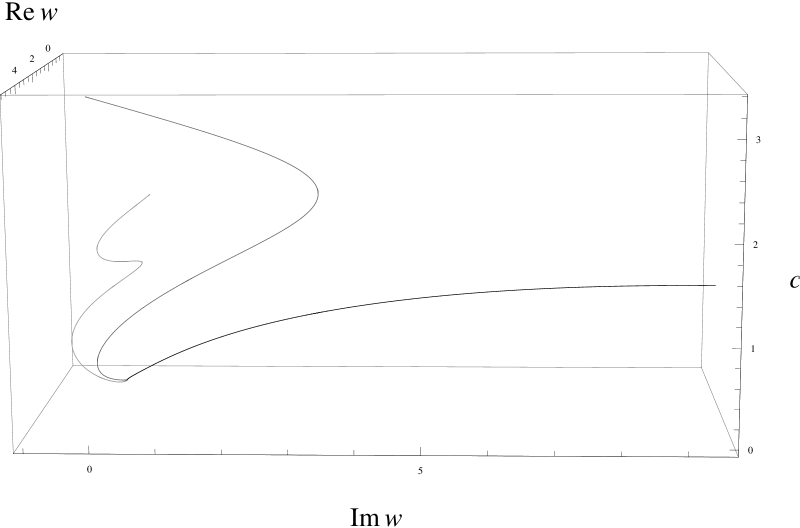
Figure 1. The above figure shows three geodesics in $\operatorname{\mathaccent 869{SU}}(1,1)$, all of length $\frac{3\pi}{2}$. The figure shows geodesics starting at $\tilde{1}$, which, when parametrized by arc length, have initial values of $\check{a}$ given (from left to right) by $-1,0$ and $\frac{3}{4}$.

4.2. Length and number of geodesics

Recall the definition of $\chi_{k}$ in (1). Then, up to reparameterization, we have the following results regarding the number of geodesics connecting $\tilde{1}$ and $\tilde{g}\in\operatorname{\mathaccent 869{SU}}(1,1)$.

Proposition 2.

• If $\tilde{g}=(c,0)$ for some $c$, then the number of geodesics is uncountable (countably many geometrically different).

• If $\tilde{g}=(0,w)$ for some $w$, then there exists a unique geodesic connecting $\tilde{g}$ and $\tilde{1}$. This geodesic is contained in the plane $c=0$.

• If $\tilde{g}$ is any other point, then we can obtain the number of geodesics in the following way. Let $k$ be the largest positive integer, such that

  $$|c|\geq\sqrt{|w|^{2}+\chi_{k}^{2}(1+|w|^{2})}-\chi_{k}-\tan^{-1}\left(\frac{\sqrt{|w|^{2}+\chi_{k}^{2}(1+|w|^{2})}-\chi_{k}}{1+\chi_{k}\sqrt{|w|^{2}+\chi_{k}^{2}(1+|w|^{2})}}\right).$$

  If there exists $k$, such that the above inequality is strict, then there are $2k+1$ geodesics connecting these two points. If $k$ gives the equality, then the number of geodesics is $2k$. If no such $k$ exists, then there is a unique geodesic.

Remark 4.

The number of geodesics in the case (c) above may be difficult to determine, but due to the fact that the value of $\sqrt{|w|^{2}+\chi_{k}^{2}+|w|^{2}\chi_{k}^{2}}-\chi_{k}-\tan^{-1}\left(\frac{\sqrt{|w|^{2}+\chi_{k}^{2}+|w|^{2}\chi_{k}^{2}}-\chi_{k}}{1+\chi_{k}\sqrt{|w|^{2}+\chi_{k}^{2}+|w|^{2}\chi_{k}^{2}}}\right)$, belongs to the interval $\Big{(}\pi k(\sqrt{|w|^{2}+1}-1),\,\,\pi(k+\frac{1}{2})(\sqrt{|w|^{2}+1}-1)\Big{)}$, this number remains between $2k_{1}-1$ and $2k_{1}+1$, where

$$k_{1}=\left\lceil\tfrac{|c|}{\pi(\sqrt{1+|w|^{2}}-1)}-\tfrac{1}{2}\right\rceil.$$

The proof is a long case by case analysis, and therefore, we leave it to section 6. Regarding to $\mathrm{(a)}$, we say that two geodesics are geometrically similar, if one is the image of another under an isometry. The isometry considered in $\mathrm{(a)}$ is $(c,w)\mapsto(c,e^{i\theta}w)$, $\theta\in\mathbb{R}$.

Since $\tilde{D}$ is a strongly bracket generating distribution (i.e. for every vector field $\tilde{X}_{0}$, $\tilde{D}$ and $[\tilde{X}_{0},\tilde{D}]$ span the entire tangent space at points where $X_{0}$ is nonvanishing), there are no abnormal length minimizers. Every geodesic may be extended indefinitely, therefore the Carnot-Carathéodory metric is complete (see [19] and [20]). Hence, every point is connected to $\tilde{1}$ by a length minimizing geodesic which is normal. The same holds for $\operatorname{SU}(1,1)$. The above information along with the proof of Proposition 2, leads to the following result.

Corollary 1.

• If $\tilde{g}\in e^{\operatorname{span}\{Z\}}$, then $d(\tilde{1};\tilde{g})=|c|$.

• If $\tilde{g}\in e^{\operatorname{span}\{X,Y\}}$, then $d(\tilde{1};\tilde{g})=\sinh^{-1}|w|$.

• If $\tilde{g}=(c,w)$ is neither in the vertical, nor in the horizontal space, and $|c|<|w|-\tan^{-1}|w|$, then

  $$d(\tilde{1};\tilde{g})=\tfrac{1}{\sqrt{1-\beta_{c,w}^{2}}}\sinh^{-1}\left(|w|\sqrt{1-\beta_{c,w}^{2}}\right),$$

  where $0<\beta_{c,w}<1$ is a unique number satisfying

  $$|c|=\tfrac{\beta_{c,w}}{\sqrt{1-\beta_{c,w}^{2}}}\sinh^{-1}\left(|w|\sqrt{1-\beta_{c,w}^{2}}\right)-\sin^{-1}\left(\tfrac{|w|\beta_{c,w}}{\sqrt{1+|w|^{2}}}\right).$$

• If $\tilde{g}=\left(\pm(|w|-\tan^{-1}|w|),w\right)$, then $d(\tilde{1};\tilde{g})=|w|.$

• If $\tilde{g}=(c,w)$ satisfies the inequality $|w|-\tan^{-1}|w|<|c|\leq\frac{\pi}{2}(\sqrt{|w|^{2}+1}-1)$, then

  $$d(\tilde{1};\tilde{g})=\tfrac{1}{\sqrt{\beta_{c,w}^{2}-1}}\sin^{-1}\left(|w|\sqrt{\beta_{c,w}^{2}-1}\right),$$

  where $1<\beta_{c,w}\leq\tfrac{\sqrt{1+|w|^{2}}}{|w|}$ is a unique number satisfying

  $$|c|=\tfrac{\beta_{c,w}}{\sqrt{\beta_{c,w}^{2}-1}}\sin^{-1}\left(|w|\sqrt{\beta_{c,w}^{2}-1}\right)-\sin^{-1}\left(\tfrac{|w|\beta_{c,w}}{\sqrt{1+|w|^{2}}}\right).$$

• If $\tilde{g}=(c,w)$ satisfies the inequality $\frac{\pi}{2}(\sqrt{|w|^{2}+1}-1)<|c|$, then

  $$d(\tilde{1};\tilde{g})=\tfrac{1}{\sqrt{\beta_{c,w}^{2}-1}}\left(\pi-\sin^{-1}\left(|w|\sqrt{\beta_{c,w}^{2}-1}\right)\right),$$

  where $1<\beta_{c,w}\leq\tfrac{\sqrt{1+|w|^{2}}}{|w|}$ is a unique number satisfying

  $$|c|=\tfrac{\beta_{c,w}}{\sqrt{\beta_{c,w}^{2}-1}}\left(\pi-\sin^{-1}\left(|w|\sqrt{\beta_{c,w}^{2}-1}\right)\right)-\left(\pi-\sin^{-1}\left(\tfrac{|w|\beta_{c,w}}{\sqrt{1+|w|^{2}}}\right)\right).$$

The details are again left to section 6. Notice that in all cases, the distance is independent of the sign of $c$, and of the argument of $w$.

Remark 5.

From these results for the universal cover, we easily obtain the following conclusions about the number of geodesics connecting 1 and $g\in\operatorname{SU}(1,1)$. It is

• uncountable (there are countably many geometrically different geodesics), if $g\in e^{\operatorname{span}\{Z\}}$.

• countable otherwise.

The next result we prove here.

Lemma 1.

Let $c_{1}$ and $c_{2}$ be two real numbers such that $|c_{1}|\leq|c_{2}|$. Then for any $w\in\operatorname{\mathbb{C}}$,

$$d(\tilde{1};(c_{1},w))\leq d(\tilde{1};(c_{2},w)).$$

Proof.

If $w=0$, then this follows from Corollary 1 (a). For $w\neq 0$, observe that the formulas for the distance in Corollary 1 (c) and (e) is increasing with respect to $\beta_{c,w}$, while the distance function in (f) is decreasing with respect to $\beta_{c,w}$. By taking upper and lower limits of the permitted values of $\beta_{c,w}$, we obtain that the cases (b) to (f) are given in the order of increasing distance.

To complete the proof, we need to show that in (c) and (e), $\beta_{c,w}$ is an increasing function with respect to $|c|$, while in (f), $\beta_{c,w}$ is a decreasing relative to $|c|$. We will only show that this holds in (e). The other cases are done similarly.

We need to differentiate

$$f(\beta)=\tfrac{\beta}{\sqrt{1-\beta^{2}}}\sinh^{-1}\left(|w|\sqrt{1-\beta^{2}}\right)-\sin^{-1}\left(\tfrac{|w|\beta}{\sqrt{1+|w|^{2}}}\right),$$

and see that the derivative is positive. This follows from the computation

$$\tfrac{\partial}{\partial\beta}f(\beta)=\tfrac{1}{1-\beta^{2}}\left(\tfrac{\sinh^{-1}(|w|\sqrt{1-\beta^{2}})}{\sqrt{1-\beta^{2}}}-\tfrac{|w|}{\sqrt{1+|w|^{2}(1-\beta^{2})}}\right)>0.$$

∎

Corollary 2.

If $g=(z_{1},z_{2})\in\operatorname{SU}(1,1)$, then $d(1;(z_{1},z_{2}))=d(\tilde{1};(\operatorname{Arg}\,z_{1},z_{2}))$.

Proof.

Since being a normal geodesic is a local property, it follows that any normal geodesic from 1 to $g$ in $\operatorname{SU}(1,1)$, has a unique lift to a curve starting at $\tilde{1}$, which is a normal geodesic of equal length to some point in $\pi^{-1}(g)$. This allows us to compute the length by the formula

$$d(1;g)=\min_{\tilde{g}\in\pi^{-1}(g)}\{d(\tilde{1};\tilde{g})\}.$$

To complete the proof of the Corollary, we need to show that for $g=(z_{1},z_{2})$, the point $(\operatorname{Arg}z_{1},z_{2})\in\pi^{-1}(g)$ has the minimal distance to $\tilde{1}$. Define $c_{0}=\operatorname{Arg}z_{0}$ and let $c_{k}=c_{0}+2\pi k$, $k\in\mathbb{Z}$. From the formula of the projection (6), any element in $\pi^{-1}(z_{1},z_{2})$ is of the form $(c_{k},z_{2})$. The rest follows from Lemma 1, since $|c_{0}|\leq|c_{k}|$. ∎

4.3. The cut and conjugate loci

For sub-Riemannian Lie groups satisfying Theorem 3, we define a sub-Riemannian analogue of the exponential map about the identity $1$ by

$$\exp_{sr}:\mathfrak{g}\setminus\mathfrak{k}\rightarrow G,\qquad X_{0}\mapsto e^{X}_{0}e^{-\operatorname{pr}_{\mathfrak{k}}X_{0}}.$$

For a more general definition of the exponential map in the sub-Riemannian setting, see [1]. We define the conjugate locus of $G$ from the identity 1, as the set of critical values of $\exp_{sr}$. We often split the conjugate locus in several sets, defining the $n$-th conjugate locus by the set $\{\exp tX_{0}\}$, where $X_{0}\in\mathfrak{g}\setminus\mathfrak{k}$, and t is so that there exist exactly $n$ values $0<t_{1}<\cdots<t_{n}=t$, so that $t_{j}X_{0}$ are all critical points. We define the cut locus from 1 as the set reachable by more than one minimizing geodesic.

Corollary 3.

The cut locus from $\tilde{1}$ for $\operatorname{\mathaccent 869{SU}}(1,1)$ is the vertical line. The cut locus from 1 for $\operatorname{SU}(1,1)$ consists of the points where $z_{1}<0$, as well as the points apart from the identity satisfying $z_{2}=0$.

Proof.

The cut locus for $\operatorname{\mathaccent 869{SU}}(1,1)$ follows from the proof of Proposition 2 and Corollary 1. For $\operatorname{SU}(1,1)$, if a point $(z_{1},z_{2})$ is in the cut locus, then either $c=\operatorname{Arg}\,z_{1},w=z_{2}$ is in the cut locus for $\operatorname{\mathaccent 869{SU}}(1,1)$ (which is the set of points $(c,0)$ for arbitrary $c\neq 0$) or there exist more than one $\tilde{g}\in\operatorname{\mathaccent 869{SU}}(1,1)$, such that $\pi(\tilde{g})=g$ and $d(\tilde{1};\tilde{g})=d(1;g)$. From the proof of Corollary 2, this only happens when $\operatorname{Arg}\,z_{1}=\pi$, in which there are two points of equal distance. ∎

The following proposition was proved for $\operatorname{SU}(1,1)$ in [4] (for the isometric case of $\operatorname{SL}(2)$), but here we generalize it, including the universal cover $\operatorname{\mathaccent 869{SU}}(1,1)$.

Proposition 3.

The $n$-th conjugate locus of $\tilde{1}\in\operatorname{\mathaccent 869{SU}}(1,1)$ consists of the vertical line, if $n$ is odd. If $n=2j$, then it consists of the points given by the equation

$$|c|=\sqrt{|w|^{2}+\chi_{j}^{2}+|w|^{2}\chi_{j}^{2}}-\chi_{j}-\tan^{-1}\left(\tfrac{\sqrt{|w|^{2}+\chi_{j}^{2}+|w|^{2}\chi_{j}^{2}}-\chi_{j}}{1+\chi_{j}\sqrt{|w|^{2}+\chi_{j}^{2}+|w|^{2}\chi_{j}^{2}}}\right).$$

Proof.

First, observe that from the definition of the exponential map (7) and Remark 2 in Section 3.1, $d\exp_{sr}$ exists only for $\check{a}\neq 0$. Put $w=u+iv$. Then we have

$$(c,u+iv)=\exp_{sr}\left(r\cos\theta X+r\sin\theta Y+a_{3}Z\right)$$

$$=\left(-\operatorname{\mathscr{T}}_{a}+a_{3},-r\operatorname{\mathscr{S}}_{r^{2}-a_{3}^{2}}\cos(\theta+a_{3})+ir\operatorname{\mathscr{S}}_{r^{2}-a_{3}^{2}}\sin(\theta+a_{3})\right).$$

The values of the elements of the matrix

$$\left(\begin{array}[]{ccccc}\frac{\partial}{\partial\theta}c&&\frac{\partial}{\partial\theta}u&&\frac{\partial}{\partial\theta}v\\ \frac{\partial}{\partial r}c&&\frac{\partial}{\partial r}u&&\frac{\partial}{\partial r}v\\ \frac{\partial}{\partial a_{3}}c&&\frac{\partial}{\partial a_{3}}u&&\frac{\partial}{\partial a_{3}}v\\ \end{array}\right),$$

become

$$\left(\begin{array}[]{ccccc}0&&rS\sin(\theta+a_{3})&&rS\cos(\theta+a_{3})\\ -\frac{a_{3}r}{r^{2}-a_{3}^{2}}\frac{1-CS}{C^{2}+a_{3}S^{2}}&&-\frac{(r^{2}C-a_{3}^{2}S)\cos(\theta+a_{3})}{r^{2}-a_{3}^{2}}&&\frac{(r^{2}C-a_{3}^{2}S)\sin(\theta+a_{3})}{r^{2}-a_{3}^{2}}\\ 1+\frac{a_{3}^{2}-r^{2}CS}{(r^{2}-a_{3}^{2})(C^{2}+a_{3}^{2}S^{2})}&&rS\sin(\theta)+\frac{ra_{3}(C-S)\cos(\theta+a_{3})}{r^{2}-a_{3}^{2}}&&rS\cos(\theta)-\frac{ra_{3}(C-S)\sin(\theta+a_{3})}{r^{2}-a_{3}^{2}}\\ \end{array}\right).$$

Here, we have simplified by writing just $S=\operatorname{\mathscr{S}}_{r^{2}-a_{3}^{2}}$ and $C=\operatorname{\mathscr{C}}_{r^{2}-a_{3}^{2}}$. The determinant of the above matrix is $\frac{r^{3}S(C-S)}{r^{2}-a_{3}^{2}}$. The value of $S$ vanishes at the points, for which $a_{3}^{2}-r^{2}=\pi^{2}k^{2},k\in\mathbb{N}$, and the image of such points is the vertical line (see the proof for Proposition 2 for more details). Moreover, $C-S$ vanishes only for $-\check{a}=\chi_{j}^{2}$. Hence, for a generic $X\in\mathfrak{g}\setminus\mathfrak{k}$, the point $tX$ can be singular for $\exp_{sr}$, only if $\check{a}<0$. Let us use the normalization $\check{a}=-\pi^{2}$. Let the $n$-th value $t_{n}$ be such that $t_{n}X$, is a singular point. Then it is clear that

$$t_{2j-1}=j,\qquad t_{2j}=\frac{\chi_{j}}{\pi},\qquad j\in\mathbb{N}.$$

Taking the image of these values under the map $\exp_{sr}$, we have the result. ∎

Remark 6.

Let $(c,w)\in\operatorname{\mathaccent 869{SU}}(1,1)$ be a point that does not belong to the vertical line (i.e. $w\neq 0$). Notice that if the value of $|c|$ from Proposition 2 increases (or the value of $|w|$ decreases), then (and only then) the number of geodesics increases when we pass through the even-indexed conjugate loci (see Figure 2).

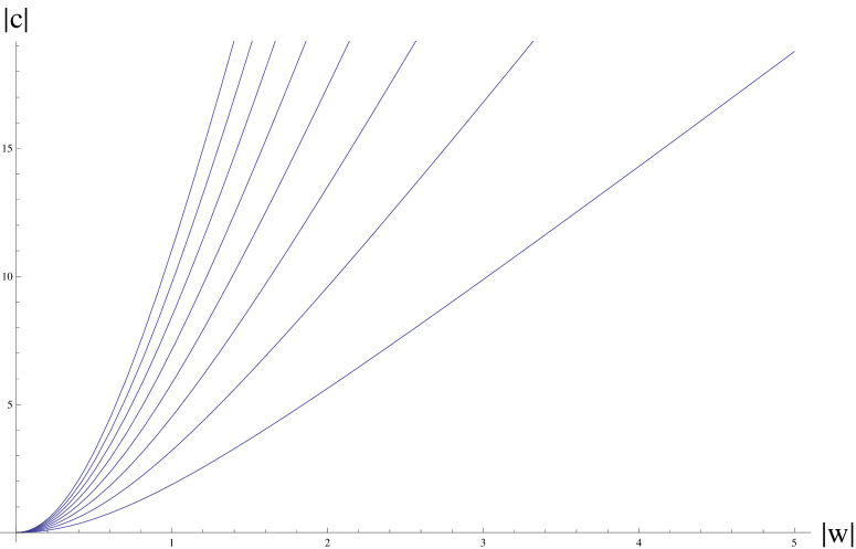
Figure 2. The above figure shows the eight first even conjugate loci. The horizontal axis corresponds to the values of $|w|$, and the values of $|c|$ occupy the vertical axis. Observe that a point under all the graphs is reachable by a unique geodesic. Then there are two geodesics in the 2-nd conjugate locus (that is the first graph). Between the 2-nd and the 4-th conjugate locus there are three, and so on.

Projecting the result in Corollary 3 by (6).

Corollary 4.

The $n$-th conjugate locus of $1\in\operatorname{SU}(1,1)$ for odd $n$ is the vertical line, and if $n=2j$, then it consists of the points

$$z_{1}=\frac{(-1)^{j}\left(1\mp i\sqrt{|z_{2}|^{2}(1+\chi_{j}^{2})+\chi_{j}^{2}}\right)e^{\pm i\sqrt{|z_{2}|^{2}(1+\chi_{j}^{2})+\chi_{j}^{2}}}}{\sqrt{1+\chi_{j}^{2}}}.$$

5. Sub-Lorentzian geometry on $\operatorname{\mathaccent 869{SU}}(1,1)$

5.1. Sub-Lorentzian maximizers and geodesics on $\operatorname{\mathaccent 869{SU}}(1,1)$

In contrast with the sub-Riemannian case, we only know that the relative maximizers exist locally. We have no guarantee of global existence of maximizers. Let us consider the distribution $\mathaccent 869{E}=\mathrm{span}\{\mathaccent 869{Y},\mathaccent 869{Z}\}$, with the metric $\tilde{\rho}$ restricted to $\mathaccent 869{E}$. We formulate an optimal control problem of maximizing

$$J(u,\tilde{g}_{u})=\int_{0}^{\tau}\sqrt{u_{1}^{2}-u_{2}^{2}}\,dt,\qquad u\in U=\left\{u\in\mathbb{R}^{2}|\,u_{1}=\sqrt{1+u_{2}^{2}}\right\},$$

where $\dot{\tilde{g}}_{u}=f(u,\tilde{g})=u_{1}\mathaccent 869{Z}(\tilde{g})+u_{2}\mathaccent 869{Y}(\tilde{g})$.

We only do the case when $\varkappa=1$. If $\varkappa=0$ one gets the same results, so it follows that there are no strictly abnormal geodesics. In order to use PMP, let us define the pseudo-Hamiltonian

$$\mathscr{H}(u,p_{1}X^{*}+p_{2}Y^{*}+p_{3}Z^{*})=\sqrt{u_{1}^{2}-u_{2}^{2}}+u_{1}p_{3}+u_{2}p_{2}$$

$$=1+p_{3}\sqrt{1+u_{2}^{2}}+p_{2}u_{2}.$$

where $u\in U=\{(u_{1},u_{2})\in\mathbb{R}^{2}|\,u_{1}=\sqrt{1+u_{2}^{2}}\}$. For the existence of $H(p)=\max_{u\in U}\mathscr{H}(p,u)$, we need that $|p_{3}|>|p_{2}|$ and that $p_{3}<0$. In this case

$$H(p_{1}X^{*}+p_{2}Y^{*}+p_{3}Z^{*})=1-\sqrt{p_{3}^{2}-p_{2}^{2}}.$$

This is from the fact that the optimal control is

$$u^{*}=\left(\tfrac{-p_{3}}{\sqrt{p_{3}^{2}-p_{2}^{2}}},\tfrac{p_{2}}{\sqrt{p_{3}^{2}-p_{2}^{2}}}\right).$$

Since $H$ cannot be extended to $T^{*}M\setminus s_{0}(M)$ (the tangent bundle with the zero-section removed), we solve the equation using the pseudo-Hamiltonian function $\mathscr{H}$ instead,

$$\dot{p}_{1}=\{p_{1},\mathscr{H}(u,\lambda)\}|_{u=u^{*}}=-2(u_{1}p_{2}+u_{2}p_{3})|_{u=u^{*}}=0,$$

$$\dot{p}_{2}=\{p_{2},\mathscr{H}(u,\lambda)\}|_{u=u^{*}}=2u_{1}p_{1}|_{u=u^{*}}=-\tfrac{2p_{1}p_{3}}{\sqrt{p_{3}^{2}-p_{2}^{2}}},$$

$$\dot{p}_{3}=\{p_{3},\mathscr{H}(u,\lambda)\}|_{u=u^{*}}=-2u_{2}p_{1}|_{u=u^{*}}=-\tfrac{2p_{1}p_{2}}{\sqrt{p_{3}^{2}-p_{2}^{2}}},$$

$p_{3}^{2}-p_{2}^{2}$ is a first integral in this case, and from the condition $\mathscr{H}(u,p_{1}X^{*}+p_{2}Y^{*}+p_{3}Z^{*})=0$, $p_{3}^{2}-p_{2}^{2}$ is equal to 1. We find the solutions (denote $p_{jo}:=p_{j}(0)$)

$$p_{1}(t)\equiv p_{1o},$$

$$p_{2}(t)=p_{2o}\cosh\left(2p_{1o}t\right)-p_{3o}\sinh\left(2p_{1o}t\right),$$

$$p_{3}(t)=p_{3o}\cosh\left(2p_{1o}t\right)-p_{2o}\sinh\left(2p_{1o}t\right).$$

Observe that $|p_{3o}|>|p_{2o}|$, and $p_{3o}<0$. Note also that $p_{3o}$ has to be equal to $-\sqrt{1+p_{2o}^{2}}.$ In order to simplify our calculation, we first solve it for $\operatorname{SU}(1,1)$, and then lift it to $\operatorname{\mathaccent 869{SU}}(1,1)$. We have to solve the following differential equation.

(8) $$\dot{g}=\left.\tfrac{\partial\mathscr{H}}{\partial p}\right|_{u=u^{*}}=-p_{3}Z(g)+p_{2}Y(g),$$

Make the following observation that

$$e^{a_{1}X}=\left(\begin{array}[]{cc}\cosh a_{1}&-\sinh a_{1}\\ -\sinh a_{1}&\cosh a_{1}\end{array}\right).$$

From this we notice that

$$e^{-a_{1}X}Z=Ze^{a_{1}X}=\cosh a_{1}Z+\sinh a_{1}Y,$$

$$e^{-a_{1}X}Y=Ye^{a_{1}X}=\cosh a_{1}Y+\sinh a_{1}Z,$$

$$e^{a_{1}X}X=Xe^{a_{1}X}=\cosh a_{1}X+\sinh a_{1}\cdot 1.$$

If we expand equation (8), we can write

$$\dot{g}=-\left(p_{3o}\cosh\left(2p_{1o}t\right)-p_{2o}\sinh\left(2p_{1o}t\right)\right)Z(g)+\left(p_{2o}\cosh\left(2p_{1o}t\right)-p_{3o}\sinh\left(2p_{1o}t\right)\right)Y(g)$$

$$=g(-p_{3o}Ze^{2tp_{1o}X}+p_{2o}Ye^{2tp_{1o}X})=ge^{-tp_{1}X}(-p_{3o}Z+p_{2o}Y)e^{tp_{1o}X},$$

and multiplying from the right by $e^{-ta_{1}X}$ and adding $-p_{1o}gXe^{-tp_{1o}X}=-p_{1o}ge^{-tp_{1o}X}X$ on both sides, we obtain

$$\dot{g}e^{-tp_{1o}X}-p_{1o}gXe^{-tp_{1o}X}=\tfrac{\partial}{\partial t}\left({g}e^{-tp_{1o}X}\right)=ge^{-tp_{1o}X}(-p_{3o}Z+p_{2o}Y-p_{1o}X).$$

It follows that

$$ge^{-tp_{1o}X}=e^{t(-p_{1o}X+p_{2o}Y-p_{3o}Z)},$$

i.e.,

$$g=e^{t(-p_{1o}X+p_{2o}Y-p_{3o}Z)}e^{tp_{1o}X}.$$

If we lift this curve and consider Theorem 3, then we easily get to the following proposition.

Proposition 4.

Assume that there exists a global length maximizing curve between $\tilde{1}$ and $\tilde{g}$. Then, this curve is a timelike, future-directed normal geodesic on the form

$$e^{t(a_{1}X+a_{2}Y+a_{3}Z)}e^{-ta_{1}X},$$

where $a_{3}>0$ and $|a_{2}|<a_{3}$.

Explicitly, by (7), these geodesics have the form

$$c(t)= - \operatorname{\mathscr{T}}_{ta}+\tan^{-1}\left(\tfrac{a_{2}\operatorname{\mathscr{C}}_{\check{a}}(t)\operatorname{\mathscr{S}}_{\check{a}}(t)-a_{1}a_{3}\operatorname{\mathscr{S}}_{\check{a}}(t)^{2}}{(1+|a_{1}+ia_{2}|^{2}|\operatorname{\mathscr{S}}_{\check{a}}(t)|^{2})\coth(a_{1}t)-a_{1}\operatorname{\mathscr{C}}_{\check{a}}(t)\operatorname{\mathscr{S}}_{\check{a}}(t)-a_{2}a_{3}\operatorname{\mathscr{S}}_{\check{a}}(t)^{2}}\right),$$

$$w(t)=(\operatorname{\mathscr{C}}_{\check{a}}(t)-ia_{3}\operatorname{\mathscr{S}}_{\check{a}}(t))\sinh(a_{1}t)-(a_{1}-ia_{2})\operatorname{\mathscr{S}}_{\check{a}}(t)\cosh(a_{1}t).$$

The projection of them to $\operatorname{SU}(1,1)$ is given by

$$z_{1}=(\operatorname{\mathscr{C}}_{\check{a}}(t)-ia_{3}\operatorname{\mathscr{S}}_{\check{a}}(t))\cosh(a_{1}t)-(a_{1}-ia_{2})\operatorname{\mathscr{S}}_{\check{a}}(t)\sinh(a_{1}t),$$

$$z_{2}=(\operatorname{\mathscr{C}}_{\check{a}}(t)-ia_{3}\operatorname{\mathscr{S}}_{\check{a}}(t))\sinh(a_{1}t)-(a_{1}-ia_{2})\operatorname{\mathscr{S}}_{\check{a}}(t)\cosh(a_{1}t).$$

We will discuss the situation when these curves correspond to length maximizers in Section 5.3.

5.2. Number of geodesics

The result in the sub-Lorentzian case is more complicated, than in the sub-Riemannian case. So we have to give some definitions in order to describe geodesics in a reasonable way. Write $\mathbb{N}_{0}$ for the collection of nonnegative integers. First, let us define a function $f_{\pm}:\mathbb{R}\times\mathbb{N}_{0}\rightarrow\mathbb{R}$, by

$$f_{\pm}(s;k)=\left\{\begin{array}[]{ll}\sqrt{1-s^{2}}&\text{if }|s|<1,\\ \mp\sinh\left(\frac{(2k\pm 1)\pi}{2}\sqrt{s^{2}-1}\right)&\text{if }|s|\geq 1.\end{array}\right.$$

Also, we define the numbers $\omega_{k},k\in\mathbb{N}$ as the numbers satisfying the equations

$$\frac{\omega_{k}}{\sqrt{1-\omega_{k}^{2}}}-\sin^{-1}\omega_{k}=\pi k,\qquad 0<\omega_{k}<1.$$

Finally, we define the function

$$F(s,\omega)=\sqrt{1-\omega^{2}}\cosh\sqrt{\frac{s^{2}-\omega^{2}}{1-\omega^{2}}}-\sqrt{s^{2}-\omega^{2}}\sinh\sqrt{\frac{s^{2}-\omega^{2}}{1-\omega^{2}}}.$$

Let us construct the following subsets of $\operatorname{\mathaccent 869{SU}}(1,1)$: $\Omega_{0}$ consists of all points

$$c=\operatorname{Arg}\left(x_{1}-i\sqrt{s^{2}+y_{2}^{2}}\right),\qquad w=\pm\sqrt{x_{1}^{2}+s^{2}-1}+iy_{2},$$

where $y_{2}\in\mathbb{R}$, $s>0$, and $x_{1}\in(-\infty,\,-\sqrt{1-s^{2}}]\bigcup[\sqrt{1-s^{2}},\,1-\frac{s^{2}}{2})$ when $s<1$, and $x_{1}\in(-\infty,\,1-\frac{s^{2}}{2})$ otherwise. Further, for $k\in\mathbb{N}$, define $\Omega_{k}$ as a set of all points

$$c=-\pi k+\operatorname{Arg}\left(x_{1}-i\sqrt{s^{2}+y_{2}^{2}}\right),\qquad w=\pm\sqrt{x_{1}^{2}+s^{2}-1}+iy_{2},$$

where $y_{2}\in\mathbb{R}$, $s>0$, and $x_{1}\in\mathbb{R}\setminus\left(-\sqrt{1-s^{2}},\sqrt{1-s^{2}}\right)$ for $s<1$, and $x_{1}\in(-\infty,F(s,\omega_{k})]$ otherwise. We split them into the following sets

• $A_{k}$ consist of all points

  $$c=-\pi k+\operatorname{Arg}\left(x_{1}-i\sqrt{s^{2}+y_{2}^{2}}\right),\qquad w=\pm\sqrt{x_{1}^{2}+s^{2}-1}+iy_{2},$$

  where $y_{2}\in\mathbb{R}$, $s>0$, and

  • $x_{1}\in\mathbb{R}\setminus\left(-\sqrt{1-s^{2}},\sqrt{1-s^{2}}\right)$, when $s\leq\omega_{k}$,

  • $x_{1}\in(-\infty,-\sqrt{1-s^{2}}]\cup(F(s,\omega_{k}),\infty)$, when $\omega_{k}<s<1$,

  • $x_{1}\in(-\infty,0]\cup\{F(1,\omega_{k})\}$, when $s=1$,

  • $x_{1}\in\{F(s,\omega_{k})\}$, when $s>1$.

• $B_{k}$ consist of all points

  $$c=-\pi k+\operatorname{Arg}\left(x_{1}-i\sqrt{s^{2}+y_{2}^{2}}\right),\qquad w=\pm\sqrt{x_{1}^{2}+s^{2}-1}+iy_{2},$$

  where $y_{2}\in\mathbb{R}$, $s>0$, and

  • $x_{1}\in\{\sqrt{1-s^{2}},F(s,\omega_{k})\}$, when $s<\omega_{k}$,

  • $x_{1}\in(0,F(s,\omega_{k}))$, when $s=1$,

  • $x_{1}\in(-\infty,F(s;k))$, when $s>1$.

• $C_{k}$ consist of all points

  $$c=-\pi k+\operatorname{Arg}\left(x_{1}-i\sqrt{s^{2}+y_{2}^{2}}\right),\qquad w=\pm\sqrt{x_{1}^{2}+s^{2}-1}+iy_{2},$$

  where $y_{2}\in\mathbb{R}$, $\omega_{k}<s<1$, and $x_{2}\in(\sqrt{1-s^{2}},F(s,\omega_{k}))$.

Let $\Xi_{k}=\{(-\pi k,x_{2})\in\operatorname{\mathaccent 869{SU}}(1,1)|\,x_{2}\in\mathbb{R}\}$. Finally, define

$$\Omega:=\Omega_{0}\,\cup\,\bigcup_{k=1}^{\infty}(\Omega_{k}\,\cup\,\Xi_{k}),\qquad\Xi:=\bigcup_{k=1}^{\infty}\Xi_{k},$$

$$A:=\Omega_{0}\,\cup\,\bigcup_{k=1}^{\infty}A_{k},\qquad B:=\bigcup_{k=1}^{\infty}B_{k},\qquad C:=\bigcup_{k=1}^{\infty}C_{k}.$$

Proposition 5.

There are timelike, future directed geodesics connecting $\tilde{1}$ and $\tilde{g}$, only if $\tilde{g}\in\Omega$. More precisely,

• the geodesic is unique if $\tilde{g}\in A$;

• there are two geodesics if $\tilde{g}\in B$;

• there are three geodesic if $\tilde{g}\in C$;

• there are countable many geodesics if $\tilde{g}\in\Xi$.

The proof for this is a case by case analysis, which we leave for section 6.3 .

Remark 7.

Let $\chi_{k}$ be the constants defined in (1) in Section 3.1. Then $\omega_{k}=|\sin\chi_{k}|$, so these numbers play a role here as well. However, unlike what was the case when we considered the sub-Riemannian geodesics, the mapping

$$a_{1}X+a_{2}Y+a_{3}Z\mapsto e^{a_{1}X+a_{2}Y+a_{3}Z}e^{-a_{1}X},$$

does not have any critical points satisfying $\check{a}=-\chi_{k}^{2}$.

We also remark the following interesting comparison with Lorentzian geometry.

Proposition 6.

The set reachable by Lorentzian geodesics starting at $\tilde{1}$, is the planes $\{(c,w)\in\operatorname{\mathaccent 869{SU}}(1,1)|\,c=-\pi k-\frac{\pi}{2},k\in\mathbb{N}\}$, along with all points satisfying $c<0$, $|w|<\tan|c|$, and $(c,w)=(-\pi k,0),k\in\mathbb{N}$. More precisely,

• there are uncountably many geodesics if $w=0$ (all geometrically similar, except for the case $c=0\text{ mod }\pi$, when they are uncountably many geometrically different).

• there is a unique geodesic if $w\neq 0$.

Proof.

A time-like geodesic $\tilde{g}(t)$, starting at $\tilde{1}$ satisfies $\tilde{g}(1)=e^{a_{1}X+a_{2}Y+a_{3}Z}$, and we know that $a_{3}>0$ and $a_{3}^{2}>a_{1}^{2}+a_{2}^{2}$ (and hence $\check{a}<0$). We rewrite the geodesics in terms of the parameters $k,\alpha^{\prime},r$ and $\theta$, where $\sqrt{-\check{a}}=\pi k+\alpha^{\prime},k\in\mathbb{N},\alpha^{\prime}\in(-\frac{\pi}{2},\frac{\pi}{2}]$ and $a_{1}+ia_{2}=re^{i\theta}$. The geodesics in these coordinates look like

$$c=-\tan^{-1}\left(\frac{\sqrt{r^{2}+(\pi k+\alpha^{\prime})^{2}}}{\pi k+\alpha^{\prime}}\tan\alpha^{\prime}\right)-k\pi,\qquad w=-\frac{r}{\pi k+\alpha^{\prime}}e^{i\theta}(-1)^{k}\sin\alpha^{\prime}.$$

Now $\theta$ can be determined by $\arg w$, and $k=\lceil-\frac{c}{\pi}-\frac{1}{2}\rceil$. Rewriting the equation for $|w|$ as

$$|w|^{2}+\sin^{2}\alpha^{\prime}=\frac{r^{2}+(\pi k+\alpha^{\prime})^{2}}{(\pi k+\alpha^{\prime})^{2}}\sin^{2}\alpha^{\prime},$$

and inserting it in the equation for $c$, we get that

$$\alpha^{\prime}=-\sin^{-1}\left(\tan(c)\sqrt{1-\frac{|w|^{2}}{\tan^{2}c}}\right),$$

for $c\neq\frac{\pi n}{2}$. For the remaining cases, $\alpha^{\prime}=0$ for $c=\pi n$, and $\alpha^{\prime}=\frac{\pi}{2}$ for $c=\frac{\pi}{2}+\pi n$. It is obvious that there are solutions only if $|\tan c|\geq|w|$. The equality can never be attained, because $\operatorname{sgn}\tan c=-\operatorname{sgn}\alpha^{\prime}$, which follows from

$$\tan c=-\frac{\sqrt{r^{2}+(\pi k+\alpha^{\prime})^{2}}}{\pi k+\alpha^{\prime}}\tan\alpha^{\prime}.$$

The equation

$$r^{2}=\frac{(\pi k+\alpha^{\prime})^{2}|w|}{\sin^{2}\alpha^{\prime}},$$

determines $r$ for $\alpha^{\prime}\neq 0$. When $\sin\alpha^{\prime}=0$, there are no restrictions on $r$. Also, if $|w|=0$, there are no restrictions on $\theta$. ∎

Proposition 6 yields that the set of points reachable by the Lorentzian geodesics starting at $\tilde{1}$ neither is contained, nor contains the set reachable from $\tilde{1}$ by the sub-Lorentzian geodesics. This contrasts the fact that the Lorentzian timelike future always contains the sub-Lorentzian one.

5.3. Lorentzian and sub-Lorentzian timelike future

Using the information we have collected, concerning sets reachable by geodesics, we obtain some results for the timelike future in general.

Figure 3. The above figure shows the lower bounds of Lorentzian and sub-Lorentzian timelike future for $\operatorname{\mathaccent 869{SU}}(1,1)$, showing the sub-Lorentzian future contained in the Lorentzian one. The negative direction of $c$ in the picture is upward. Remark that along the imaginary $w$-axis, $\mathcal{I}^{+}(\tilde{1},\tilde{\rho}|_{\tilde{E}})$ is tangent to $\mathcal{I}^{+}(\tilde{1},\rho)$.

Proposition 7.

• The timelike future of $\operatorname{\mathaccent 869{SU}}(1,1)$ with respect to the Lorentzian metric $\tilde{\rho}$, is given by

  $$\mathcal{I}^{+}(\tilde{1},\tilde{\rho})=\left\{(c,w)\in\operatorname{\mathaccent 869{SU}}(1,1)\,|\,c<-\tan^{-1}|w|\right\}.$$

• The timelike future of $\operatorname{\mathaccent 869{SU}}(1,1)$ with respect to the sub-Lorentzian metric $\tilde{\rho}|_{\tilde{E}}$, is given by

  $$\mathcal{I}^{+}(\tilde{1},\tilde{\rho}|_{\tilde{E}})=\{(c,w)\in\operatorname{\mathaccent 869{SU}}(1,1)\,|\,c<\operatorname{Arg}(1-|\operatorname{Re}w|-i\sqrt{(\operatorname{Im}w)^{2}+2|\operatorname{Re}w|})\}.$$

A picture of this is shown in Figure 3.

Proof.

Let us denote by $Q=\left\{(c,w)\in\operatorname{\mathaccent 869{SU}}(1,1)|\,c<-\tan^{-1}|w|\right\}$, and

$$\mathaccent 866{Q}=\{(c,w)\in\operatorname{\mathaccent 869{SU}}(1,1)|\,c<\operatorname{Arg}(1-|\operatorname{Re}w|-i\sqrt{(\operatorname{Im}w)^{2}+2|\operatorname{Re}w|})\}.$$

In both sub-Lorentzian and Lorentzian settings, information about the geodesics, imply that $Q$ and $\mathaccent 866{Q}$ are included in their respective timelike futures. To show the opposite inclusion, remark that in both Lorentzian and sub-Lorentzian settings, we use the fact that there exist relative length maximizers locally. So there exists a neighborhood $V$ of $\tilde{1}$, such that

$$\mathcal{I}^{+}(\tilde{1},\tilde{\rho}|_{V})=V\cap Q.$$

Define $U=V\cap Q$. Now from left invariance, we know that $\mathcal{I}^{+}(\tilde{g},\tilde{\rho})=L_{\tilde{g}}\mathcal{I}^{+}(\tilde{1},\tilde{\rho})$, and it follows that

$$\mathcal{I}^{+}(\tilde{1},\tilde{\rho})=\bigcup_{\tilde{g}\in\mathcal{I}^{+}(\tilde{1},\tilde{\rho})}L_{\tilde{g}}U.$$

Hence it is sufficient to show that $L_{\tilde{g}}U\subseteq Q$, for every $\tilde{g}\in Q$. Since every timelike curve from $\tilde{1}$ to a point outside $Q$ has to pass through the boundary $\partial Q$, it follows by continuity that it is sufficient to show that $L_{\tilde{g}_{0}}\overline{U}\subseteq L_{g_{0}}\overline{Q}\subseteq\overline{Q}$, for every $\tilde{g}_{0}\in\partial Q$. Here, $\overline{U}$ means the closure of $U$. Finally, since $L_{\tilde{g}_{0}}$ is an isomorphism, we have that $\partial L_{\tilde{g}_{0}}\overline{Q}=L_{\tilde{g}_{0}}\partial Q$, so all remaining arguments turn down to show that $\tilde{g}_{0}\tilde{g}\in\overline{Q}$ for every $\tilde{g}_{0},\tilde{g}\in\partial Q$. The same holds for $\mathaccent 866{Q}$.

In order to prove (a) we show that there are timelike geodesics connecting every point satisfying $-\frac{\pi}{2}\leq c<-\tan|w|$ with the origin. Let $(c,w)$ be an arbitrary point satisfying $c<-\frac{\pi}{2}$. Then we can construct a timelike curve from $\tilde{1}$, by taking a geodesic from $\tilde{1}$ to $(\frac{\pi}{2},iwe^{-ic})$, and then continue by a left translation of a geodesic from $\tilde{1}$ to $(c+\frac{\pi}{2},0)$.

Let $\tilde{g}_{0},\tilde{g}\in\partial Q$, $\tilde{g}_{0}=(-\tan^{-1}r_{0},r_{0}e^{i\theta_{0}}),\tilde{g}=(-\tan^{-1}r,re^{i\theta})$. First, if $r\geq 1$ and $r_{0}\geq 1$, then

$$\left(-\tan^{-1}r_{0},r_{0}e^{i\theta_{0}},-\tan^{-1}r,re^{i\theta}\right)=(C,W),$$

$$C=-\tan^{-1}r_{0}-\tan^{-1}r-\tan^{-1}\left(\frac{(rr_{0}-1)\sin\vartheta+(r+r_{0})\cos\theta}{\frac{1}{rr_{0}}+\frac{r}{r_{0}}+\frac{r_{0}}{r}+rr_{0}+(r+r_{0})\sin\vartheta-(rr_{0}-1)\cos\vartheta}\right),$$

$C\leq-\frac{\pi}{2},$ so in this case $(C,W)\in Q$. Here $\vartheta=\theta_{0}-\theta$.

We now turn to the case when either $r_{0}$ or $r$ is less than 1. If we denote

$$(x_{1}+iy_{1},z_{2}):=\pi(\tilde{g}_{0})\pi(\tilde{g}),$$

then we have

$$x_{1}=1-rr_{0}+rr_{0}\cos\vartheta,$$

$$y_{1}=-r_{0}-r+rr_{0}\sin\vartheta,$$

$$|z_{2}|^{2}=r^{2}+r_{0}^{2}+2r^{2}r_{0}^{2}+2rr_{0}\left((1-rr_{0})\cos\vartheta-(r+r_{0})\sin\vartheta\right)$$

$$=2(1-rr_{0})x_{1}+2(r+r_{0})|y_{1}|-(r+r_{0})^{2}-2(1-rr_{0}).$$

Since $r<1$ or $r_{0}<1$, we conclude that $y_{1}<0$. It follows that $\operatorname{Arg}(x_{1}+iy_{1})\leq-\tan^{-1}|z_{2}|=\operatorname{Arg}(1-i|z_{2}|)$, because $x_{1}\leq 1$. As a consequence, $g_{0}g\in\overline{Q}$.

Turning to (b), let us observe that $\Omega_{0}$ consist of all points, satisfying

$$-\pi+\tan^{-1}\left(\sqrt{\frac{(\operatorname{Im}w)^{2}}{1+(\operatorname{Re}w)^{2}}}\right)<c<\operatorname{Arg}(1-|\operatorname{Re}w|-i\sqrt{(\operatorname{Im}w)^{2}+2|\operatorname{Re}w|}).$$

Clearly all the points in $\Omega_{0}$ are in the timelike future. Pick up any point $(c,w)$ satisfying $c<\operatorname{Arg}(1-|\operatorname{Re}w|-i\sqrt{(\operatorname{Im}w)^{2}+2|\operatorname{Re}w|})$. Let $\gamma$ be a left translation by $(0,we^{-ic})$ of any geodesic connecting $\tilde{1}$ and $(c,0)$. The endpoint of $\gamma$ is $(c,w)$. Since $c<\operatorname{Arg}(1-|\operatorname{Re}w|-i\sqrt{(\operatorname{Im}w)^{2}+2|\operatorname{Re}w|})$, the curve $\gamma$ must at some point intersect $\Omega_{0}$. Pick up any point $\tilde{g}_{1}\in\gamma\cap\Omega_{0}$, travel from $\tilde{1}$ to $\tilde{g}_{1}$ along a geodesic, and continue along $\gamma$ to $(c,w)$.

Let $\tilde{g}_{0},\tilde{g}\in\mathaccent 866{Q}$ be of the form

$$g_{0}=\left(-\operatorname{Arg}(1-|x|-i\sqrt{y^{2}+2|x|}),x+iy\right),\,\,\,\tilde{g}=\left(-\operatorname{Arg}(1-|u|-i\sqrt{v^{2}+2|u|}),u+iv\right).$$

Assume first that $|u|\leq\frac{1}{2}$. If we again denote $\pi(\tilde{g}_{0})\pi(\tilde{g})=(x_{1}+iy_{1},x_{2}+iy_{2})$, we then obtain

$$x_{1}=(1-|x|)(1-|u|)+xu+vy-\sqrt{y^{2}+2|x|}\sqrt{v^{2}+2|u|},$$

$$x_{2}=(1-|x|)u+v\sqrt{y^{2}+2|x|}+x(1-|u|)-y\sqrt{v^{2}+2|u|}.$$

We only need to show that $1-x_{1}-|x_{2}|\geq 0$. Denote $\sigma=\operatorname{sgn}x_{2}$. Then

$$1-x_{1}-|x_{2}|=(|x|-\sigma x)+(|u|-\sigma u)-(|u|-\sigma u)(|x|-\sigma x)+(\sqrt{v^{2}+2|u|}-\sigma v)(\sqrt{y^{2}+2|x|}+\sigma y)$$

$$\geq(|x|-\sigma x)+(|u|-\sigma u)-(|u|-\sigma u)(|x|-\sigma x)\geq 0,$$

since $0\leq(|u|-\sigma u)\leq 1$. If $|u|>\frac{1}{2}$, the equality

$$\left(-1-|u|-i\sqrt{v^{2}+2|u|},u+iv\right)$$

$$=\left(1-\frac{i}{2}\frac{1}{\sqrt{v^{2}+2|u|}+\sigma_{1}v},-\frac{i}{2}\frac{\sigma_{1}}{\sqrt{v^{2}+2|u|}+\sigma_{1}v}\right)(1-|u_{1}|-i\sqrt{v_{1}^{2}+2|u_{1}|},u_{1}+iv_{1}),$$

where $\sigma_{1}=\operatorname{sgn}u$, and

$$u_{1}=u-\frac{\sigma_{1}}{2},\qquad v_{1}=\frac{\sigma_{1}}{2}\left(\sqrt{v^{2}+2|u|}+\sigma_{1}-\frac{2|u|-1}{\sqrt{v^{2}+2|u|}-\sigma_{1}v}\right),$$

tells us that $\tilde{g}$ may be written as a finite product of boundary elements, all with real part of the second coordinate of absolute value less than or equal to $\frac{1}{2}$. ∎

Since we know that locally, the Lorentzian or sub-Lorentzian causal future is the closure of the timelike future (see [13]), it follows from left invariance that $\mathcal{J}^{+}(\tilde{1},\tilde{\rho})$ and $\mathcal{J}^{+}(\tilde{1},\tilde{\rho}|_{\tilde{E}})$ are the closure of $\mathcal{I}^{+}(\tilde{1},\tilde{\rho})$ and $\mathcal{I}^{+}(\tilde{1},\tilde{\rho}|_{\tilde{E}})$, respectively.

Lemma 2.

Both with respect to the Lorentzian $\tilde{\rho}$ and the sub-Lorentzian metric $\tilde{\rho}|_{\tilde{E}}$, $\operatorname{\mathaccent 869{SU}}(1,1)$ is strongly causal.

Proof.

The proof is the same for both the Lorentzian and sub-Lorentzian cases. By left invariance, it is sufficient to find a strongly causal neighborhood. Let $U_{c_{0}},0<c_{0}<\frac{\pi}{2}$ be the set of all points $(c,w)$ in the timelike future of $\tilde{1}$ satisfying $c>-c_{0}$. Observe that inequality $|w|<\tan|c|$ must hold at the same time. Since, the causal future of all the elements in $U_{c_{0}}$ is contained in the causal future of $\tilde{1}$, any causal curve must exit through the surface $\{(-c_{0},w_{0})|\,|w_{0}|\leq\tan^{-1}c_{0}\}$. Then we need to show that for any such element $L_{(c_{0},w_{0})}U_{c_{0}}\cap U_{c_{0}}=\emptyset$. Observe that if $(c,w)\in U_{c_{0}}$ and $(-c_{0},w_{0})(c,w)=(C,W)$, then

$$C=-c_{0}+c+\operatorname{Arg}(\sqrt{(1+|w_{0}|^{2})(1+|w|^{2})}+w_{0}we^{-i(c+c_{0})})$$

$$\leq-c_{0}+c+\tan^{-1}\left(\frac{|w_{0}w|}{\sqrt{(1+|w_{0}|^{2})(1+|w|^{2})}}\right)<-c_{0}+c+\tan^{-1}(\sin c_{0}\sin|c|)$$

$$<-c_{0}+c+\tan^{-1}(\sin|c|)<c_{0}.$$

Hence, $U_{c_{0}}$ is strongly causal neighborhood of its elements. ∎

Proposition 8.

The distance between $\tilde{1}$ and $(c,w)$ with respect to the Lorentzian metric $\tilde{\rho}$ is equal to

$$d(\tilde{1};(c,w))=\left\{\begin{array}[]{ll}0&\text{if }c\geq-\tan^{-1}|w|\\ \sin^{-1}\left(\sqrt{\tan^{2}c-|w|^{2}}\right)&\text{if }-\frac{\pi}{2}<c<-\tan^{-1}|w|\\ \frac{\pi}{2}&\text{if }c=-\frac{\pi}{2}\\ \pi-\sin^{-1}\left(\sqrt{\tan^{2}c-|w|^{2}}\right)&\text{if }-\pi+\tan^{-1}<c<-\frac{\pi}{2}\end{array}\right.$$

When $c\leq-\pi+\tan^{-1}|w|$, we know that $d(\tilde{1};(c,w))\geq\pi$.

Proof.

The identity for $c\geq-\tan^{-1}|w|$ is trivial. For $-\pi+\tan^{-1}|w|<c<-\tan^{-1}|w|$, the formula follows from the fact that this space is globally hyperbolic, and from the proof of Proposition 6. The lower bound for the distance when $c\leq-\pi+\tan^{-1}|w|$ follows from the reverse triangle inequality, and from the fact that every such element has points in its timelike past of distance arbitrarily close to $\pi$.

To prove that $-\pi+\tan^{-1}|w|<c<-\tan^{-1}|w|$, we need to show that for every pair $\tilde{g}_{1},\tilde{g}_{2}$ in this subset, $\mathcal{J}^{+}(\tilde{g}_{1},\tilde{\rho})\cap\mathcal{J}^{-}(\tilde{g}_{2},\tilde{\rho})$ is compact. It is trivial that $\mathcal{J}^{+}(\tilde{g}_{1},\tilde{\rho})\subset\mathcal{J}^{+}(\tilde{1},\tilde{\rho})$, and by the same reasoning $\mathcal{J}^{-}(\tilde{g}_{2},\tilde{\rho})\subseteq\mathcal{J}^{-}((c_{0},0),\tilde{\rho})$. for some $-\pi<c_{0}<0$. Clearly,

$$\mathcal{J}^{-}((c_{0},0),\tilde{\rho})=\{(c,w)\in\operatorname{\mathaccent 869{SU}}(1,1)|\,c\geq c_{0}+\tan^{-1}|w|\}.$$

It follows that $\mathcal{J}^{+}(\tilde{1},\tilde{\rho})\cap\mathcal{J}^{-}((c_{0},0),\tilde{\rho})$, is compact for $-\pi<c_{0}<0$, but not when $c_{0}\leq-\pi$. ∎

One would expect an analogous statement for the sub-Lorentzian metric presenting a description of the distance function in $\Omega_{0}$, given the proof of Proposition 5, but it is more difficult to prove whether it is globally hyperbolic or not.

6. Proofs of main results

6.1. Proof of Proposition 2

6.1.1. Explanation of the proof and notation

The technique of this proof is to consider a general geodesic satisfying $\tilde{g}(0)=\tilde{1}$ and $\tilde{g}(1)=(c,w)$. Each geodesic is determined by their initial conditions $(a_{1},a_{2},a_{3})$, where $a_{1}^{2}+a_{2}^{2}\neq 0$. Our task will be, given the final point of the geodesic, $(c,w)$, to find how many choices of initial conditions do we have.

It will be practical to use $re^{i\theta}:=a_{1}+ia_{2}$. Notice that $\check{a}=r^{2}-a_{3}^{2}$, is independent of $\theta$. Whenever $r\neq 0$, we will use $\beta$ to denote the value $\beta:=\tfrac{a_{3}}{r}$. Notice that if $\beta\neq 0$, then $\check{a}=a_{3}^{2}(\beta^{-2}-1)$.

We need to solve the equations

(9) $$c=-\operatorname{\mathscr{T}}_{a}+a_{3},\qquad|w|=r|\operatorname{\mathscr{S}}_{r^{2}-a_{3}^{2}}|$$

(10) $$\frac{w}{|w|}=-e^{-i\theta}\frac{\operatorname{\mathscr{S}}_{r^{2}-a_{3}^{2}}}{|\operatorname{\mathscr{S}}_{r^{2}-a_{3}^{2}}|},\qquad\text{if }w\neq 0.$$

Recall the definition of $\operatorname{\mathscr{S}}_{\alpha},\check{a}$ and $\operatorname{\mathscr{T}}_{a}$ from Section 3.1.

We first deal with the special case $w=0$ right away. This implies $\operatorname{\mathscr{S}}_{r^{2}-a_{3}^{2}}=0$ (actually, it is an if and only if), so $\sqrt{a_{3}^{2}-r^{2}}=\pi k$, where $k\in\mathbb{N}$. Furthermore, $\operatorname{sgn}(c)=\operatorname{sgn}(a_{3})$, $|c|=|a_{3}|-\pi k$ and $r=\sqrt{a_{3}^{2}-\pi^{2}k^{2}}=\sqrt{c(c+2\pi k)}$, so there are countably many choices. Also, there are no restrictions to $\theta$.

For the rest of the proof, we will assume that $|w|\neq 0$ (and hence $-\check{a}\neq pi^{2}k^{2}$). Observe that this assumption means that given values of $r$ and $a_{3}$, (10) determines $e^{i\theta}$. We therefore only need to look at the number of solutions to (9). Since the expression for $\operatorname{\mathscr{T}}_{a}$ and $\operatorname{\mathscr{S}}_{\check{a}}$ vary with different choices of $a$, we need split the geodesics up into 4 different cases.

6.1.2. If $\beta=0$ (i.e. $a_{3}=0$)

The geodesics are contained in the horizontal space, and there is a unique one for every point ($r=\sinh^{-1}|w|$).

6.1.3. The case $\check{a}>0,\beta\neq 0\iff 0<|\beta|<1$.

In order to find a solution (9), we must solve the equations

(11) $$c=a_{3}-\tan^{-1}\left(\tfrac{\beta}{\sqrt{1-\beta^{2}}}\tanh\left(\tfrac{a_{3}\sqrt{1-\beta^{2}}}{\beta}\right)\right),$$

(12) $$\sinh\left(\tfrac{a_{3}\sqrt{1-\beta^{2}}}{\beta}\right)=|w|\sqrt{1-\beta^{2}}.$$

Observe that $c-\frac{\pi}{2}<a_{3}<c+\frac{\pi}{2}$. We rewrite (12) as

$$\tanh\left(\tfrac{a_{3}\sqrt{1-\beta^{2}}}{\beta}\right)=\sqrt{\tfrac{|w|^{2}(1-\beta^{2})}{1+|w|^{2}(1-\beta^{2})}},$$

and inserting it in (11), we obtain

$$a_{3}=c+\tan^{-1}\left(\tfrac{\beta|w|}{\sqrt{1+|w|^{2}(1-\beta^{2})}}\right).$$

Substituting $a_{3}$ back into (12), we have that $\beta$ is a solution to the equation $B(\beta)=0$, where $B$ is defined by

(13) $$B(\beta):=\tfrac{\sqrt{1-\beta^{2}}}{\beta}\left(c+\tan^{-1}\left(\tfrac{\beta|w|}{\sqrt{1+|w|^{2}(1-\beta^{2})}}\right)\right)-\sinh^{-1}(|w|\sqrt{1-\beta^{2}}).$$

This only vanishes when $0<|c|<|w|-\tan^{-1}|w|$, and this solution is unique.

To show this, we first make the observation that the limits

$$\lim_{|\beta|\rightarrow 1-}B(\beta)=0,\quad\lim_{|\beta|\rightarrow 0+}B(\beta)=\infty,$$

imply that a necessary condition for the existence of the solution to (13) is that the derivative $\frac{\partial}{\partial\beta}B$ vanishes at some point. Also, if the derivative vanishes exactly once on the interval $\beta\in(0,1)$, then this is a sufficient condition for $B$ to have at most one root on this interval. The same holds for the interval $\beta\in(-1,0)$. This derivative can be computed to be

(14) $$\tfrac{\partial}{\partial\beta}B(\beta)=-\tfrac{1}{\beta^{2}\sqrt{1-\beta^{2}}}\left(c+\tan^{-1}\left(\tfrac{|w|\beta}{\sqrt{1+|w|^{2}(1-\beta^{2})}}\right)-\tfrac{|w|\beta}{\sqrt{1+|w|^{2}(1-\beta^{2})}}\right).$$

Assume first that $c>0$. Then (14) has no zeros for $-1<\beta<0$. The derivative (14) vanishes at most once on the interval $0<\beta<1$. In fact, it vanishes exactly once only if $0<c<|w|-\tan^{-1}|w|$, while for greater values of $c$ it does not vanish. With this information together with the fact that for $0<c<|w|-\tan^{-1}|w|$ it holds that $\lim_{t\to 1-}\tfrac{\partial}{\partial\beta}B(\beta)<0$, we know that, in this case, (13) has one solution in $0<\beta<1$.

Similarly, it can be shown that (13) has exactly one solution, when $\tan^{-1}|w|-|w|<c<0$, and this solution $\beta$ is between -1 and 0. If $c=0$, (14) never vanishes in $\beta\in(-1,1)$.

6.1.4. The case $\check{a}=0\iff|\beta|=1$.

This happens when $r=|a_{3}|$. It is trivial that the equations

$$c=\tan^{-1}a_{3}+a_{3},\qquad|w|=|a_{3}|,$$

have a solution, which is unique, only if the endpoint satisfies the condition $c=\pm(|w|-\tan^{-1}|w|)$.

6.1.5. The case $\check{a}>0\iff|\beta|>1$:

For this part, we need the following lemma.

Lemma 3.

For $1\leq\beta\leq\sqrt{1+|w|^{-2}}$, define

$$\varphi_{1}:=\sin^{-1}\left(|w|\sqrt{\beta^{2}-1}\right),\qquad\varphi_{2}:=\sin^{-1}\left(\tfrac{|w|\beta}{\sqrt{1+|w|^{2}}}\right).$$

Then $(\beta+\sqrt{\beta^{2}-1})(\beta\varphi_{1}(\beta)-\sqrt{\beta^{2}-1}\varphi_{2}(\beta))$ monotonically increase from 0 to $\frac{\pi}{2}$ in the given interval.

Proof.

Let $1<\beta<\sqrt{1+|w|^{2}}.$ First, we observe that $\varphi_{1}$ and $\varphi_{2}$ have partial derivatives

$$\tfrac{\partial}{\partial\beta}\varphi_{1}(\beta)=\tfrac{\beta}{\sqrt{\beta^{2}-1}}\tfrac{|w|}{\sqrt{1-|w|^{2}(\beta^{2}-1)}},\qquad\tfrac{\partial}{\partial\beta}\varphi_{2}(\beta)=\tfrac{|w|}{\sqrt{1-|w|^{2}(\beta^{2}-1)}}.$$

Second, the identity

$$\sin^{-1}x<\sqrt{1+|w|^{2}}x\quad\text{ for values }\quad 0<x<\tfrac{|w|}{\sqrt{1+|w|^{2}}},$$

gives us an upper bound for $\varphi_{2}(\beta)-\varphi_{1}(\beta)$ by

$$\varphi_{2}(\beta)-\varphi_{1}(\beta) =\sin^{-1}\left(\tfrac{|w|(\beta-\sqrt{\beta^{2}-1})\sqrt{1-|w|^{2}(\beta^{2}-1)}}{\sqrt{1+|w|^{2}}}\right)$$

$$<|w|(\beta-\sqrt{\beta^{2}-1})\sqrt{1-(\beta^{2}-1)|w|^{2}}$$

We use this to make a lower bound for the derivative and complete the proof

$$\tfrac{\partial}{\partial\beta}\left((\beta+\sqrt{\beta^{2}-1})(\beta\varphi_{1}(\beta)-\sqrt{\beta^{2}-1}\varphi_{2}(\beta))\right)$$

$$= \tfrac{\beta+\sqrt{\beta^{2}-1}}{\sqrt{\beta^{2}-1}\sqrt{1-|w|^{2}(\beta^{2}-1)}}\left(|w|-\sqrt{1-|w|^{2}(\beta^{2}-1)}(\beta+\sqrt{\beta^{2}-1})(\varphi_{2}-\varphi_{1})\right)$$

$$> \tfrac{\beta+\sqrt{\beta^{2}-1}}{\sqrt{\beta^{2}-1}\sqrt{1-|w|^{2}(\beta^{2}-1)}}\Big{(}|w|-|w|\Big{(}1-(\beta^{2}-1)|w|^{2}\Big{)}\Big{)}$$

$$= \tfrac{|w|^{3}(\beta+\sqrt{\beta^{2}-1)}}{\sqrt{\beta^{2}-1}\sqrt{1-|w|^{2}(\beta^{2}-1)}}(\beta^{2}-1)>0.$$

∎

Equations (9) are now written in a more complicated form

(15) $$c=-\tan^{-1}\left(\tfrac{\beta}{\sqrt{\beta^{2}-1}}\tan\left(\tfrac{a_{3}\sqrt{\beta^{2}-1}}{\beta}\right)\right)-\pi\,\operatorname{sgn}(a_{3})\left\lceil\tfrac{\sqrt{-\check{a}}}{\pi}-\tfrac{1}{2}\right\rceil+a_{3},$$

(16) $$\left|\sin\left(\tfrac{a_{3}\sqrt{\beta^{2}-1}}{\beta}\right)\right|=|w|\sqrt{\beta^{2}-1}.$$

An immediate observation from (16), is that $|\beta|\leq\sqrt{1+|w|^{-2}}$. Let us introduce some notations. We write $\sqrt{-\check{a}}=\pi k+\alpha^{\prime},\alpha^{\prime}\in(-\tfrac{\pi}{2},\tfrac{\pi}{2}]\setminus\{0\}$, and also $\sigma_{1}=\operatorname{sgn}a_{3}=\operatorname{sgn}\beta$, $\sigma_{2}=\operatorname{sgn}\alpha^{\prime}$. If $k=0$, then $\sigma_{2}=1$. Subsequently,

$$\sin(\sqrt{-\check{a}})=(-1)^{k}\sigma_{2}|w|\sqrt{\beta^{2}-1},\qquad\cos(\sqrt{-\check{a}})=(-1)^{k}\sqrt{1-|w|^{2}(\beta^{2}-1)}.$$

So

$$a_{3}=c+\sigma_{2}\tan^{-1}\left(\tfrac{|w|\beta}{\sqrt{1-|w|^{2}(\beta^{2}-1)}}\right)+\sigma_{1}\pi k=c+\sigma_{2}\varphi_{2}(\beta)+\sigma_{1}\pi k,$$

$$\alpha^{\prime}=\sigma_{2}\tan^{-1}\left(\tfrac{|w|\sqrt{\beta^{2}-1}}{\sqrt{1-|w|^{2}(\beta^{2}-1)}}\right)=\sigma_{2}\varphi_{1}(\beta).$$

and it follows that $\beta$ has to be a solutions to the equation

(17) $$k\pi+\sigma_{2}(|\beta|+\sqrt{\beta^{2}-1})(|\beta|\varphi_{1}-\sqrt{\beta^{2}-1}|\varphi_{2}|)=|c|\sqrt{\beta^{2}-1}(|\beta|+\sqrt{\beta^{2}-1}),\vspace{0.3cm}$$

where

$$\beta\in\left[-\sqrt{1+|w|^{-2}},-1\right)\cup\left(1,\sqrt{1+|w|^{-2}}\right]\quad\text{ and }\quad\operatorname{sgn}\beta=\operatorname{sgn}c.$$

Also $\beta$ can only have the value $\pm\sqrt{1+|w|^{-2}}$, when $\sigma_{2}=1$. We need to count solutions for all values of $k$ and $\sigma_{2}=\pm 1$. See Figure 4 for a graphical representation of the equation (17).

From now we will just assume that $c>0$, since the considerations for $c<0$ are totally analogous. From Lemma 3, the left-hand side of (17) decreases or increases from $k\pi$ to $\frac{\pi}{2}(2k+\sigma_{2})$. This shows that there are no solutions for $k<0$. The derivative of the difference of the right and left side is given by

(18) $$\tfrac{\partial}{\partial\beta}\left(\left((c+\varphi_{2})\sqrt{\beta^{2}-1}-\beta\varphi_{1}\right)(\beta+\sqrt{\beta^{2}-1})\right)\\ =\tfrac{(\beta+\sqrt{\beta^{2}-1})^{2}}{\sqrt{\beta^{2}-1}}\left(c-\tfrac{|w|(\beta-\sqrt{\beta^{2}-1})}{\sqrt{1-|w|^{2}(\beta^{2}-1)}}+\varphi_{2}-\varphi_{1}\right),$$

and vanishes once if $c>|w|-\tan^{-1}|w|$, and otherwise it is negative. We therefore only need to check for roots for these values of $c$, in order find roots of (17).

If $k=0$, then there is only a solution when $\sigma_{2}=1$. In this case, there is a unique solution if $\tfrac{|w|-\tan^{-1}|w|}{\pi(\sqrt{|w|^{2}+1}-1)}\leq\tfrac{|c|}{\pi(\sqrt{|w|^{2}+1}-1)}\leq\tfrac{1}{2}$. The lower bound follows from (18), while the upper bound is from (17).

If $\sigma_{2}=-1$ and $k>0$, then there is a unique root if and only if, $k<\tfrac{|c|}{\pi(\sqrt{|w|^{2}+1}-1)}+\frac{1}{2}$. If $k>0$ and $\sigma_{2}=1$, then there is clearly no solutions for $k\geq\tfrac{|c|(\sqrt{|w|^{2}+1}+1)}{\pi|w|^{2}}$, and from (18), it follows that there is only one solution for $k<\frac{|c|}{\pi(\sqrt{|w|^{2}+1}-1)}-\frac{1}{2}$. For the cases between these, we define the number $\hat{\beta}$ as a root of the expression

$$c-\tfrac{|w|\left(\beta-\sqrt{\beta^{2}-1}\right)}{\sqrt{1-|w|^{2}(\beta^{2}-1)}}+(\varphi_{2}-\varphi_{1}),$$

i.e. point where the derivative in (18) vanishes. Then, there is a solution only if

$$k\pi+\left(\hat{\beta}+\sqrt{\hat{\beta}^{2}-1}\right)\left(\hat{\beta}\varphi_{1}-\sqrt{\hat{\beta}^{2}-1}\varphi_{2}\right)\leq c\sqrt{\hat{\beta}^{2}-1}\left(\hat{\beta}+\sqrt{\hat{\beta}^{2}-1}\right).$$

If the equality is attained in the above inequality, then $\chi_{k}=\tfrac{|w|\sqrt{\hat{\beta}^{2}-1}}{\sqrt{1+|w|^{2}-|w|^{2}\hat{\beta}^{2}}}$, i.e., $\hat{\beta}=\tfrac{\sqrt{1+|w|^{-2}+\chi_{k}^{-2}}}{\sqrt{1+\chi_{k}^{-2}}}$. Hence, there is only one solution when

$$|c|=\sqrt{|w|^{2}+\chi_{k}^{2}+|w|^{2}\chi_{k}^{2}}-\chi_{k}\tan^{-1}\left(\tfrac{\sqrt{|w|^{2}+\chi_{k}^{2}+|w|^{2}\chi_{k}^{2}}-\chi_{k}}{1+\chi_{k}\sqrt{|w|^{2}+\chi_{k}^{2}+|w|^{2}\chi_{k}^{2}}}\right),$$

and there are two solutions when $|c|$ is between this value and $\tfrac{\pi}{2}(2k+1)(\sqrt{|w|^{2}+1}-1)$. All the cases has now been examined, so this ends the proof.

Figure 4. This figure essentially summarizes the results of the proof of Proposition 2. The graph is based on the case $|w|=1$ and $|c|$ close to $\frac{5\pi}{2}(\sqrt{1+|w|^{-2}}-1)$, but the general idea is the for any point. The ”arches” in the graph are actually 7 different graphs, corresponding to different values of $\sigma_{2}$ and $k$ ($k$ is here from 0 to 3). The bottom half of the arches correspond to the case when $\sigma_{2}=1$, and the top for when $\sigma_{2}=-1$. The curve that is not an arch, is the right-hand side of (17). If $|c|$ is such that the graph of the right-hand side of (17) goes under all the above graphs, then the point corresponding to this choice of parameters is reached by a geodesic with $\check{a}\geq 0$, see Corollary 1 (c). If $|c|$ is less than $\frac{\pi}{2}(\sqrt{|w|^{-2}+1}-1)$, but not underneath the first arch, then this corresponds to the points in Corollary 1 (d). For larger values, the number of geodesics is equal to the number of intersections (so, in this case, for example, there are 5 geodesics). It is also easy to see that there can be only be either one root or no root when $\sigma_{2}=-\operatorname{sgn}(c)$, while if $\sigma_{2}=\operatorname{sgn}(c)$, the curve can either not intersect, be tangent (when $|c|$ is in the cut locus), or intersect twice, like the curve in our figure.

6.2. Proof of Corollary 1

Let us use the same notation as in the proof of Proposition 2. If $\tilde{g}(t)$ is a geodesic that goes from $\tilde{1}$ to $(c,w)$ in a unit time interval, then $\ell(\tilde{g})=r=\frac{a_{3}}{\beta}$. This implies (a)–(e) rather easily from the previous proof.

To prove (f), let $g_{k,\sigma_{2}}$ be a geodesic corresponding to a choice of $k$ and $\sigma_{2}$, with $\beta_{k,\sigma_{2}}$. The length becomes

$$\ell(\tilde{g}_{k,\sigma_{2}})=\frac{|c|+\sigma_{2}|\varphi_{2}|+k\pi}{\beta_{k,\sigma_{1}}}.$$

Then, from the equation $\sqrt{\beta_{k,\sigma_{2}}^{-2}-1}(|c|+\sigma_{2}|\varphi_{2}|+k\pi)=\pi k+\sigma_{2}\varphi_{1}$, we know that

$$\ell(g_{k,\sigma_{2}})^{2}=(|c|+k\pi+\sigma_{2}|\varphi_{2}(\beta_{k,\sigma_{2}})|)^{2}+(\pi k+\sigma_{2}\varphi_{1}(\beta_{k,\sigma_{2}}))^{2},$$

so

$$(|c|+k\pi)^{2}+(\pi k)^{2}<\ell(g_{k,1})^{2}\leq\left(|c|+\left(k+\frac{1}{2}\right)\pi\right)^{2}+\left(\pi\left(k+\frac{1}{2}\right)\right)^{2},$$

$$\left(|c|+(k-\frac{1}{2})\pi\right)^{2}+\left(\pi(k-\frac{1}{2})\right)^{2}\leq\ell(g_{k,-1})^{2}<(|c|+k\pi)^{2}+(\pi k)^{2}.$$

It follows that $\tilde{g}_{1,-1}$ is minimal.

6.3. Proof of Proposition 5

6.3.1. Explanation of the proof and notation

Since we are working with timelike-future directed curves, we know that $a_{3}>0$ and that $|a_{2}|<a_{3}$. Let us therefore denote $a_{3}=r\cosh\theta$, and $a_{2}=r\sinh\theta$. Then $\check{a}=a_{1}^{2}-r^{2}$. Similarly to the sub-Riemannian geodesics, we consider $\tilde{g}(0)=\tilde{1},$ $\tilde{g}(1)=(c,w)$, and look at how the final point defines the initial conditions. We are going to use the projection of $(c,w)$ to $\operatorname{SU}(1,1)$. Along with the coordinates $z_{1}=x_{1}+iy_{1}$ and $z_{2}=x_{1}+iy_{2}$, we shall use new coordinates given by

$$u_{1}=x_{1}+x_{2},\quad u_{2}=x_{1}-x_{2},\quad v_{1}=y_{1}+y_{2},\quad v_{2}=y_{1}-y_{2}.$$

Observe that $|z_{1}|^{2}-|z_{2}|^{2}=u_{1}u_{2}+v_{1}v_{2}=1$. Recall the definition of $\check{a},\operatorname{\mathscr{C}}_{\check{a}},\operatorname{\mathscr{S}}_{\check{a}}$ and $\operatorname{\mathscr{T}}_{a}$ from Section 3.1.

The projection of the geodesics to these coordinates becomes

$$\begin{array}[]{ll}u_{1}=e^{a_{1}}\left(\operatorname{\mathscr{C}}_{\check{a}}-a_{1}\operatorname{\mathscr{S}}_{\check{a}}\right),&u_{2}=e^{-a_{1}}\left(\operatorname{\mathscr{C}}_{\check{a}}+a_{1}\operatorname{\mathscr{S}}_{\check{a}}\right),\\ v_{1}=-r\operatorname{\mathscr{S}}_{\check{a}}e^{a_{1}-\theta},&v_{2}=-r\operatorname{\mathscr{S}}_{\check{a}}e^{-(a_{1}-\theta)}.\end{array}$$

The relationship between the projected coordinates and the original ones on the covering space is

$$c=-\operatorname{\mathscr{T}}_{a}+\tan^{-1}\left(\frac{2\sinh a_{1}(u_{2}v_{1}-u_{1}v_{2})}{e^{-a_{1}}(u_{1}^{2}+v_{1}^{2}+1)+e^{a_{1}}(u_{2}^{2}+v_{2}^{2}+1)}\right),$$

$$w=\tfrac{1}{2}(u_{1}-u_{2}+i(v_{1}-v_{2})).$$

Furthermore,

(19) $$2\operatorname{\mathscr{C}}_{a_{1}^{2}-r^{2}}=u_{1}e^{-a_{1}}+u_{2}e^{a_{1}},$$

(20) $$2a_{1}\operatorname{\mathscr{S}}_{a_{1}^{2}-r^{2}}=-u_{1}e^{-a_{1}}+u_{2}e^{a_{1}},$$

(21) $$2r\sinh(\theta)\operatorname{\mathscr{S}}_{a_{1}^{2}-r^{2}}=v_{1}e^{-a_{1}}-v_{2}e^{a_{1}},$$

(22) $$2r\cosh(\theta)\operatorname{\mathscr{S}}_{a_{1}^{2}-r^{2}}=-v_{1}e^{-a_{1}}-v_{2}e^{a_{1}}.$$

We will use this coordinates to compute the number of geodesics. We are again forced to split into different cases.

Some of these cases we need to deal with right away. First, let us consider the case when $a_{1}^{2}-r^{2}=-\pi^{2}k^{2},k\in\mathbb{N}$. The only points that can be reached by this type of geodesics are $(-\pi k,x_{2})$. Then

$$a_{1}=(-1)^{k}\sinh^{-1}x_{2},\qquad r=\sqrt{c^{2}+(\sinh^{-1}x_{2})^{2}},$$

and there are no restrictions on $\theta$.

Otherwise, if $a_{1}^{2}-r^{2}\neq-\pi^{2}k^{2}$, then $v_{1}v_{2}=1-u_{1}u_{1}>0$. It follow that

(23) $$\theta=a_{1}+\log\sqrt{\tfrac{v_{2}}{v_{1}}},\quad\text{and}\quad r=\tfrac{2\sqrt{v_{1}v_{2}}|a_{1}|}{|u_{2}e^{a_{1}}-u_{1}e^{-a_{1}}|}\quad\text{if }a_{1}\neq 0.$$

Hence, when $a_{1}\neq 0$, we only need to find the number of solutions to the equation (20) with respect to $a_{1}$. From this, the values of $r$ and $\theta$ will be determined by (23). Remark that (23) also give us the expression

(24) $$\check{a}=\left(\frac{a_{1}}{\frac{u_{2}}{2}e^{a_{1}}-\frac{u_{1}}{2}e^{-a_{1}}}\right)^{2}\left(\left(\tfrac{u_{2}}{2}e^{a_{1}}+\tfrac{u_{1}}{2}e^{-a_{1}}\right)^{2}-1\right),\quad a_{1}\neq 0.$$

6.3.2. If $a_{1}=0$:

We find $r$ as $r=k+(-1)^{k+1}\sin^{-1}\left(\tfrac{(v_{1}+v_{2})\sqrt{v_{1}v_{2}}}{|v_{1}|+|v_{2}|}\right)$, where $k=\lceil\frac{c}{\pi}-\frac{1}{2}\rceil$. There will now be exactly one geodesic, satisfying $a_{1}=0$, when $(c,w)$ is of the form

$$c=-\pi k+\operatorname{Arg}(\sqrt{1-s^{2}}-\operatorname{sgn}(s)i\sqrt{y_{2}^{2}+s^{2}}),\quad w=iy_{2},$$

where $y_{2}\in\mathbb{R},s\in(-1,1]\setminus\{0\}$ or $s\in(0,1]$ if $k=0$.

6.3.3. If $\check{a}>0$:

A quick look at (21) and (22) yields that $v_{1}<0$ and $v_{2}<0$. Also from (19), we know that at least one of $u_{1}$ and $u_{2}$ is positive. We define $b=\sqrt{\left(\frac{u_{2}}{2}e^{a_{1}}+\frac{u_{1}}{2}e^{-a_{1}}\right)^{2}-1}$. Then

$$e^{a_{1}}=\tfrac{\sqrt{b^{2}+1}+\sigma_{1}\sqrt{b^{2}+s^{2}}}{u_{2}}=\tfrac{u_{1}}{\sqrt{b^{2}+1}-\sigma_{1}\sqrt{b^{2}+s^{2}}},\quad\sigma_{1}=\pm 1.$$

Here, we denote $s=\sigma_{1}\sqrt{v_{1}v_{2}}.$ Notice, that the first part of the above equation is not valid if $u_{2}=0$, and the second part is not valid if $u_{1}=0$. The relation (20) implies $\operatorname{sgn}a_{1}=\sigma_{1}$.

If $\sigma_{1}=1$, then we know that $\operatorname{sgn}u_{2}=1$. Furthermore, from (20), we obtain that $b$ is a solution to the equation

(25) $$\psi_{-1}(b)-u_{2}=0,\qquad\mbox{where \ }\psi_{-1}(b):=(\sqrt{b^{2}+1}+\sqrt{b^{2}+s^{2}})e^{-\frac{\sqrt{b^{2}+s^{2}}}{b}\log(b+\sqrt{b^{2}+1})},$$

$\psi_{-1}$ increases from $(1+s)e^{-s}$ to 1, so a solution exists only if $(1+s)e^{-s}<u_{2}<1$. Then the points, which are connected by these types of geodesics are

$$c=\operatorname{Arg}\left(\frac{u_{2}^{2}+1-s^{2}}{2u_{2}}-i\sqrt{y_{2}^{2}+s^{2}}\right),\qquad w=\frac{1-s^{2}-u_{2}^{2}}{2u_{2}}+iy_{2},$$

where $(1+s)e^{-s}<u_{2}<1$. To get some idea of the meaning the above equations, notice that $\operatorname{sgn}(1-s)=\operatorname{sgn}u_{1}$, so $x_{1}=\frac{1}{2}(\frac{1-s^{2}}{u_{2}}+u_{2})$ is an increasing function of $u_{2}$ when $s>1$. Also, $x_{2}=\frac{1}{2}(\frac{1-s^{2}}{u_{2}}-u_{2})$ is a decreasing function of $u_{2}$ when $s<1$. Using this information, we know that there are only geodesic of these types connecting the points of the form

$$c=\operatorname{Arg}\left(x_{1}-i\sqrt{s^{2}+y_{2}^{2}}\right),\qquad w=x_{2}+iy_{2},$$

with the identity of the group, where $y_{2}\in\mathbb{R},s>0$ and $x_{1},x_{2}$ satisfy one of the following conditions

• $x_{2}\in(-\frac{s^{2}}{2},\sinh s-s\cosh s)$, $x_{1}=\sqrt{x_{2}^{2}+1-s^{2}}$, if $0<s<1$;

• $x_{1}=-x_{2}\in(e^{-1},\frac{1}{2})$, if $s=1$;

• $x_{1}\in(\cosh s-s\sinh s,1-\frac{s^{2}}{2}),x_{2}=-\sqrt{x_{1}^{2}+s^{2}-1}$, if $s>1$.

We can rewrite the above cases as the condition $x_{2}=-\sqrt{x_{1}^{2}+1-s^{2}}$, $x_{1}\in(\cosh s-s\sinh s,1-\frac{s^{2}}{2})$.

When $\sigma_{1}=-1$, we know that $\operatorname{sgn}u_{1}=1$, and $b$ is a solution to the equation $\psi_{-1}(b)=\log u_{1}$. So the points reachable by these types of geodesics are

$$c=\operatorname{Arg}\left(x_{1}-i\sqrt{y_{2}^{2}+s^{2}}\right),\qquad w=x_{2}+iy_{2},$$

where $s<0,y_{2}\in\mathbb{R}$, and $x_{1},x_{2}$ satisfy one of the following conditions

• $x_{2}\in(\sinh s-s\cosh s,\frac{s^{2}}{2}),x_{1}=\sqrt{x_{2}^{2}+1-s^{2}}$, if $0>s>-1$;

• $x_{1}=x_{2}\in(e^{-1},\frac{1}{2})$ if $s=-1$;

• $x_{1}\in(\cosh s-s\sinh s,1-\frac{s^{2}}{2}),x_{2}=\sqrt{x_{1}^{2}+s^{2}-1}$, if $s<-1$.

Notice that the only thing that changes with the sign of $\sigma_{1}$, is the sign of $x_{2}$.

6.3.4. If $\check{a}=0$:

From (19) and (20), it follows that there are geodesics only of this type connecting the initial point with every point of the form

$$\left\{\left.\left(\operatorname{Arg}\left(\cosh s-s\sinh s-i\sqrt{s^{2}+y_{2}^{2}}\right),\sinh s-s\cosh s+iy_{2}\right)\right|s,y_{2}\in\mathbb{R},s\neq 0\right\}.$$

6.3.5. If $\check{a}<0$:

We introduce the notation $\sqrt{-\check{a}}=\pi k+\alpha^{\prime},\alpha^{\prime}\in\left(-\tfrac{\pi}{2},\tfrac{\pi}{2}\right]\setminus\{0\}$. Let $\sigma_{2}=\operatorname{sgn}\alpha^{\prime}$. Notice that $\operatorname{sgn}v_{1}=\operatorname{sgn}v_{2}=(-1)^{k+1}\sigma_{2}$, and hence, $\operatorname{sgn}y_{1}=(-1)^{k+1}\sigma_{2}$. Now define

$$\varphi_{1}:=\tan^{-1}\left(\tfrac{r\cosh\theta}{\sqrt{-\alpha}}\tan\alpha^{\prime}\right),\qquad\varphi_{2}:=\tan^{-1}\left(\tfrac{2(u_{2}v_{1}-u_{1}v_{2})\sinh a_{1}}{e^{-a_{1}}(u_{1}^{2}+v_{1}^{2}+1)+e^{a_{1}}(u_{2}^{2}+v_{2}^{2}+1)}\right),$$

so that $c=-\pi k-\varphi_{1}+\varphi_{2}$. From the fact that $\sin c=(-1)^{k+1}\sin(\varphi_{1}-\varphi_{2})=y_{1}$, we know that $\operatorname{sgn}(\varphi_{1}-\varphi_{2})=\operatorname{sgn}\varphi_{1}=\sigma_{2}$, which yields that $k=-\lceil\tfrac{c}{\pi}\rceil-\tfrac{1-\sigma_{2}}{2}.$ Now write $c=2n\pi+\operatorname{Arg}(z_{1})$. Then, $2n=k+\tfrac{(1+(-1)^{k+1})\sigma_{2}}{2}$, so

$$c=\left\{\begin{array}[]{ll}-\pi k+\operatorname{Arg}(-z_{1}),&\text{if {\it k} is odd;}\\ -k\pi+\operatorname{Arg}(z_{1}),&\text{if {\it k} is even.}\end{array}\right.$$

Given a value of $k$, the value of $c$ is completely defined by $z_{1}$. We also know that if two geodesics has the same endpoint, then the maximal difference in their value of $k$ is 1.

We need to find $a_{1}$ as a solution to

$$\frac{2a_{1}\sqrt{1-\left(\frac{u_{2}}{2}e^{a_{1}}+\frac{u_{1}}{2}e^{-a_{1}}\right)^{2}}}{u_{2}e^{a_{1}}-u_{1}e^{-a_{1}}}=\sigma_{2}(-1)^{k}\pi k+(-1)^{k}\sin^{-1}\left(\sqrt{1-\left(\tfrac{u_{2}}{2}e^{a_{1}}+\tfrac{u_{1}}{2}e^{-a_{1}}\right)^{2}}\right).$$

Let us denote $b=\sqrt{1-\left(\frac{u_{2}}{2}e^{a_{1}}+\frac{u_{1}}{2}e^{-a_{1}}\right)^{2}}$. It follows that

$$e^{a_{1}}=\tfrac{(-1)^{k}(\sqrt{1-b^{2}}+\sigma_{1}\sqrt{v_{1}v_{2}-b^{2}})}{u_{2}}=\tfrac{u_{1}}{(-1)^{k}(\sqrt{1-b^{2}}-\sigma_{1}\sqrt{v_{1}v_{2}-b^{2}})},\quad\sigma_{1}=\pm 1.$$

As in the previous cases, there are some obvious restrictions on the values of $u_{2}=0$ or $u_{1}=0$. Here we used that $\operatorname{sgn}\left(\tfrac{u_{2}}{2}e^{a_{1}}+\tfrac{u_{1}}{2}e^{-a_{1}}\right)=(-1)^{k},$ because of (19). From (20), we know that $\sigma_{1}=\sigma_{2}\,\operatorname{sgn}a_{1}$.

If $\sigma_{1}=1$, then $\operatorname{sgn}u_{2}=(-1)^{k}$, and so $b$ is a solution to

$$\psi_{k}(b)=(-1)^{k}u_{2},\quad\psi_{k}(b):=\left(\sqrt{1-b^{2}}+\sqrt{s^{2}-b^{2}}\right)e^{-\frac{\sqrt{s^{2}-b^{2}}}{b}(\sigma_{2}\pi k+\sin^{-1}b)},$$

where $0<b\leq\min\{1,|s|\}$. Again we use the notation $s=\sigma_{1}\sqrt{v_{1}v_{2}}$. The upper bound for $b$ is strict, unless $|q_{1}|>1$ and $\sigma_{2}=1$, because $\alpha^{\prime}$ can be $\frac{\pi}{2}$, but not $-\frac{\pi}{2}$. Moreover, from (20), $b=|s|$ implies that either $a_{1}=0$ or $\sin\sqrt{-\check{a}}=0$, the case which already excluded. Similarly, when $\sigma_{1}=-1$, so $b$ is a solution to $\psi_{k}(b)=(-1)^{k}u_{1}$.

We investigate when a solution can exist.

• We start with the special case $k=0$. Then $\psi_{0}$ decreases from $(1+|s|)e^{-|s|}$ to $\sqrt{s^{2}-1}e^{-\frac{\pi}{2}\sqrt{s^{2}-1}}$ for $s\geq 1$, and from $(1+|s|)e^{-|s|}$ to $\sqrt{1-s^{2}}$ for $|s|<1$.

• If $\sigma_{2}=-1$, then $\psi_{k}$ decreases from $\infty$ to $\sqrt{1-s^{2}}$ for $|s|<1$, or to

  $$\sqrt{s^{2}-1}\exp\left(\tfrac{(2k-1)\pi}{2}\sqrt{s^{2}-1}\right)$$

  otherwise.

• If $\sigma_{2}=1$, then $\psi_{k}$ increases from $0$ to $\sqrt{1-s^{2}}$ for $|s|\leq\omega_{k}$. Continuing with $\sigma_{2}=1$, if $|s|>\omega_{k}$, then $\psi_{k}$ increases from $0$ to $(\sqrt{1-\omega_{k}^{2}}+\sqrt{s^{2}-\omega_{k}^{2}})\exp\left(-\sqrt{\frac{s^{2}-\omega_{k}^{2}}{1-\omega_{k}^{2}}}\right)$, and decreases to $\sqrt{1-s^{2}}$ for $|s|<1$, or to $\sqrt{s^{2}-1}\exp\left(-\frac{(2k+1)\pi}{2}\sqrt{s^{2}-1}\right)$ otherwise.

Further, if $\sigma_{1}=1$, then $\operatorname{sgn}u_{2}=(-1)^{k}$, and $\operatorname{sgn}u_{1}=(-1)^{k}\operatorname{sgn}(1-s^{2})$, and the same holds when $\sigma_{1}=-1$, interchanging $u_{1}$ and $u_{2}$. Also, from

$$x_{1}=\frac{1}{2}\left(u_{1}+\frac{1-s^{2}}{u_{1}}\right)=\frac{1}{2}\left(\frac{1-s^{2}}{u_{2}}+u_{2}\right),\quad x_{2}=\frac{1}{2}\left(u_{1}-\frac{1-s^{2}}{u_{1}}\right)=\frac{1}{2}\left(\frac{1-s^{2}}{u_{2}}-u_{2}\right),$$

we know that $x_{1}$ is an increasing function of $u_{1}$ and $u_{2}$, when $|s|>1$. When $|s|<1$, $x_{2}$ increases in $u_{1}$ and decreases in $u_{2}$. As a result, we know which point is reachable by which type of geodesics. We only show the results for $s>0$, since for $s<0$, the results are the same, only with different sign for $x_{2}$.

• If $k=0$, then

  • if $0<s<1$, then $x_{1}=\sqrt{x_{2}^{2}+1-s^{2}}$, $x_{2}\in(\sinh s-s\cosh s,0)$;

  • if $1\leq s$, $x_{2}=-\sqrt{x_{1}^{2}+s^{2}-1}$, $x_{1}\in[f_{+}(s;0),\cosh s-s\sinh s)$.

• If $k>0$ and $\sigma_{2}=-1$, then

  • if $0<s<1$, $(-1)^{k}x_{1}=\sqrt{x_{2}^{2}+1-s^{2}}$, and $(-1)^{k}x_{2}\in(-\infty,0)$;

  • if $s\geq 1$, $(-1)^{k}x_{2}=-\sqrt{x_{1}^{2}+s^{2}-1}$, and $(-1)^{k}x_{1}\in(f_{-}(s;k),\infty)$.

• If $k>0$ and $\sigma_{2}=1$, then there is one geodesic (list 1)

  • if $0<s\leq\omega_{k}$, $(-1)^{k}x_{1}=\sqrt{x_{2}^{2}+1-s^{2}}$, and $(-1)^{k}x_{2}\in(0,\infty)$;

  • if $\omega_{k}<s<1$, $(-1)^{k}x_{1}=\sqrt{x_{2}^{2}+1-s^{2}}$, and $(-1)^{k}x_{2}\in[0,\infty)\newline \cup\left\{\sqrt{1-\omega_{k}^{2}}\sinh\left(\sqrt{\frac{s^{2}-\omega_{k}^{2}}{1-\omega_{k}^{2}}}\right)-\sqrt{s^{2}-\omega_{k}^{2}}\cosh\left(\sqrt{\frac{s^{2}-\omega_{k}^{2}}{1-\omega_{k}^{2}}}\right)\right\}$;

  • if $s=1$ and $(-1)^{k}x_{1}=-(-1)^{k}x_{2}=\sqrt{1-\omega_{k}^{2}}e^{-1}$;

  • if $s>1$, $(-1)^{k}x_{2}=-\sqrt{x_{1}^{2}+s^{2}-1}$, and

    $$(-1)^{k}x_{1} \in \left(-\infty,-\sqrt{s^{2}-1}\sinh\left(\frac{(2k+1)\pi}{2}\sqrt{s^{2}-1}\right)\right)$$

    $$\cup \left\{\sqrt{1-\omega_{k}^{2}}\cosh\left(\sqrt{\frac{s^{2}-\omega_{k}^{2}}{1-\omega_{k}^{2}}}\right)-\sqrt{s^{2}-\omega_{k}^{2}}\sinh\left(\sqrt{\frac{s^{2}-\omega_{k}^{2}}{1-\omega_{k}^{2}}}\right)\right\},$$

  and two geodesics (list 2)

  • if $\omega_{k}<s<1$, $(-1)^{k}x_{1}=\sqrt{x_{2}^{2}+1-s^{2}}$, and

    $$(-1)^{k}x_{2}\in\left(\sqrt{1-\omega_{k}^{2}}\sinh\left(\sqrt{\frac{s^{2}-\omega_{k}^{2}}{1-\omega_{k}^{2}}}\right)-\sqrt{s^{2}-\omega_{k}^{2}}\cosh\left(\sqrt{\frac{s^{2}-\omega_{k}^{2}}{1-\omega_{k}^{2}}}\right),0\right);$$

  • if $s=1$, and $(-1)^{k}x_{1}=-(-1)^{k}x_{2}\in(0,\sqrt{1-\omega_{k}^{2}}e^{-1})$;

  • if $s>1$, $(-1)^{k}x_{2}=-\sqrt{x_{1}^{2}+s^{2}-1}$, and

    $$(-1)^{k}x_{1}\in \bigg{[}[-\sqrt{s^{2}-1}\sinh\left(\frac{(2k+1)\pi}{2}\sqrt{s^{2}-1}\right),$$

    $$\left.\sqrt{1-\omega_{k}^{2}}\cosh\left(\sqrt{\frac{s^{2}-\omega_{k}^{2}}{1-\omega_{k}^{2}}}\right)-\sqrt{s^{2}-\omega_{k}^{2}}\sinh\left(\sqrt{\frac{s^{2}-\omega_{k}^{2}}{1-\omega_{k}^{2}}}\right)\right).$$

The above list can be rewritten so the interval is determined for $x_{1}$ only. Note that the term ”one geodesic” and ”two geodesics” is a bit misleading, since, if we include both signs of $s$, list 1 and list 2 are not disjoint.

6.3.6. Summary

We start by defining some sets to sum up the information obtained so far:

• $\tilde{A}_{0}$ consist of all points

  $$c=\operatorname{Arg}\left(x_{1}-i\sqrt{s^{2}+y_{2}^{2}}\right),\quad w=\pm\sqrt{x_{1}^{2}+s^{2}-1}+iy_{2},$$

  where $s,y_{2}\in\mathbb{R}$, $s>0$, $x_{1}\in(f_{+}(s;0),1-\frac{s^{2}}{2})$, when $0<s\leq 1$, and $x_{1}\in[f_{+}(s;0),1-\frac{s^{2}}{2})$, when $s>1$. They are the points that are reachable by geodesics with $\alpha_{a}\geq 0$, and with $\alpha_{a}<0$, $k=0$.

• $A_{k}^{0},k\in\mathbb{N}_{0}$, consist of the points

  $$c=-\pi k+\operatorname{Arg}(\sqrt{1-s^{2}}-i\sqrt{y_{2}^{2}+s^{2}}),\quad w=iy_{2},$$

  where $y_{2}\in\mathbb{R},s\in(0,1]$, and define $A_{-k}^{0},k\in\mathbb{N}$, by.

  $$c=-\pi k+\operatorname{Arg}(\sqrt{1-s^{2}}+i\sqrt{y_{2}^{2}+s^{2}}),\quad w=iy_{2},$$

  where $y_{2}\in\mathbb{R},s\in(0,1)$. They are the points reachable by geodesics with $a_{1}=0$.

• $A_{k}^{-},k\in\mathbb{N}$, consist of all points

  $$c=-(k-1)\pi+\operatorname{Arg}\left(x_{1}-i\sqrt{s^{2}+y_{2}^{2}}\right),\quad w=\pm\sqrt{x_{1}^{2}+s^{2}-1}+iy_{2},$$

  where $s,y_{2}\in\mathbb{R}$, $s>0$ and $x_{1}\in(-\infty,-f_{-}(s;k))$. They are the points reachable by geodesic with a certain choice of $k$, and with $\sigma_{2}=-1$.

• $A_{k}^{+},k\in\mathbb{N}$, consist of all points

  $$c=-k\pi+\operatorname{Arg}\left(x_{1}-i\sqrt{s^{2}+y_{2}^{2}}\right),\quad w=\pm\sqrt{x_{1}^{2}+s^{2}-1}+iy_{2},$$

  where $s,y_{2}\in\mathbb{R}$, $s>0,s\neq 1$, and

  • $x_{1}\in(-\infty,f_{+}(s;k))\cup\{F(s,\omega_{k})\}$, when $s>1$;

  • $x_{1}=F(1,\omega_{k})$ if $s=1$;

  • $x_{1}\in[f_{+}(s;k),\infty)\setminus\{F(s,\omega_{k}\}$, when $\omega_{k}<s<1$;

  • $x_{1}\in(f_{+}(s;k),\infty)$, when $0<s\leq\omega_{k}$.

  They are the points from list 1, for $\sigma_{2}=1$ and for a choice of $k$ (except for the points $x_{1}=F(s,\omega_{k})$, for $\omega_{k}<s<1$, that appear twice and which are therefore included in $\tilde{B}_{k}$).

• $\tilde{B}_{k},k\in\mathbb{N}$, consist of all points

  $$c=-k\pi+\operatorname{Arg}\left(x_{1}-i\sqrt{s^{2}+y_{2}^{2}}\right),\quad w=\pm\sqrt{x_{1}^{2}+s^{2}-1}+iy_{2},$$

  where $s,y_{2}\in\mathbb{R}$, $s>\omega_{k}$ and

  • $x_{1}\in\left(f_{+}(s;k),F(s,\omega_{k})\right]$ when $\omega_{k}<s<1$;

  • $x_{1}\in\left(0,F(1,\omega_{k})\right)$ when $s=1$;

  • $x_{1}\in[f_{+}(s;k),F(s,\omega_{k}))$ when $s>1$.

  They are the points from list 2 for a certain choice of $k$ and with $\sigma_{2}=1$.

Notice that $A_{0}^{0}$ is on the boundary of $\tilde{A}_{0}$, $A^{0}_{-k}$ is on the boundary of $A_{k}^{-}$ and $A^{0}_{k}$ is on the boundary of $A^{+}_{k}$ for $k>0$. The result follows merely by comparing the sets and counting number of the sets in which a value of $x_{1}$ appears. Points in $\tilde{B}_{k}$ are counted twice. We use $\tilde{A}_{0}$, $A_{0}^{0}$, $A^{0}_{-1}$, $A_{1}^{-}$, and $A_{-k}^{0}$ to define $\Omega_{0}$, and use $A_{k}^{+}$, $A_{k}^{0}$, $A_{k+1}^{-}$, $A_{-k-1}^{0}$, and $\tilde{B}_{k}$ to define $A_{k}$, $B_{k}$, and $C_{k}$.

This ends the proof.

References

- [1] A. Agrachev, Exponential mapping for contact sub-Riemannian structures, Journal of Dynamical and Control Systems, 2, (1996), no. 3, 321–358.
- [2] A. Agrachev, Yu. Sachkov, Control theory from the geometric viewpoint, Encyclopaedia of Math. Sci., 87. Control Theory and Optimization, II. Springer-Verlag, Berlin, 2004, 412 pp.
- [3] A. Bellaïche, J.-J. Risler, Sub-Riemannian Geometry, Birkhäuser Verlag, Basel, 1996, 393 pp.
- [4] U. Boscain, F. Rossi, Invariant Carnot-Caratheodory metric on , , and lens spaces, Siam J. Control Optim. 47 (2008), no. 4, 1851–1878.
- [5] O. Calin, D.-C. Chang, Sub-Riemannian geometry. General theory and examples, Cambridge Univ. Press, 2009, 384 pp.
- [6] O. Calin, D.-C. Chang, I. Markina, Sub-Riemannian geometry of the sphere , Canadian J. Math. 61 (2009), no. 4, 821–839.
- [7] S. Carlip, Conformal field theory, -dimensional gravity and the BTZ black hole, Classical Quantum Gravity 22 (2005), no. 12, R85–R123.
- [8] D.-C. Chang, I. Markina, A. Vasil’ev, Sub-Lorentzian geometry on anti-de Sitter space, J. Math. Pures Appl. 90 (2008), no.1, 82–110.
- [9] D.-C. Chang, I. Markina, A. Vasil’ev, Hopf fibration: geodesics and distances, J. Geom. Phys., 61 (2011), 986–1000.
- [10] W. L. Chow. Über Systeme von linearen partiellen Differentialgleichungen erster Ordnung, Math. Ann., 117 (1939), 98–105.
- [11] M. Grochowski, Geodesics in the sub-Lorentzian geometry, Bull. Polish Acad. Sci. Math. 50 (2002), no. 2, 161–178.
- [12] M. Grochowski, On the Heisenberg sub-Lorentzian metric on , Geometric Singularity Theory, Banach Center Publ., Polish Acad. Sci. 65 (2004), 57–65.
- [13] M. Grochowski, Reachable sets for the Heisenberg sub-Lorentzian structure . An estimate for the distance function, J. Dynamical and Control Systems, 12 (2006), no. 2, 145–160.
- [14] V. Jurdjevic, Geometric control theory, Cambridge Studies in Adv. Math., 52. Cambridge Univ. Press, Cambridge, 1997, 492 pp.
- [15] A. Korolko, I. Markina, Nonholonomic Lorentzian geometry on some -type groups, J. Geom. Anal. 19 (2009), 864–889.
- [16] W. Liu, H. J. Sussman, Shortest paths for sub-Riemannian metrics on rank-two distributions, Mem. Amer. Math. Soc. 118 (1995), no. 564, 104 pp.
- [17] R. Montgomery, A tour of subriemannian geometries, their geodesics and applications, Mathematical Surveys and Monographs, 91. American Mathematical Society, Providence, RI, 2002, 259 pp.
- [18] P. K. Rashevskiĭ, About connecting two points of complete nonholonomic space by admissible curve, Uch. Zapiski Ped. Inst. K. Liebknecht 2 (1938), 83–94.
- [19] R. S. Strichartz, Sub-Riemannian geometry, J. Differential Geom. 24 (1986), no. 2, 221–263.
- [20] R. S. Strichartz, Corrections to: ”Sub-Riemannian geometry” J. Differential Geom. 24 (1986), no. 2, 221–263; J. Differential Geom. bf 30 (1989), no. 2, 595–596.
- [21] A. M. Vershik, V. Ya. Gershkovich, Geodesic flows on with nonholonomic restrictions, Zap. Nauchn. Semin. LOMI, 155 (1986), 7–17.
- [22] E. Witten, String theory and black holes, Phys. Rev. D 44 (1991), no. 2, 314–324.