Compression of ultrashort UV pulses in a self-defocusing gas

Abstract

Compression of UV femtosecond laser pulses focused into a gas cell filled with xenon is reported numerically. With a large negative Kerr index and normal dispersion, xenon promotes temporal modulational instability (MI) which can be monitored to shorten $\sim$ 100 fs pulses to robust, singly-peaked waveforms exhibiting a fourfold compression factor. Combining standard MI theory with a variational approach allows us to predict the beam parameters suitable for efficient compression. At powers $\leq 30$ MW, nonlinear dispersion is shown to shift the pulse temporal profile to the rear zone.

Since the nineties, considerable progress have been reported in the field of optical pulse compression Alfano (2006). From the first achievements of few-cycle pulses Nisoli et al. (1997), the omnipresent idea has been to control spectral broadening, in order to reach shorter light structures. This goal can be completed by post-compressing pulses resulting from the interplay between self-phase modulation (SPM) and group-velocity dispersion (GVD) in hollow waveguides and soliton compression devices, e.g., fibers. Other techniques have been proposed, using negative phase shifts based on cascaded quadratic nonlinearities, which can preserve most of the pulse energy Liu et al. (1999); Ashihara et al. (2002); Bache et al. (2007). Alternatively, few-cycle filaments of light can be created from the balance between Kerr self-focusing and plasma defocusing at higher peak powers Hauri et al. (2004); Skupin et al. (2006); Zaïr et al. (2007). Frequency conversion processes, that enlarge more the spectrum, have also been exploited to generate ultrashort pulses at UV wavelengths. Recently, Fuji et al. Fuji et al. (2007) produced 12-fs pulses at 260 nm with $\sim 10$ $\mu$J energy through the four-wave mixing of 400 and 800 nm pulses in filamentation regime Théberge et al. (2006); Trushin et al. (2007). The same scheme was numerically optimized to compress pulses below 2 fs in low-pressure argon cell Bergé and Skupin (2008).

Apart from the effective self-defocusing nonlinearity promoted by cascaded quadratic interactions Liu et al. (1999), few attention has been paid to materials having a negative Kerr response. These exist however, such as helium and xenon, for laser wavelengths in the range of $\sim 238-249$ nm. In Lehmberg et al. (1995), KrF laser light was used to measure the Kerr index $n_{2}$ of xenon, which can attain important negative values close to a two-photon resonance at 249.6 nm. In Junnarkar and Uesugi (2000), numerical evidence was given to the principle of pulse compression in (1+1) dimensional hollow fibers filled with xenon, where pulses at 243 nm could be drastically shortened with minimum energy losses. In higher dimensional systems, nonlinear defocusing can offer a rich variety of dynamical patterns, e.g., ring dark solitons and vortices Kivshar and Luther-Davies (1998). For a medium supporting normal GVD, modulational instability (MI) can moreover develop in time, providing further potentiality for pulse compression.

In this Letter, we investigate new propagation regimes implying a defocusing nonlinearity without any guiding device. $100$ fs Gaussian pulses at 243 nm central wavelength can be compressed in a cell of xenon at ambient pressure to about 25 fs along a stage of modulational instability. These compressed structures support propagation ranges up to 1 m. Because nonlinearity is highly dispersive in the UV, we take into account the full frequency dependency of the third-order susceptibility $\chi^{(3)}(-\omega;\omega^{\prime\prime\prime},\omega^{\prime\prime},\omega^{\prime})$, where $\omega=\omega^{\prime\prime\prime}+\omega^{\prime\prime}+\omega^{\prime}$. Results obtained from such a rigorous approach are still compatible with those inferred from a classical nonlinear Schrödinger (NLS) model. Qualitative behaviors can be predicted by combining a variational method Bergé and Rasmussen (1996) with the classical MI theory for plane waves Bespalov and Talanov (1966); Couairon and Bergé (2000).

We assume a linearly-polarized electric field $\sim{\cal E}\mbox{e}^{ik_{0}z-i\omega_{0}t}+c.c.$, where ${\cal E}(r,z,t)$ denotes its envelope and $I=|{\cal E}|^{2}$ is the pulse intensity. The wave number $k_{0}=n_{0}\omega_{0}/c$ involves the linear refractive index of the gas, $n_{0}\simeq 1$, at central frequency $\omega_{0}$. Because the maximum intensity $I_{\rm max}$ never exceeds 0.5 TW/cm² in the coming simulations, the peak density of free electrons created by ionization always remains below $10^{14}$ cm^-3, rendering plasma generation negligible. The physics can thus be described by the following envelope equation in Fourier space

$$\begin{split}\partial_{z}\hat{\cal E}&=\left[\frac{i}{2k(\omega)r}\partial_{r}r\partial_{r}+i\left(k(\omega)-k_{0}-k^{(1)}\tilde{\omega}\right)\right]\hat{\cal E}\\ &\quad+\frac{3i\omega^{2}}{2c^{2}k(\omega)}\iint\chi^{(3)}(-\omega;\omega-\omega^{\prime\prime}-\omega^{\prime},\omega^{\prime\prime},\omega^{\prime})\\ &\quad\times\hat{\cal E}^{*}(\tilde{\omega}^{\prime}+\tilde{\omega}^{\prime\prime}-\tilde{\omega})\hat{\cal E}(\tilde{\omega}^{\prime\prime})\hat{\cal E}(\tilde{\omega}^{\prime})d\omega^{\prime\prime}d\omega^{\prime},\end{split}$$ (1)

where $r=\sqrt{x^{2}+y^{2}}$ and $\tilde{\omega}=\omega-\omega_{0}$ denotes the envelope frequency. Here, $z$ is the propagation variable and $t$ a retarded time. Linear dispersion for xenon is included via $k(\omega)$ Dalgarno and Kingston (1960), while the expression for the nonlinear susceptibility $\chi^{(3)}$ is that given in Junnarkar and Uesugi (2000) [see also Fig. 4(b)]. For sufficiently narrow spectral bandwidths, nonlinear as well as high-order linear dispersion, self-steepening and space-time focusing operators are expected to have a minor influence on the qualitative pulse dynamics. We will thus compare results obtained from Eq. (1) with those from the classical NLS equation

$$\partial_{z}{\cal E}=\frac{i}{2k_{0}}r^{-1}\partial_{r}r\partial_{r}{\cal E}-i\frac{k^{(2)}}{2}\partial_{t}^{2}{\cal E}+i\frac{\omega_{0}}{c}n_{2}|{\cal E}|^{2}{\cal E},$$ (2)

with $k^{(2)}=13.12$ fs²/cm Dalgarno and Kingston (1960) and $n_{2}=-1.56\times 10^{-17}$ cm²/W Junnarkar and Uesugi (2000). Both propagation models are integrated numerically for Gaussian pulses with input power $P_{\rm in}$, beam waist $w_{0}$ and 1/e² pulse half-width $\tau_{p}$. The delocalizing action of the nonlinearity is balanced by linearly focusing the incident beam. For notational convenience, we will employ the definition of the critical power for the self-focusing of Gaussian beams, $P_{\rm cr}\simeq\lambda_{0}^{2}/2\pi n_{0}|n_{2}|\simeq 6$ MW. Key processes should thus be transverse diffraction, normal GVD and Kerr defocusing. This allows us to capture the nonlinear dynamics by means of two different, simple analytical techniques.

On the one hand, we perform a two-scale variational analysis Bergé and Rasmussen (1996) resulting into the dynamical system

$$\frac{k_{0}^{2}w^{3}w_{zz}}{4}=1+\frac{p\tau_{p}}{\sqrt{2}\tau};\,\,\,\frac{\tau^{3}\tau_{zz}}{4k^{(2)}}=k^{(2)}-\frac{p\tau_{p}\tau}{\sqrt{2}k_{0}w^{2}},$$ (3)

where $p=P_{\rm in}/P_{\rm cr}$. This system governs the beam waist [$w(z)$] and 1/e² temporal radius [$\tau(z)$] of Gaussian pulses, starting from $w(0)=w_{0}$ and $\tau(0)=\tau_{p}$. The normalized on-axis intensity behaves as $I/I_{0}=w_{0}^{2}\tau_{p}/[w^{2}(z)\tau(z)]$ and the lens action can be modelled through suitable phase contributions containing $d_{z}w(0)=-w_{0}/f$. Such an approximation method cannot describe the fine spatio-temporal deformations of the pulse. Nevertheless, it usually yields estimates of the maximum intensity and of the pulse scales in space and time, which support the comparison with direct numerical results. As seen from Eq. (3), the pulse dynamics differs from standard self-focusing by the sign in front of the nonlinear term $\sim p$. When the pulse duration does not vary too much, e. g., for weak nonlinearities, the equation for $w(z)$ can readily be integrated and yields a focus reached at the distance $z_{\rm min}\simeq f/[1+(f/z_{0})^{2}(1+p/\sqrt{2})$], $z_{0}\equiv\pi n_{0}w_{0}^{2}/\lambda_{0}$ being the Rayleigh length of the input beam. At high enough powers, the pulse can, in contrast, undergo significant compression in time, as the Kerr response competes with normal GVD. This property will be exploited below.

On the other hand, the standard stability analysis for plane waves can bring further insight into the pulse dynamics. We assume that the highest intensity zones of the pulse serve as plane-wave distributions, as long as local perturbations have typical wavelengths (periods) less than the size (duration) of the background field with intensity close to its maximum, $I_{\rm max}$. We can thus linearize Eq. (2) for perturbations oscillating with the transverse wavenumber $k_{\perp}$ and frequency $\overline{\omega}$ Bespalov and Talanov (1966), so that the MI growth rate expresses as $\gamma=\mbox{Re}\,(\Omega\sqrt{2\omega_{0}|n_{2}|I_{\rm max}/c-\Omega^{2}})$, where $\Omega^{2}=k^{(2)}\overline{\omega}^{2}/2-k_{\perp}^{2}/2k_{0}$. Modulational instability develops for positive values of $\Omega^{2}$ only. Following Couairon and Bergé (2000), a necessary condition for MI is that the optimum perturbation wavenumber $k_{\perp}^{\rm max}$ and frequency $\overline{\omega}_{\rm max}$, linked to each other by

$$\overline{\omega}_{\rm max}\simeq\sqrt{\frac{2\omega_{0}|n_{2}|I_{\rm max}}{k^{(2)}c}+\frac{(k_{\perp}^{\rm max})^{2}}{k_{0}k^{(2)}}},$$ (4)

must satisfy $k_{\perp}^{\rm max}>\sqrt{2}\pi/w_{0}$ and $\overline{\omega}_{\rm max}>\sqrt{2}\pi/\tau_{p}$ at given $I_{\rm max}$. MI fully takes place whenever perturbation frequencies $\overline{\omega}\geq\overline{\omega}_{\rm max}$ exist. Fixing the value of $k_{\perp}^{\rm max}\sim\sqrt{2}\pi/w_{\rm min}$, where $w_{\rm min}$ is the smallest beam waist reached at focus, it is then sufficient to evaluate whether the frequency range $\sqrt{2}\pi/\tau_{p}\leq\overline{\omega}\leq\overline{\omega}_{\rm up}=\sqrt{2}\pi/\tau_{\rm min}$ fulfills the condition $\overline{\omega}_{\rm up}>\overline{\omega}_{\rm max}$, to conclude if MI is efficiently seeded. Here, $\overline{\omega}_{\rm up}$ includes the minimum pulse duration $\tau_{\rm min}$. We conjecture that reliable estimates for $I_{\rm max}$, $w_{\rm min}$ and $\tau_{\rm min}$ are provided by the variational equation (3). In the following, these quantities will be used to evaluate $k_{\perp}^{\rm max}$, $\overline{\omega}_{\rm up}$ and $\overline{\omega}_{\rm max}$.

An example for a stable configuration is shown in Fig. 1, where a Gaussian pulse with $P_{\rm in}=6$ GW, $w_{0}=1$ mm and $\tau_{p}=200$ fs is simulated. From our variational model we find $I_{\rm max}\simeq 40$ GW/cm², $w_{\rm min}\simeq 100~{}\mu$m and $\tau_{\rm min}\simeq 100$ fs, resulting in $k_{\perp}^{\rm max}\simeq 444$ cm^-1, $\overline{\omega}_{\rm up}\simeq 0.044$ fs^-1 and $\overline{\omega}_{\rm max}\simeq 0.29$ fs^-1. Since $\overline{\omega}_{\rm up}<\overline{\omega}_{\rm max}$, we expect stability of the temporal stripe designed by the pulse in the $(t,z)$ plane. The peak intensity [Fig. 1(a)], computed from direct simulations (solid and dashed curves) and from Eq. (3) (dotted curve), reaches a maximum near the focal distance $z=1$ m. Here, the intensity curves accounting or not for nonlinear dispersion are almost identical. Figure 1(b) shows the spatial profile computed from Eq. (1). The beam focuses then diffracts with a divergence angle given by $\tan\theta_{\rm beam}\approx\lambda_{0}/\pi w_{\rm min}$. Figure 1(c) illustrates the evolution of the on-axis temporal profile in the $(t,z)$ plane, which confirms robustness of the temporal profile against MI. The white dots reproduce the functions $w(z),\tau(z)$ computed from Eq. (3). In Fig. 1(d), the minimal pulse duration of about 100 fs is reached after a propagation distance of 4 m for both Eqs. (1) and (2), while the same extent in time is attained from the variational model at $z=8$ m.

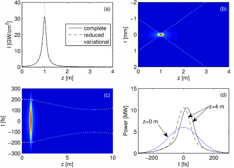
Figure 1: (a) Peak intensities of a Gaussian pulse with $P_{\rm in}=6$ MW, $w_{0}=1$ mm and $\tau_{p}=200$ fs, focused in xenon at atmospheric pressure ($f=1$ m). Solid line corresponds to the complete model Eq. (1), dashed (superimposed) line to Eq. (2), and dotted line to the variational model Eq. (3). (b) Spatial and (c) temporal dynamics of the full model. White dots reproduce the beam waist and 1/e² temporal extent computed from Eq. (3). (d) Power profiles after 4 m of propagation for the full model (solid line) and the reduced model Eq. (2) (dashed line). The blue line shows the initial pulse.

Let us then inspect regions of temporal instability. When we increase both the input power and focal length by a factor five, the variational model predicts $I_{\rm max}\simeq 6$ GW/cm², $w_{\rm min}\simeq 640~{}\mu$m and $\tau_{\rm min}\simeq 33$ fs, resulting in $k_{\perp}^{\rm max}\simeq 69$ cm^-1, $\overline{\omega}_{\rm up}\simeq 0.13$ fs^-1 and $\overline{\omega}_{\rm max}\simeq 0.071$ fs^-1. Since $\overline{\omega}_{\rm up}>\overline{\omega}_{\rm max}$, nonlinearities should thus seed MI and compression in time. This is actually confirmed by the simulations shown in Fig. 2. Compression leads to a short peak of $\sim 25$ fs duration at $z=4$ m, before MI fully breaks up the pulse temporal distribution. The modulation period is about $2\pi/\overline{\omega}_{\rm max}\sim 150$ fs, which agrees with Figs. 2(d) and (e). Note that again the minimum duration predicted by Eq. (3) occurs beyond the compression stage seen in the simulations. The numerical pulse is subject to leaks of power, which the variational approach cannot describe by preserving the input power within a Gaussian ansatz Bergé and Rasmussen (1996). However, Eq. (3) reproduces compression rates agreeing well with the numerical data. While nonlinear dispersion clearly influences the pulse dynamics by moving its temporal centroid towards positive times, we observe qualitative agreement between results obtained from Eqs. (1) and (2) [compare Figs. 2(b), (c) and 2(d), (e)].

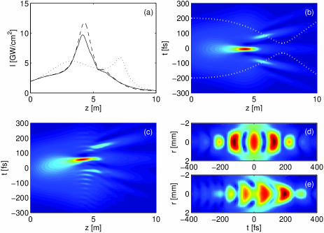
Figure 2: (a) Peak intensities of the same Gaussian pulse as in Fig. 1, but with $P_{\rm in}=30$ MW and $f=5$ m, using the same plotstyle as in Fig. 1(a). (b) Temporal on-axis dynamics obtained from Eq. (2); white dots correspond to the variational approximation. (c) Same from the complete model Eq. (1). Spatio-temporal intensity distribution at $z=8$ m showing MI from (d) the reduced model, (e) the complete model.

Figure 3 concerns the main result of this Letter. By tuning the input parameters appropriately, MI can be handled, such that only one modulation mainly affects the pulse temporal profile. Since a negative $n_{2}$ may lead to compression at distances $z>z_{\rm min}$, the pulse can then not only reach very short durations, but also keep them over long distances. The condition for this regime of optimal pulse compression is obviously $\overline{\omega}_{\rm up}\simeq\overline{\omega}_{\rm max}$. Let us examine the evolution of a Gaussian pulse, for which we reduce both initial waist, pulse duration and power to $w_{0}=0.3$ mm, $\tau_{p}=100$ fs, and $P_{\rm in}=24$ MW, respectively, to obtain $\overline{\omega}_{\rm max}\simeq 0.14$ fs^-1 and $\overline{\omega}_{\rm up}\simeq 0.17$ fs^-1. Figures 3(a) and (b) detail the pulse evolution computed from Eqs. (2) and (1), respectively. MI is weakly seeded and the 100 fs pulse undergoes three modulations, among which only the central one is amplified and compressed along further propagation down to $\sim 25$ fs. The resulting structure appears to behave like a 1D sech-soliton in time, capable of preserving high intensity and short durations over at least 50 cm. Again we observe a slight shift to the trailing part of the pulse caused by the nonlinear dispersion. At such weak intensities, we can also infer that two-photon absorption remains of small influence. It is nevertheless important to point out that, in contrast to filamentary compression in self-focusing regime Hauri et al. (2004); Skupin et al. (2006); Zaïr et al. (2007), short pulses obtained with the above compression scheme are homogeneous in radial direction. Hence, compression applies not only to the on-axis intensity profiles, but also to the pulse power profiles. Moreover, the XFROG trace shown in Fig. 3(d) indicates that the compressed pulses are nearly transform limited.

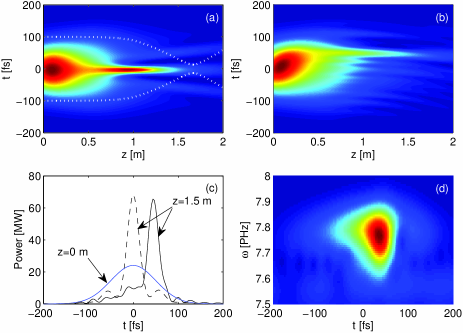
Figure 3: Dynamics of a Gaussian pulse with $P_{\rm in}=24$ MW, $w_{0}=0.3$ mm and $\tau_{p}=100$ fs, focused in xenon with $f=1$ m. (a) Temporal on-axis dynamics obtained from the reduced model; white dots correspond to variational results. (b) Same from the full model. (c) Power profiles after 1.5 m of propagation for the full model (solid line) and the reduced model (dashed line). The blue line shows the initial pulse. (d) XFROG trace at $z=1.5$ m using a $25$ fs reference pulse.

A last point concerns spectral broadening, as SPM is responsible for frequency variations $\Delta\omega\simeq k_{0}\Delta z|n_{2}|I_{\rm max}/\tau_{\rm min}$ around the focus. Spectral variations should remain confined within the narrow bandwidth of 238–249 nm (7.57–7.92 PHz), in order to preserve a negative value of $n_{2}\sim\chi^{(3)}(\omega;-\omega,\omega,\omega)$ along the optical path [see Fig. 4(b)]. Figure 4(a) confirms that the spectrum has a small bandwidth of $\Delta\omega<0.1$ PHz at half-maximum. For the simulation shown in Fig. 3, spectral wings reach the range where $n_{2}$ is not necessarily negative, but the dominant peak always remains located around the central frequency [solid line in Fig. 4(a)]. We can notice that the usual broad low-intensity supercontinuum ($\Delta\omega_{\rm SC}/\omega_{0}>1$) routinely observed from the propagation of plasma-induced filaments and caused by the mechanism of intensity clamping is missing. We indeed find $\Delta\omega_{\rm SC}/\omega_{0}<0.1$, where $\Delta\omega_{\rm SC}$ is measured at $10^{-5}$ times the maximum spectral intensity. Supercontinuum generation is thus inhibited, as the peak intensity stays at moderate values.

Figure 4: (a) On-axis normalized spectra for the pulses shown in Fig. 2(e) (dashed line) and Fig. 3(c) (solid line). The dotted line represents the spectrum of the 100 fs pulse at $z=0$. (b) Real part of the normalized nonlinear susceptibility $\chi^{(3)}$ in the degenerated case (see Ref. Junnarkar and Uesugi (2000)).

Further increase of the input power to 60 MW leads to the occurrence of strong MI and multiple pulse splitting ($\overline{\omega}_{\rm up}>\overline{\omega}_{\rm max}$, not shown here). For such high powers, however, a major part of the broadened spectrum falls into the range of multi-photon resonances below 7.57 PHz, and strong discrepancies between the solutions of Eq. (1) and Eq. (2) appear. Consequently, while it is possible in the NLS model to produce even shorter pulses $<20$ fs by simply increasing the initial peak power, dispersion of the nonlinear susceptibility prevented us from achieving shorter durations with Eq. (1). Such propagation regimes will be addressed in a future publication.

In summary, numerical simulations have highlighted the dynamics of UV pulses focused into a self-defocusing gas cell. Ultrashort optical structures can naturally be formed in (3+1)-dimensional media with negative $n_{2}$ and normal dispersion, and propagate over long ranges without experiencing a wide spectral broadening. By mixing simple analytical procedures, we proved that this new compression mechanism follows from modulational instability in time, which can be controlled to optimize the self-compression process over long distances. To end with, we find it worth emphasizing that nonlinear dispersion yielding variations in the Kerr index of at least one order of magnitude does not significantly change results compared to propagation models assuming a constant susceptibility. Here, we indeed showed that at moderate powers deviations associated with nonlinear dispersion remain limited and their qualitative effect is similar to classical pulse self-steepening in focusing media.

This work has been performed using HPC resources from GENCI-CCRT/CINES (Grant 2009-x2009106003).

References

- Alfano (2006) R. R. Alfano, ed., The Supercontinuum Laser Source: Fundamentals with Updated References (Springer-Verlag, Germany, 2006).
- Nisoli et al. (1997) M. Nisoli, S. De Silvestri, O. Svelto, R. Szipöcs, K. Ferencz, C. Spielmann, S. Sartania, and F. Krausz, Opt. Lett. 22, 522 (1997).
- Liu et al. (1999) X. Liu, L. Qian, and F. W. Wise, Opt. Lett. 24, 1777 (1999).
- Ashihara et al. (2002) S. Ashihara, J. Nishina, T. Shimura, and K. Kuroda, J. Opt. Soc. Am. B 19, 2505 (2002).
- Bache et al. (2007) M. Bache, J. Moses, and F. W. Wise, J. Opt. Soc. Am. B 24, 2752 (2007).
- Hauri et al. (2004) C. P. Hauri, W. Kornelis, F. W. Helbing, A. Heinrich, A. Couairon, A. Mysyrowicz, J. Biegert, and U. Keller, Appl. Phys. B: Lasers & Optics 79, 673 (2004).
- Skupin et al. (2006) S. Skupin, G. Stibenz, L. Bergé, F. Lederer, T. Sokollik, M. Schnürer, N. Zhavoronkov, and G. Steinmeyer, Phys. Rev. E 74, 056604 (2006).
- Zaïr et al. (2007) A. Zaïr, A. Guandalini, F. Schapper, M. Holler, J. Biegert, L. Gallmann, A. Couairon, M. Franco, A. Mysyrowicz, and U. Keller, Opt. Express 15, 5394 (2007).
- Fuji et al. (2007) T. Fuji, T. Horio, and T. Suzuki, Opt. Lett. 32, 2481 (2007).
- Théberge et al. (2006) F. Théberge, N. Aközbek, W. Liu, A. Becker, and S. L. Chin, Phys. Rev. Lett. 97, 023904 (2006).
- Trushin et al. (2007) S. A. Trushin, K. Kosma, W. Fuss, and W. E. Schmid, Opt. Lett. 32, 2432 (2007).
- Bergé and Skupin (2008) L. Bergé and S. Skupin, Opt. Lett. 33, 750 (2008).
- Lehmberg et al. (1995) R. H. Lehmberg, C. J. Pawley, A. V. Deniz, M. Klapisch, and Y. Leng, Opt. Commun. 121, 78 (1995).
- Junnarkar and Uesugi (2000) M. R. Junnarkar and N. Uesugi, Opt. Commun. 175, 447 (2000).
- Kivshar and Luther-Davies (1998) Y. S. Kivshar and B. Luther-Davies, Phys. Rep. 298, 81 (1998).
- Bergé and Rasmussen (1996) L. Bergé and J. J. Rasmussen, Phys. Plasmas 3, 824 (1996).
- Bespalov and Talanov (1966) V. I. Bespalov and V. I. Talanov, JETP Lett. 3, 307 (1966).
- Couairon and Bergé (2000) A. Couairon and L. Bergé, Phys. Plasmas 7, 193 (2000).
- Dalgarno and Kingston (1960) A. Dalgarno and A. E. Kingston, Proc. Royal Soc. London A 259, 424 (1960).