Green Modulation in Proactive Wireless Sensor Networks

Abstract

Due to unique characteristics of sensor nodes, choosing energy-efficient modulation scheme with low-complexity implementation (refereed to as green modulation) is a critical factor in the physical layer of Wireless Sensor Networks (WSNs). This paper presents (to the best of our knowledge) the first in-depth analysis of energy efficiency of various modulation schemes using realistic models in IEEE 802.15.4 standard and present state-of-the art technology, to find the best scheme in a proactive WSN over Rayleigh and Rician flat-fading channel models with path-loss. For this purpose, we describe the system model according to a pre-determined time-based process in practical sensor nodes. The present analysis also includes the effect of bandwidth and active mode duration on energy efficiency of popular modulation designs in the pass-band and Ultra-WideBand (UWB) categories. Experimental results show that among various pass-band and UWB modulation schemes, Non-Coherent M-ary Frequency Shift Keying (NC-MFSK) with small order of $M$ and On-Off Keying (OOK) have significant energy saving compared to other schemes for short range scenarios, and could be considered as realistic candidates in WSNs. In addition, NC-MFSK and OOK have the advantage of less complexity and cost in implementation than the other schemes.

I Introduction

Wireless Sensor Networks (WSNs) represent a new generation of distributed systems to support a broad range of applications; including monitoring and control, health care, tracking environmental pollution levels, and traffic coordination. A WSN consists of a large number of microsensors which are typically powered by small energy-constrained batteries. In many application scenarios, these batteries can not be replaced or recharged, making the sensor useless once battery life is over. Thus, minimizing the total energy consumption (i.e., circuits and signal transmission energies) is a critical factor in designing a WSN. Due to the unique characteristics and application requirements of sensor networks, deploying energy-efficient design guidelines in traditional wireless networks are not suited to the WSNs. In fact, since the output transmission energy is dependent to the distance between transmitter and receiver, long distance wireless communication systems use efficient protocols (emphasizing on modulation schemes) to minimize the output transmission energy. In these systems, the energy consumed by circuits is ignored. However, typical WSNs assume that sensor nodes are densely deployed which means distance between sensor nodes is normally short compared to the traditional wireless systems. Thus, the circuit energy consumption in a WSN is comparable to the output transmission energy. For energy-constrained WSNs, on the other hand, the data rates are usually low. Thus, using complicated signal processing techniques (e.g., high order M-ary modulation and complex detection) are not desirable for low-power WSNs.

Several energy-efficient approaches have been investigated for different layers of a WSN [2, 3, 4, 5, 6]. Central to the study of energy-efficient techniques in physical layer of a WSN is modulation. Since, achieving all requirements (e.g., minimum energy consumption, maximum bandwidth efficiency, high system performance and low complexity) is a complex task in a WSN, and due to the power limitation in sensor nodes, the choice of a proper modulation scheme is a main challenge in designing a WSN. Taking this into account, an energy-efficient modulation scheme should be simple enough to be implemented by state-of-the-art low-power technology, but still robust enough to provide the desired service. In addition, since sensor nodes frequently switch from sleep mode to active mode, modulation circuits should have fast start-up times. We refer to these low-energy consumption schemes as green modulations. In recent years, several energy-efficient modulation schemes have been studied in WSNs [4, 5, 6, 7, 8, 9]. Broadly, they can be divided into pass-band and Ultra-WideBand (UWB) modulation schemes. Pass-band modulation schemes such as M-ary Frequency Shift Keying (MFSK), M-ary Quadrature Amplitude Modulation (MQAM) and M-ary Phase Shift Keying (MPSK) use sinusoidal carrier signal for modulation. The complexity of receiver circuitry in traditional M-ary modulation schemes (e.g., MQAM and MPSK) makes their implementation on WSNs rather costly despite their great performance, e.g., Bit-Error-Rate (BER). In addition, they require Digital-to-Analog Converters (DACs) and mixers which are the most power intensive components at the receiver [10]. Ultra-wideband known as digital pulse wireless is a very short-range wireless technology (typically for 10 meters distance or less [11]) for transmitting data over a wide spectrum. UWB modulation schemes such as Pulse Position Modulation (PPM) and On-Off Keying (OOK) require no sinusoidal carrier signal for modulation. The main advantages of UWB modulation schemes are their immunity to multipath, very low transmission power and simple transceiver circuity.

Several energy-efficient modulation schemes have been investigated in physical layer of WSNs [7, 5, 12, 8, 6, 4, 13, 14, 15]. Tang et al. [5] compare the battery power efficiency of PPM and FSK schemes in a WSN without considering the effect of bandwidth and active mode period. Under the assumption of the non-linear battery model, reference [5] shows that FSK is more power-efficient than PPM in sparse WSNs, while PPM may outperform FSK in dense WSNs. References [6] and [8] compare the battery power efficiency of PPM and OOK based on the exact BER and the cutoff rate for WSNs with path-loss Additive White Gaussian Noise (AWGN) channels. Reference [15] investigates the energy efficiency of a centralized WSN with adaptive MQAM scheme. Most of the pioneering work on energy-efficient modulation (e.g. [5, 6, 7, 8]) has only focused on minimizing the average energy consumption of transmitting one bit without considering the effect of bandwidth and transmission time duration. In a practical WSN however, it is shown that minimizing the total energy consumption depends strongly on active mode duration and the channel bandwidth. Reference [4] addresses this problem only for MFSK and MQAM for AWGN channel model with path-loss, and shows that MQAM is more energy-efficient than MFSK for short-range applications. In addition, some literature (e.g., [5]) have compared the energy consumption of pass-band modulation schemes with that of UWB ones without considering the point that the channel bandwidth of UWB schemes is much wider than that of pass-band ones. Thus, due to the dependency of total energy consumption on bandwidth, this kind of comparison would not meaningful. Furthermore deploying adaptive modulation schemes [15] are not practically feasible in WSNs, as they require some additional system complexity as well as channel state information fed back from sink node to sensor node.

In this paper, we analyze in-depth the energy efficiency of various modulation schemes considering the effect of channel bandwidth and active mode duration to find the green modulation in a proactive wireless sensor network. For this purpose, we describe the system model according to a pre-determined time-based process in practical sensor nodes. Also, new analysis results for comparative evaluation of popular modulation designs in the pass-band and UWB categories are introduced according to realistic parameters in IEEE 802.15.4 standard [16]. We start the energy efficiency analysis based on Rayleigh flat-fading channel model with path-loss which is a feasible model in static WSNs [5, 6]. Then, we evaluate numerically the energy efficiency of pass-band modulation schemes operating over the more general Rician model which includes a strong direct Line-Of Sight (LOS) path. Experimental results show that among various pass-band modulation schemes, non-coherent MFSK is a realistic option in short to moderate range WSNs, since it has the advantage of less complexity and cost in implementation than MQAM and Offset Quadrature Phase Shift Keying (OQPSK) used in Zigbee/IEEE 802.15.4 protocols, and has less total energy consumption. In addition, since for typical energy-constrained WSNs, data transmission rates are usually low, using small order M-ary FSK schemes are desirable. Furthermore, simulation results show that OOK has less total energy consumption in very short WSN applications, along with the advantage of less complexity and cost in implementation than M-PPM.

The rest of the paper is organized as follows. In Section II, the proactive system model and assumptions are described. A comprehensive analysis of the energy efficiency for various pass-band and UWB modulation schemes is presented in Sections III and IV. Section V provides some numerical evaluations using realistic models to confirm our analysis. Also, some design guidelines for green modulation in practical WSN applications are presented. Finally in Section VI, an overview of the results and conclusions is presented.

II System Model and Assumptions

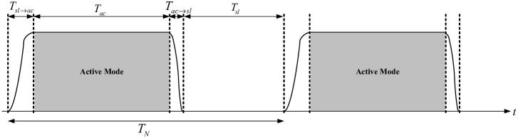
Figure 1: A practical multi-mode operation in a proactive WSN.

In this work, we consider a proactive wireless sensor system, in which a sensor node samples continuously the environment and transmits the equal amount of data per time unit to a designated sink node. This proactive system is the case of many environmental applications such as sensing temperature, solar radiation and level of contamination [17]. The sensor and sink nodes synchronize with each other and work in a real time-based process as depicted in Fig 1. During active mode duration $T_{ac}$, the analog signal sensed by the sensor is first digitized by an Analog-to-Digital Converter (ADC), and an $N$-bit message sequence $(a_{1},a_{2},...,a_{N})$ is generated, where $N$ is assumed to be fixed, and $a_{i}\in\{0,1\}$, $i=1,2,...,N$. The above stream is modulated using a pre-determined modulation scheme and then transmitted to the sink node. Finally, sensor node back to sleep mode, and all the circuits of the transceiver is shutdown in sleep mode duration $T_{sl}$ for energy saving. We denote $T_{tr}$ as the transient mode duration consisting of the switching time from sleep mode to active mode (i.e., $T_{sl\rightarrow ac}$) plus the switching time from active mode to sleep mode (i.e., $T_{ac\rightarrow sl}$), where $T_{ac\rightarrow sl}$ is assumed to be negligible. When a sensor switches from sleep mode to active mode to send data, a significant amount of power is consumed for starting up the transmitter, while the power consumption during $T_{ac\rightarrow sl}$ is negligible. Thus, choosing an efficient-modulation scheme with fast start-up circuits is desirable in designing WSNs. Under the above considerations, the sensor node has $N$ bits to transmit during $0\leq T_{ac}\leq T_{N}-T_{tr}$, where $T_{N}\triangleq T_{tr}+T_{ac}+T_{sl}$ is assumed to be fixed for each modulation scheme, and $T_{tr}\approx T_{sl\rightarrow ac}$. Note that $T_{ac}$ is a critical factor in choosing an efficient modulation scheme, as it directly affects the total energy consumption as we will see later.

Since sensor nodes in a typical WSN are densely deployed, the circuits power consumption $\mathcal{P}_{c}\triangleq\mathcal{P}_{ct}+\mathcal{P}_{cr}$ is comparable to the output transmit power consumption denoted by $\mathcal{P}_{t}$, where $\mathcal{P}_{ct}$ and $\mathcal{P}_{cr}$ represent the circuit power consumptions of sensor and sink nodes, respectively. Taking these into account, the total energy consumption in the active mode period, denoted by $\mathcal{E}_{ac}$, is given by $\mathcal{E}_{ac}=(\mathcal{P}_{c}+\mathcal{P}_{t})T_{ac}$, where $T_{ac}$ is a function of $N$ and the channel bandwidth as we will show in Section III. Also, the energy consumption in sleep mode duration, denoted by $\mathcal{E}_{sl}$, is given by $\mathcal{E}_{sl}=\mathcal{P}_{sl}T_{sl}$, where $\mathcal{P}_{sl}$ is the corresponding power consumption. It is worth mentioning that during sleep mode period, the leakage current coming from CMOS circuits is a dominant factor in $\mathcal{P}_{sl}$. Clearly, higher sleep mode duration increases energy consumption $\mathcal{E}_{sl}$ due to increasing leakage current as well as $T_{sl}$. Present state-of-the art technology aims to keep a low sleep mode leakage current no longer than the battery leakage current, which results in $\mathcal{P}_{sl}$ much smaller than the power consumption in active mode [18]. For this reason, we assume that $\mathcal{P}_{sl}\approx 0$. As a result, the energy efficiency, referred to as the performance metric of the proposed WSN, can be defined as the total energy consumption in each period $T_{N}$ correspond to $N$-bit message as follows:

$$\mathcal{E}_{N}\approx(\mathcal{P}_{c}+\mathcal{P}_{t})T_{ac}+\mathcal{P}_{tr}T_{tr},$$ (1)

where $\mathcal{P}_{tr}$ is the circuit power consumption during transient mode period. We use (1) to investigate and compare the energy efficiency of various modulation schemes.

Channel Model: The choice of low transmission power in WSNs represents several consequences for channel modeling. It is shown by Friis [19] that a low transmission power implies a small range. On the other hand, for short-range transmission scenarios, the root mean square (rms) delay spread is in the range of nanoseconds [11] (and picoseconds for UWB applications [20]) which is small compared to symbol durations for modulation schemes. For instance, the channel bandwidth and the correspond symbol duration considered in IEEE 802.15.4 standard are $B=62.5$ KHz and $T_{s}=16~{}\mu$s, respectively [16, p. 49], while the rms delay spread in indoor environments are in the range of 70-150 ns [21]. Thus, it is reasonable to expect a flat-fading channel model for WSNs. Under the above considerations, the channel model between the sensor and sink nodes is assumed to be Rayleigh flat-fading with path-loss, which is a feasible model in static WSNs [5, 6]. We denote the fading channel coefficient correspond to a transmitted symbol $i$ as $h_{i}$, where the amplitude $\big{|}h_{i}\big{|}$ is Rayleigh distributed with probability density function (pdf) given according to $f_{|h_{i}|}(r)=\frac{2r}{\Omega}e^{-\frac{r^{2}}{\Omega}},~{}r\geq 0$, where $\Omega\triangleq\mathbb{E}\left[|h_{i}|^{2}\right]$ (pp. 767-768 of [22]). This results $|h_{i}|^{2}$ being chi-square distributed with 2 degrees of freedom, where $f_{|h_{i}|^{2}}(r)=\frac{1}{\Omega}e^{\frac{-r}{\Omega}}$.

To model the path-loss of a link in a distance $d$, let denote $\mathcal{P}_{t}$ and $\mathcal{P}_{r}$ as the transmitted and the received signal powers, respectively. For a $\eta^{th}$-power path-loss channel, the channel gain factor is given by $\mathcal{L}_{d}\triangleq\frac{\mathcal{P}_{t}}{\mathcal{P}_{r}}=M_{l}d^{\eta}\mathcal{L}_{1}$, where $M_{l}$ is the gain margin which accounts for the effects of hardware process variations, background noise and $\mathcal{L}_{1}\triangleq\frac{(4\pi)^{2}}{\mathcal{G}_{t}\mathcal{G}_{r}\lambda^{2}}$ is the gain factor at $d=1$ meter which is specified by the transmitter and receiver antenna gains $\mathcal{G}_{t}$ and $\mathcal{G}_{r}$, and wavelength $\lambda$ (e.g., [4], [6] and [23]). As a result, when both fading and path-loss are considered, the instantaneous channel coefficient becomes $G_{i}\triangleq\frac{h_{i}}{\sqrt{\mathcal{L}_{d}}}$. Denoting $x_{i}(t)$ as the transmitted signal with energy $\mathcal{E}_{t}$, the received signal at sink node is given by $y_{i}(t)=G_{i}x_{i}(t)+n_{i}(t)$, where $n_{i}(t)$ is AWGN with two-sided power spectral density given by $\frac{N_{0}}{2}$. Under the above considerations, the instantaneous Signal-to-Noise Ratio (SNR), denoted by $\gamma_{i}$, correspond to an arbitrarily symbol $i$ can be computed as $\gamma_{i}=\frac{|G_{i}|^{2}\mathcal{E}_{t}}{N_{0}}$. Under the assumption of Rayleigh fading channel model, $\gamma_{i}$ is chi-square distributed with 2 degrees of freedom, with pdf $f_{\gamma}(\gamma_{i})=\frac{1}{\bar{\gamma}}\exp\left(-\frac{\gamma_{i}}{\bar{\gamma}}\right)$, where $\bar{\gamma}\triangleq\mathbb{E}[|G_{i}|^{2}]\frac{\mathcal{E}_{t}}{N_{0}}=\frac{\Omega}{\mathcal{L}_{d}}\frac{\mathcal{E}_{t}}{N_{0}}$ denotes the average received SNR.

III Energy Consumption Analysis of Pass-band Modulation Schemes

Pass-band modulation schemes such as MFSK, MQAM and OQPSK use sinusoidal carrier signal for modulation. In the following, we investigate three popular carrier-based modulation schemes from energy and bandwidth efficiency points of view over Rayleigh fading channel model with path-loss.

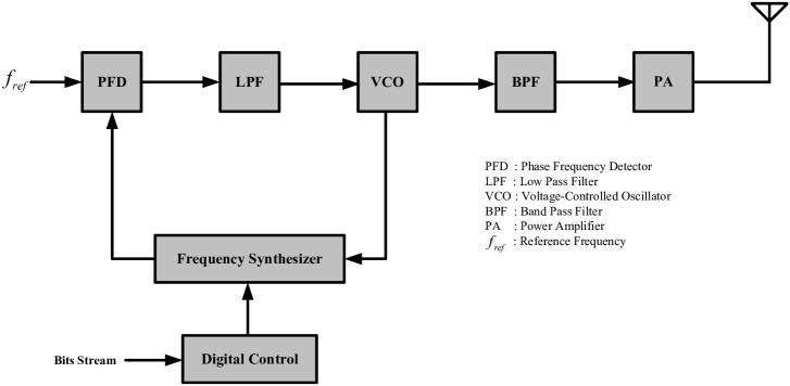
Figure 2: General block diagram of an MFSK modulator.

M-ary FSK: Let assume the bits stream $(a_{1},...,a_{N})$ is considered as modulating signals in an $M$-ary FSK modulation scheme, where $M$ orthogonal carriers can be mapped into $b\triangleq\log_{2}M$ bits. The main advantage of this M-ary orthogonal signaling is that received signals do not interfere with each other in the process of detection at the receiver. An MFSK modulator benefits from the advantage of using the Direct Digital Modulation (DDM) approach, i.e., it does not need mixer and DAC which are used for MQAM and MPSK (see Fig. 2). In fact, MFSK modulation is usually implemented digitally inside the frequency synthesizer. This property makes MFSK has faster start-up time than other pass-band schemes [10]. The output of the frequency synthesizer can be frequency modulated and controlled simply by $b$ bits in the input of a “digital control” block. The modulated signal is then filtered again, amplified by the Power Amplifier (PA), and finally transmitted to the wireless channel.

Denoting $\mathcal{E}^{FS}_{t}$ as the MFSK transmit energy per symbol with symbol duration $T^{FS}_{s}$, the MFSK transmitted signal is given by $x^{FS}_{i}(t)=\sqrt{\frac{2\mathcal{E}^{FS}_{t}}{T^{FS}_{s}}}\cos(2\pi(f_{0}+i.\Delta f)t),~{}i=0,1,...M-1$, where $f_{0}$ is the first carrier frequency in the MFSK modulator and $\Delta f$ is the minimum carrier separation which is equal to $\frac{1}{2T^{FS}_{s}}$ for coherent FSK and $\frac{1}{T^{FS}_{s}}$ for non-coherent FSK [24, p. 114]. Thus, the channel bandwidth $B$ is obtained as $B\approx M\times\Delta f$, where $B$ is assumed to be fixed for all pass-band modulation schemes. Denoting $B^{FS}_{eff}$ as the bandwidth efficiency of MFSK (in units of bits/s/Hz) defined as the ratio of data rate $R^{FS}=\frac{b}{T^{FS}_{s}}$ (bits/sec) to the channel bandwidth, we have $B^{FS}_{eff}\triangleq\frac{R^{FS}}{B}=\frac{\zeta\log_{2}M}{M}$, where $\zeta=2$ for coherent and $\zeta=1$ for non-coherent FSK. It is observed that increasing constellation size $M$ leads to decrease in the bandwidth efficiency in MFSK. However, the effect of increasing $M$ on the energy efficiency should be considered as well. To address this problem, we first derive the relationship between $M$ and the active mode duration $T^{FS}_{ac}$. Noting that during each symbol period $T^{FS}_{s}$, we have $b$ bits, it is concluded that

$$T^{FS}_{ac}=\dfrac{N}{b}T^{FS}_{s}=\dfrac{MN}{\zeta B\log_{2}M}.$$ (2)

Recalling that $B$ and $N$ are fixed, increasing $M$ results in increasing in $T^{FS}_{ac}$. However, as illustrated in Fig. 1, the maximum value for $T^{FS}_{ac}$ is bounded by $T_{N}-T^{FS}_{tr}$. Thus, the maximum constellation size $M$, denoted by $M_{max}\triangleq 2^{b_{max}}$, for MFSK is calculated by the non-linear equation $\frac{2^{b_{max}}}{\zeta b_{max}}=\frac{B}{N}(T_{N}-T^{FS}_{tr})$.

At the receiver side, the received MFSK signal can be detected coherently to provide optimum performance. However, the MFSK coherent detection requires the receiver to obtain a precise frequency and carrier phase reference for each of the transmitted orthogonal carriers. For large $M$, this would increase the complexity of detector which makes a coherent MFSK receiver very difficult to implement. Due to the above considerations, most practical MFSK receivers use non-coherent detectors. The optimum Non-Coherent MFSK (NC-MFSK) consists of a bank of $M$ matched filters, each followed by an envelop (or square-law) detector [25]. At the sampling times $t=\ell T^{FS}_{s}$, a maximum-likelihood makes decision based on the largest filter output. It is worth mentioning that using an envelope detector for demodulation avoids the use of power-intensive active analogue components such as mixer in coherent detectors.

Now, we are ready to derive the total energy consumption of a NC-MFSK. We first derive $\mathcal{E}^{FS}_{t}$, the transmit energy per symbol, in terms of a given average Symbol Error Rate (SER) denoted by $P_{s}$. The average SER of a NC-MFSK is given by $P_{s}=\int_{0}^{\infty}P_{s}(\gamma_{i})f_{\gamma}(\gamma_{i})d\gamma_{i}$, where $P_{s}(\gamma_{i})$ namely the SER conditioned upon $\gamma_{i}$, is obtained as $P_{s}(\gamma_{i})=\int_{0}^{\infty}uI_{0}(\sqrt{2\gamma_{i}u})\left[1-\left(1-e^{-\frac{u^{2}}{2}}\right)^{M-1}\right]e^{-\frac{u^{2}+2\gamma_{i}}{2}}du$, where $I_{0}(x)$ is the zeroth order modified Bessel function [26, 5]. It is shown in [5, Lemma 2] that the above $P_{s}$ is upper bounded by $P_{s}\leq 1-\left(1-\frac{1}{2+\bar{\gamma}^{FS}}\right)^{M-1}$, where $\bar{\gamma}^{FS}=\frac{\Omega}{\mathcal{L}_{d}}\frac{\mathcal{E}^{FS}_{t}}{N_{0}}$. As a result, the transmit energy consumption per each symbol is obtained as $\mathcal{E}^{FS}_{t}\triangleq\mathcal{P}^{FS}_{t}T^{FS}_{s}\leq\left[\left(1-(1-P_{s})^{\frac{1}{M-1}}\right)^{-1}-2\right]\frac{\mathcal{L}_{d}N_{0}}{\Omega}$. Since, it aims to obtain the maximum energy consumption, we approximate the above upper bound as an equality. Using (2), the output energy consumption of transmitting $N$ bits during $T^{FS}_{ac}$ is computed as

$$\mathcal{P}^{FS}_{t}T^{FS}_{ac}=\dfrac{T^{FS}_{ac}}{T^{FS}_{s}}\mathcal{E}^{FS}_{t}\approx\left[\left(1-(1-P_{s})^{\frac{1}{M-1}}\right)^{-1}-2\right]\dfrac{\mathcal{L}_{d}N_{0}}{\Omega}\dfrac{N}{\log_{2}M},$$ (3)

which is a monotonically increasing functions of $M$ for every value of $P_{s}$ and $d$. In addition, the energy consumption of the sensor and the sink circuitry during $T^{FS}_{ac}$ is computed as $(\mathcal{P}^{FS}_{ct}+\mathcal{P}^{FS}_{cr})T^{FS}_{ac}$. For the sensor node with MFSK, we denote the power consumption of frequency synthesizer, filters and power amplifier as $\mathcal{P}^{FS}_{Sy}$, $\mathcal{P}^{FS}_{Filt}$ and $\mathcal{P}^{FS}_{Amp}$, respectively. In this case, $\mathcal{P}^{FS}_{ct}=\mathcal{P}^{FS}_{Sy}+\mathcal{P}^{FS}_{Filt}+\mathcal{P}^{FS}_{Amp}$. It is shown that the relationship between $\mathcal{P}^{FS}_{Amp}$ and the transmission power of an MFSK signal is $\mathcal{P}^{FS}_{Amp}=\alpha^{FS}\mathcal{P}^{FS}_{t}$, where $\alpha^{FS}$ is determined based on type of power amplifier. For instance for a class B power amplifier, $\alpha^{FS}=0.33$ [4], [5]. For the power consumption of the sink circuity, we use the fact that each branch in NC-MFSK demodulator consists of band pass filters followed by an envelop detector. Also, we assume that the sink node uses a Low-Noise Amplifier (LNA) which is generally placed at the front-end of a RF receiver circuit, an Intermediate-Frequency Amplifier (IFA), and an ADC unit, regardless of type of deployed pass-band modulation scheme. Thus, denoting $\mathcal{P}^{FS}_{LNA}$, $\mathcal{P}^{FS}_{Filr}$, $\mathcal{P}^{FS}_{ED}$, $\mathcal{P}^{FS}_{IFA}$ and $\mathcal{P}^{FS}_{ADC}$ as the power consumption of LNA, filters, envelop detector, IF amplifier and ADC, respectively, the power consumption of the sink circuitry can be obtained as $\mathcal{P}^{FS}_{cr}=\mathcal{P}^{FS}_{LNA}+M\times(\mathcal{P}^{FS}_{Filr}+\mathcal{P}^{FS}_{ED})+\mathcal{P}^{FS}_{IFA}+\mathcal{P}^{FS}_{ADC}$. In addition, it is shown that the power consumption during transition mode period $T^{FS}_{tr}$ is governed by the frequency synthesizer [7]. Taking this into account, the energy consumption during $T^{FS}_{tr}$ is obtained as $\mathcal{P}^{FS}_{tr}T^{FS}_{tr}=1.75\mathcal{P}^{FS}_{Sy}T^{FS}_{tr}$ [11]. As a result, the total energy consumption of a NC-MFSK scheme for transmitting $N$ bits in each period $T_{N}$, under the constraint $M\leq M_{max}$ and for a given $P_{s}$ is obtained as

$$\mathcal{E}^{FS}_{N}=(1+\alpha^{FS})\left[\left(1-(1-P_{s})^{\frac{1}{M-1}}\right)^{-1}-2\right]\dfrac{\mathcal{L}_{d}N_{0}}{\Omega}\dfrac{N}{\log_{2}M}+(\mathcal{P}^{FS}_{c}-\mathcal{P}^{FS}_{Amp})\dfrac{MN}{B\log_{2}M}+1.75\mathcal{P}^{FS}_{Sy}T^{FS}_{tr}.$$ (4)

M-ary QAM: For $M$-ary QAM with square constellation, each $b=\log_{2}M$ bits of the message is mapped to a complex symbol $S_{i}$, $i=0,1,...,M-1$, where the constellation size $M$ is a power of 4. Assuming raised-cosine filter (with a proper filter roll-off) is used for pulse shaping, the channel bandwidth of MQAM is determined as $B\approx\frac{1}{2T^{QA}_{s}}$, where $T^{QA}_{s}$ represents the MQAM symbol duration. Using the data rate $R^{QA}=\frac{b}{T^{QA}_{s}}$ (bits/sec), the bandwidth efficiency of MQAM is obtained as $B^{QA}_{eff}\triangleq\frac{R^{QA}}{B}=2\log_{2}M~{}\textrm{(bits/s/Hz)}$. It is observed that $B^{QA}_{eff}$ is a logarithmically increasing function of $M$. To address the effect of increasing $M$ on the energy efficiency, we first derive the relationship between $M$ and active mode duration $T^{QA}_{ac}$. Recalling that during period $T^{QA}_{s}$, we have $b$ bits, it is concluded that

$$T^{QA}_{ac}=\dfrac{N}{b}T^{QA}_{s}=\dfrac{N}{2B\log_{2}M}.$$ (5)

We can see from (5) that increasing $M$ results in decreasing in $T^{QA}_{ac}$. Also compared to (2), it is concluded that $\frac{T^{QA}_{ac}}{T^{FS}_{ac}}=\frac{1}{M}<1$. To obtain the transmit energy consumption $\mathcal{P}^{QA}_{t}T^{QA}_{ac}$, we use the similar arguments as MFSK. The SER conditioned upon $\gamma_{i}$ of a coherent MQAM is given by [27, pp. 226]

$$P_{s}(\gamma_{i}) = 4\left(1-\dfrac{1}{\sqrt{M}}\right)Q\left(\sqrt{\dfrac{3\gamma_{i}}{M-1}}\right)-4\left(1-\dfrac{1}{\sqrt{M}}\right)^{2}Q^{2}\left(\sqrt{\dfrac{3\gamma_{i}}{M-1}}\right)$$ (6)

$$\leq 4\left(1-\dfrac{1}{\sqrt{M}}\right)Q\left(\sqrt{\dfrac{3\gamma_{i}}{M-1}}\right)$$ (7)

$$\stackrel{{\scriptstyle(a)}}{{\leq}} 2\left(1-\dfrac{1}{\sqrt{M}}\right)\exp\left(-\dfrac{3\gamma_{i}}{2(M-1)}\right),$$ (8)

where $Q(x)\triangleq\frac{1}{\sqrt{2\pi}}\int_{x}^{\infty}e^{-u^{2}/2}du$ is the area under the tail of the Gaussian distribution, and $(a)$ comes from $Q(x)\leq\frac{1}{2}e^{-x^{2}/2}$, $x>0$. Thus, the average SER of a coherent MQAM is upper bounded by

$$P_{s} = \int_{0}^{\infty}P_{s}(\gamma_{i})f_{\gamma}(\gamma_{i})d\gamma_{i}\leq\dfrac{2}{\bar{\gamma}^{QA}}\left(1-\dfrac{1}{\sqrt{M}}\right)\int_{0}^{\infty}e^{-\frac{3\gamma_{i}}{2(M-1)}}.e^{-\frac{\gamma_{i}}{\bar{\gamma}^{QA}}}d\gamma_{i}$$ (9)

$$= \dfrac{4(M-1)}{3\bar{\gamma}^{QA}+2(M-1)}\left(1-\dfrac{1}{\sqrt{M}}\right),$$ (10)

where $\bar{\gamma}^{QA}=\frac{\Omega}{\mathcal{L}_{d}}\frac{\mathcal{E}^{QA}_{t}}{N_{0}}$ denotes the average received SNR with energy per symbol $\mathcal{E}^{QA}_{t}$. As a result,

$$\mathcal{E}^{QA}_{t}\triangleq\mathcal{P}^{QA}_{t}T^{QA}_{s}\leq\dfrac{2(M-1)}{3}\left[2\left(1-\dfrac{1}{\sqrt{M}}\right)\dfrac{1}{P_{s}}-1\right]\dfrac{\mathcal{L}_{d}N_{0}}{\Omega}.$$ (11)

With a similar argument as MFSK and by approximating the above upper bound as an equality, the energy consumption of transmitting $N$ bits during active mode period is computed as

$$\mathcal{P}^{QA}_{t}T^{QA}_{ac}=\dfrac{T^{QA}_{ac}}{T^{QA}_{s}}\mathcal{E}^{QA}_{t}\approx\dfrac{2(M-1)}{3}\left[2\left(1-\dfrac{1}{\sqrt{M}}\right)\dfrac{1}{P_{s}}-1\right]\dfrac{\mathcal{L}_{d}N_{0}}{\Omega}\dfrac{N}{\log_{2}M},$$ (12)

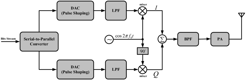
Figure 3: General block diagram of an MQAM modulator.

which is a monotonically increasing functions of $M$ for every value of $P_{s}$ and $d$. The energy consumption of the sensor and sink circuitry during active mode period $T^{QA}_{ac}$ for MQAM scheme is computed as $(\mathcal{P}^{QA}_{ct}+\mathcal{P}^{QA}_{cr})T^{QA}_{ac}$. According to Fig. 3, for the sensor node with MQAM, $\mathcal{P}^{QA}_{ct}=\mathcal{P}^{QA}_{DAC}+\mathcal{P}^{QA}_{FS}+\mathcal{P}^{QA}_{Mix}+\mathcal{P}^{QA}_{Filt}+\mathcal{P}^{QA}_{Amp}$, where $\mathcal{P}^{QA}_{DAC}$ and $\mathcal{P}^{QA}_{Mix}$ denote the power consumption of DAC and mixer. It is shown that the relationship between $\mathcal{P}^{QA}_{Amp}$ and the transmission power $\mathcal{P}^{QA}_{t}$ is given by $\mathcal{P}^{QA}_{Amp}=\alpha^{QA}\mathcal{P}^{QA}_{t}$, where $\alpha^{QA}=\frac{\xi}{\vartheta}-1$ with $\xi=3\frac{\sqrt{M}-1}{\sqrt{M}+1}$ and $\vartheta=0.35$ [4]. In addition, the power consumption of the sink circuitry with coherent MQAM can be obtained as $\mathcal{P}^{QA}_{cr}=\mathcal{P}^{QA}_{LNA}+\mathcal{P}^{QA}_{Mix}+\mathcal{P}^{QA}_{Sy}+\mathcal{P}^{QA}_{Filr}+\mathcal{P}^{QA}_{IFA}+\mathcal{P}^{QA}_{ADC}$. Also, with a similar argument as MFSK, we assume that the circuit power consumption during transition mode period $T^{QA}_{tr}$ is governed by the frequency synthesizer. As a result, the total energy consumption of a coherent MQAM system for transmitting $N$ bits in each period $T_{N}$ is obtained as

$$\mathcal{E}^{QA}_{N} = (1+\alpha^{QA})\dfrac{2(M-1)}{3}\left[2\left(1-\dfrac{1}{\sqrt{M}}\right)\dfrac{1}{P_{s}}-1\right]\dfrac{\mathcal{L}_{d}N_{0}}{\Omega}\dfrac{N}{\log_{2}M}+$$ (13)

$$(\mathcal{P}^{QA}_{c}-\mathcal{P}^{QA}_{Amp})\dfrac{N}{2B\log_{2}M}+2\mathcal{P}^{QA}_{Sy}T^{QA}_{tr}.$$

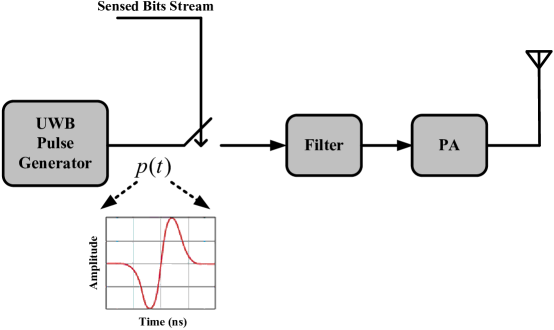
Figure 4: Block diagram of an OOK transmitter with Gaussian monocycle $p(t)$ with duration $T_{p}$.

Offset-QPSK: OQPSK referred to as staggered QPSK is used in IEEE 802.15.4 standard which is the industry standard for WSNs. The structure of an OQPSK modulator is the same as an QPSK modulator except that the in-phase (or I-channel) and the quadrature-phase (or Q-channel) pulse trains are staggered. Since OQPSK differs from QPSK only by a delay in the Q-channel signal, its error performance on a linear AWGN channel with ideal coherent detection at the receiver is the same as that of QPSK [27]. For this configuration, a coherent phase reference must be available at the receiver. However, coherent detection can be costly and increases implementation complexity due to deriving a reference carrier signal in the demodulator. On the other hand, since for OQPSK the information is carried in the phase of the carrier, and noting that non-coherent receivers are designed to ignore this phase, non-coherent detection can not be employed with OQPSK modulation. A popular technique which surpasses utilizing a coherent phase reference is to use differential encoding before classical OQPSK modulator (see [28, Fig. 4]). This is called Differential Offset QPSK (DOQPSK). In this case, the sensed data stream $(a_{1},...,a_{N})$ is first differentially encoded twice at the sensor node such that it is the change from one bit to the next using $\tilde{a}_{n}=a_{n}\oplus\tilde{a}_{n-1}$, where $\oplus$ denotes addition modulo 2. Then, the encoded bit stream is entered to the classical OQPSK modulator. For the above configuration, the channel bandwidth and the data rate are determined by $B\approx\frac{1}{T^{OQ}_{s}}$ and $R^{OQ}=\frac{2}{T^{OQ}_{s}}$ (bits/sec), respectively. As a result, the bandwidth efficiency of OQPSK is obtained as $B^{OQ}_{eff}\triangleq\frac{R^{OQ}}{B}=2$ (bits/s/Hz), which is the same as that of DOQPSK. Since during each symbol period $T^{OQ}_{s}$, we have $2$ bits, it is concluded that $T^{OQ}_{ac}=\frac{N}{2}T^{OQ}_{s}=\frac{N}{2B}$. Compared to (2) and (5), we have $T^{QA}_{ac}<T^{OQ}_{ac}<T^{FS}_{ac}$. To determine the transmit energy consumption of differential OQPSK scheme, denoted by $\mathcal{P}^{OQ}_{t}T^{OQ}_{ac}$, one would derive $\mathcal{E}^{OQ}_{t}$ in terms of SER. The SER conditioned upon $\gamma_{i}$ of differential OQPSK for two-bits observation interval is upper bounded by [29]

$$P_{s}(\gamma_{i}) \leq 1-Q_{1}\left(\sqrt{\dfrac{2+\sqrt{2}}{4}\gamma_{i}},\sqrt{\dfrac{2-\sqrt{2}}{4}\gamma_{i}}\right)+Q_{1}\left(\sqrt{\dfrac{2-\sqrt{2}}{4}\gamma_{i}},\sqrt{\dfrac{2+\sqrt{2}}{4}\gamma_{i}}\right)$$ (14)

$$\lesssim \sqrt{\dfrac{1+\sqrt{2}}{2}}\textrm{erfc}\left(\sqrt{\dfrac{2-\sqrt{2}}{4}\gamma_{i}}\right)\stackrel{{\scriptstyle(a)}}{{\leq}}\sqrt{\dfrac{1+\sqrt{2}}{2}}e^{-\frac{2-\sqrt{2}}{4}\gamma_{i}},$$ (15)

where $Q_{1}(\alpha,\beta)$ is the first-order Marcum Q-function [30] defined as $Q_{1}(\alpha,\beta)\triangleq\int_{\beta}^{\infty}xI_{0}(\alpha x)e^{-\frac{x^{2}+\alpha^{2}}{2}}dx$, and $\textrm{erfc}(x)\triangleq\frac{2}{\sqrt{\pi}}\int_{x}^{\infty}e^{-u^{2}}du$ is the complementary error function. In the above inequalities, $(a)$ follows from $\textrm{erfc}(x)\leq e^{-x^{2}}$. Thus, the average SER of differential OQPSK is upper bounded by

$$P_{s} = \int_{0}^{\infty}P_{s}(\gamma_{i})f_{\gamma}(\gamma_{i})d\gamma_{i}\leq\sqrt{\dfrac{1+\sqrt{2}}{2}}\dfrac{1}{\bar{\gamma}^{OQ}}\int_{0}^{\infty}\exp\left[-\left(\dfrac{2-\sqrt{2}}{4}+\dfrac{1}{\bar{\gamma}^{OQ}}\right)\gamma_{i}\right]d\gamma_{i}$$ (16)

$$= \sqrt{\dfrac{1+\sqrt{2}}{2}}\dfrac{4}{(2-\sqrt{2})\bar{\gamma}^{OQ}+4},$$ (17)

where $\bar{\gamma}^{OQ}=\frac{\Omega}{\mathcal{L}_{d}}\frac{\mathcal{E}^{OQ}_{t}}{N_{0}}$. Approximating the above upper bound as an equality, the transmit energy consumption per each symbol for a given $P_{s}$ is obtained as $\mathcal{E}^{OQ}_{t}\triangleq\mathcal{P}^{OQ}_{t}T^{OQ}_{s}\approx\left[\frac{1}{2-\sqrt{2}}\left(\frac{4}{P_{s}}\sqrt{\frac{1+\sqrt{2}}{2}}-4\right)\right]\frac{\mathcal{L}_{d}N_{0}}{\Omega}$. Thus, the energy consumption of transmitting $N$ bits during active mode is computed as

$$\mathcal{P}^{OQ}_{t}T^{OQ}_{ac}=\dfrac{T^{OQ}_{ac}}{T^{OQ}_{s}}\mathcal{E}^{OQ}_{t}\approx\left[\dfrac{1}{2-\sqrt{2}}\left(\dfrac{4}{P_{s}}\sqrt{\dfrac{1+\sqrt{2}}{2}}-4\right)\right]\dfrac{\mathcal{L}_{d}N_{0}}{\Omega}\dfrac{N}{2}.$$ (18)

The energy consumption of the sensor and the sink circuitry during active mode period $T^{OQ}_{ac}$ for differential OQPSK is computed as $(\mathcal{P}^{OQ}_{ct}+\mathcal{P}^{OQ}_{cr})T^{OQ}_{ac}$. With a similar argument, for the sensor node with differential OQPSK, $\mathcal{P}^{OQ}_{ct}\approx\mathcal{P}^{OQ}_{DAC}+\mathcal{P}^{OQ}_{FS}+\mathcal{P}^{OQ}_{Mix}+\mathcal{P}^{OQ}_{Filt}+\mathcal{P}^{OQ}_{Amp}$, where we assume that the power consumption of differential encoder blocks are negligible, and $\mathcal{P}^{OQ}_{Amp}=\alpha^{OQ}\mathcal{P}^{OQ}_{t}$, with $\alpha^{OQ}=0.33$. In addition, the power consumption of the sink circuitry with differential detection OQPSK can be obtained as $\mathcal{P}^{OQ}_{cr}=\mathcal{P}^{OQ}_{LNA}+\mathcal{P}^{OQ}_{Mix}+\mathcal{P}^{OQ}_{FS}+\mathcal{P}^{OQ}_{Filr}+\mathcal{P}^{OQ}_{IF}+\mathcal{P}^{OQ}_{ADC}$. As a result, the total energy consumption of a differential OQPSK system for transmitting $N$ bits in each period $T_{N}$ is obtained as

$$\mathcal{E}^{OQ}_{N}=(1+\alpha^{OQ})\left[\dfrac{1}{2-\sqrt{2}}\left(\dfrac{4}{P_{s}}\sqrt{\dfrac{1+\sqrt{2}}{2}}-4\right)\right]\dfrac{\mathcal{L}_{d}N_{0}}{\Omega}\dfrac{N}{2}+(\mathcal{P}^{OQ}_{c}-\mathcal{P}^{OQ}_{Amp})\dfrac{N}{2B}+2\mathcal{P}^{OQ}_{Sy}T^{OQ}_{tr}.$$ (19)

IV Energy Consumption Analysis of UWB Modulation Schemes

Ultra-wideband is a very short-range wireless technology for transmitting information over a wide spectrum at least 500 MHZ or greater than 20% of the center frequency, whichever is less, according to Federal Communications Commission (FCC) [31]. For instance, a UWB signal centered at 2.4 GHz would have a minimum bandwidth of 500 MHz. The main advantages of UWB modulation schemes are their immunity to multipath, very low transmission power and simple transceiver circuity. Among current UWB receivers, the energy detection based non-coherent receiver is the simplest and most practical one to implement, bypassing coherent phase reference requirement at the receiver. These inherent advantages make the UWB technology an attractive candidate for using in low data rate and ultra-low power wireless sensor networking applications, e.g., positioning, monitoring and control. In the following, we investigate OOK and M-ary PPM modulation schemes from energy and bandwidth efficiency points of view.

On-Off Keying: Similar to the pass-band modulation schemes, we assume that the sensor node aims to transmit $(a_{1},...,a_{N})$ during $T_{N}$ period using an OOK modulation scheme. Note that for OOK, $b=\log_{2}M=1$. The structure of an OOK-based transmitter is very simple as depicted in Fig. 4. The UWB pulse generator is followed by an OOK modulator which is controlled by $(a_{1},...,a_{N})$. For this configuration, an OOK transmitted signal correspond to bit $a_{i}$ is given by $x^{OK}_{i}(t)=\sqrt{\mathcal{E}^{OK}_{t}}a_{i}p(t-iT^{OK}_{s})$, where $p(t)$ is the radiated ultra-short pulse of width $T^{OK}_{p}$ with unit energy, $\mathcal{E}^{OK}_{t}$ is the transmit energy consumption per each symbol or bit, and $T_{s}^{OK}$ is the OOK symbol duration. A typical pulse $p(t)$ which is widely used in UWB systems is the ultra-short Gaussian monocycle with duration $T_{p}$ (Fig. 4). This monocycle is a wideband signal with bandwidth approximately equal to $\frac{1}{T_{p}}$ . In time domain, a Gaussian monocycle is derived by the first derivative of the Gaussian function $\mathfrak{T}(t)=6A_{c}\sqrt{\frac{e\pi}{3}}\frac{t}{T_{p}}e^{-6\pi\left(\frac{t}{T_{p}}\right)^{2}}$, where $A_{c}$ is the peak amplitude of the monocycle [32, p.108].

The ratio $\frac{T_{p}}{T^{OK}_{s}}$ is defined as the duty-cycle factor of an OOK signal, which is the fractional on-time of the OOK “1” pulse. In addition, the channel bandwidth and the data rate of an OOK are determined as $B\approx\frac{1}{T_{p}}$ and $R^{OK}=\frac{1}{T_{s}^{OK}}$ (bits/sec), respectively. As a result, the bandwidth efficiency of an OOK are obtained as $B^{OK}_{eff}\triangleq\frac{R^{OK}}{B}=\frac{T_{p}}{T^{OK}_{s}}\leq 1$ (bits/s/Hz). Note that during transmission bit $a_{i}=0$, the filter and the power amplifier of the OOK modulator are turn off. However, it does not mean that the receiver is turn off as well. For this reason, we still use the same definition for active mode period $T^{OK}_{ac}$ as pass-band schemes, and that is given by $T^{OK}_{ac}=\frac{N}{b}T^{OK}_{s}=NT^{OK}_{s}$. Depend upon the duty-cycle factor, $T_{ac}^{OK}$ can be expressed in terms of bandwidth $B$. For instance, for an OOK with duty-cycle factor $\frac{T_{p}}{T^{OK}_{s}}=\frac{1}{2}$, we have $T^{OK}_{ac}=2NT_{p}=\frac{2N}{B}$, and $B^{OK}_{eff}=\frac{1}{2}$.

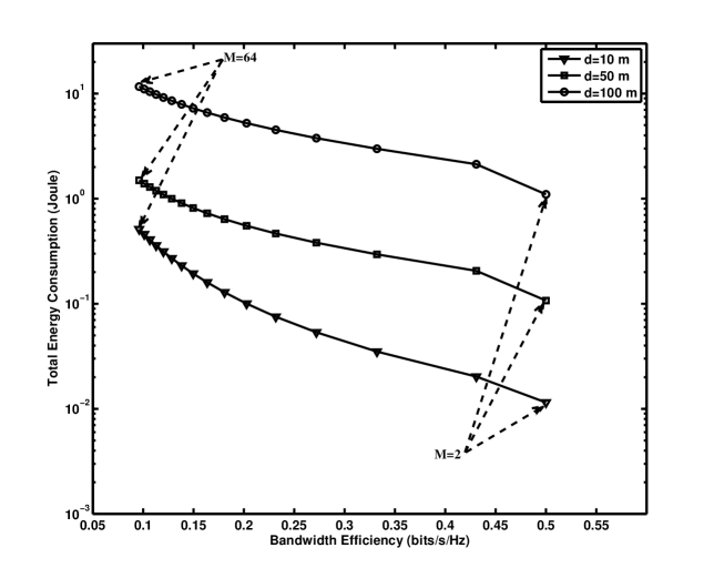
Figure 7: Total energy consumption of transmitting $N$ bits versus bandwidth efficiency for NC-MFSK, and for $P_{s}=10^{-3}$ and different values of $d$ and $M$.

For energy consumption analysis, we describe a conventional non-coherent receiver relating to the OOK scheme which is an energy detector receiver [33, 34]. This structure consists of a filter on the considered band, a square-law block, and an integrator followed by a decision block with an optimum threshold level (see [28, Fig. 7]). In addition, a low-noise amplifier is included in front-end. Using this non-coherent receiver, no oscillator is required for phase synchronization, and the receiver can turn on quickly. Note that when bit “0” is transmitted using OOK, the sensor node is silent, while at sink node, only band-pass noise is presented to the envelope detector. It can be shown in [35, pp. 490-504] that the BER conditioned upon $\gamma_{i}$ of a non-coherent OOK, denoted by $P_{b}(\gamma_{i})$, is upper bounded by $P_{b}(\gamma_{i})\leq\frac{1}{2}e^{-\frac{\gamma_{i}}{2}}$. Thus, the average BER of an OOK with non-coherent receiver, denoted by $P_{b}$, is upper bounded by

$$P_{b} = \int_{0}^{\infty}P_{b}(\gamma_{i})f_{\gamma}(\gamma_{i})d\gamma_{i}\leq\dfrac{1}{2\bar{\gamma}^{OK}}\int_{0}^{\infty}e^{-\gamma_{i}\left(\frac{1}{2}+\frac{1}{\bar{\gamma}^{OK}}\right)}d\gamma_{i}$$ (20)

$$= \dfrac{1}{\bar{\gamma}^{OK}+2},$$ (21)

where $\bar{\gamma}^{OK}=\frac{\Omega}{\mathcal{L}_{d}}\frac{\mathcal{E}^{OK}_{t}}{N_{0}}$ denotes the average received SNR. It should be noted that the average SER of OOK is the same as average BER. By approximating the above upper bound as an equality, the transmit energy consumption per each symbol for a given $P_{b}$ is obtained as $\mathcal{E}^{OK}_{t}\triangleq\mathcal{P}^{OK}_{t}T_{p}\approx\left(\frac{1}{P_{b}}-2\right)\frac{\mathcal{L}_{d}N_{0}}{\Omega}$, which is correspond to transmitting OOK bit “1”. Note that the energy consumption of transmitting $N$ bits during active mode (i.e., $\mathcal{P}^{OK}_{t}T^{OK}_{ac}$) is equivalent to the energy consumption of transmitting $L$ bits “1” in $(a_{1},...a_{N})$, where $L$ is a binomial random variable with parameters $(N,q)$. Assuming uncorrelated and equally likely binary data $a_{i}$, we have $q=\frac{1}{2}$. Hence, $\mathcal{P}^{OK}_{t}T^{OK}_{ac}=L\mathcal{E}^{OK}_{t}\approx L\left(\frac{1}{P_{b}}-2\right)\frac{\mathcal{L}_{d}N_{0}}{\Omega}$, where $L$ has the probability mass function $\textrm{Pr}\{L=\ell\}=\binom{N}{\ell}\left(\frac{1}{2}\right)^{N}$ with $\mathbb{E}[L]=\frac{N}{2}$.

The energy consumption of the sensor and sink circuitry during $T^{OK}_{ac}$ for a non-coherent OOK is computed as $(\mathcal{P}^{OK}_{ct}+\mathcal{P}^{OK}_{cr})T^{OK}_{ac}$. We denote the power consumptions of pulse generator, power amplifier and filter as $\mathcal{P}^{OK}_{PG}$, $\mathcal{P}^{OK}_{Amp}$ and $\mathcal{P}^{OK}_{Filt}$, respectively. Hence, the energy consumption of the sensor node circuitry during $T^{OK}_{ac}$ is represented as a function of random variable $L$ as $\mathcal{P}^{OK}_{ct}T^{OK}_{ac}\approx\mathcal{P}^{OK}_{PG}T^{OK}_{ac}+LT_{p}\left(\mathcal{P}^{OK}_{Filt}+\mathcal{P}^{OK}_{Amp}\right)$, where the factor $LT_{p}$ comes from the fact that filter and power amplifier are active only during transmitting $L$ bits “1”. We assume that $\mathcal{P}^{OK}_{Amp}=\alpha^{OK}\mathcal{P}^{OK}_{t}$, with $\alpha^{OK}=0.33$. In addition, the energy consumption of the sink circuitry with non-coherent detection OOK can be obtained as $\mathcal{P}^{OK}_{cr}T^{OK}_{ac}=\left(\mathcal{P}^{OK}_{LNA}+\mathcal{P}^{OK}_{ED}+\mathcal{P}^{OK}_{Filr}+\mathcal{P}^{OK}_{Int}+\mathcal{P}^{OK}_{ADC}\right)T^{OK}_{ac}$, where $\mathcal{P}^{OK}_{Int}$ is the power consumption of integrator unit. Also, with a similar argument as pass-band modulations, we assume that the circuit power consumption during $T^{OK}_{tr}$ is governed by the pulse generator block. As a result, the total energy consumption of a non-coherent OOK for transmitting $N$ bits is obtained as a function of random variable $L$ as follows:

$$\mathcal{E}^{OK}_{N}(L)=(1+\alpha^{OK})L\left(\dfrac{1}{P_{b}}-2\right)\dfrac{\mathcal{L}_{d}N_{0}}{\Omega}+(\mathcal{P}^{OK}_{cr}+\mathcal{P}^{OK}_{PG})\dfrac{2N}{B}+\dfrac{L}{B}\mathcal{P}^{OK}_{Filt}+2\mathcal{P}^{OK}_{PG}T^{OK}_{tr},$$ (22)

where we use $T^{OK}_{ac}=\frac{2N}{B}$. Using $\mathbb{E}[L]=\frac{N}{2}$, the average $\mathcal{E}^{OK}_{N}(L)$ is computed as

$$\mathcal{E}^{OK}_{N}\triangleq\mathbb{E}\left[\mathcal{E}^{OK}_{N}(L)\right]=(1+\alpha^{OK})\left(\dfrac{1}{P_{b}}-2\right)\dfrac{\mathcal{L}_{d}N_{0}}{\Omega}\dfrac{N}{2}+(\mathcal{P}^{OK}_{cr}+\mathcal{P}^{OK}_{PG})\dfrac{2N}{B}+\dfrac{N}{2B}\mathcal{P}^{OK}_{Filt}+2\mathcal{P}^{OK}_{PG}T^{OK}_{tr}.$$ (23)

M-ary PPM: In an M-PPM modulator each $b\triangleq\log_{2}M$ bits are encoded by transmitting a single pulse in one of $M=2^{b}$ possible time-shifts. This process is repeated every $T^{PP}_{s}$ seconds. An M-PPM signal constellation consists of a set of $M$ orthogonal pulses (in time) with equal energy. This is the time-domain dual to MFSK which uses a set of $M$ orthogonal carriers. Assuming Gaussian monocycle pulse with duration $T_{p}$ for pulse shaping, the channel bandwidth and data rate of M-PPM are determined as $B\approx\frac{1}{T_{p}}$ and $R^{PP}=\frac{b}{T^{PP}_{s}}$, respectively, where $T^{PP}_{s}=MT_{p}$ represents the time duration of a symbol. As a result, the bandwidth efficiency of an M-PPM scheme is obtained as $B^{PP}_{eff}\triangleq\frac{R^{PP}}{B}=\frac{\log_{2}M}{M}~{}\textrm{(bits/s/Hz)}$. For $M=2$, the bandwidth efficiency of M-PPM is the same as that of OOK with $50\%$ duty-cycle. For other values of $M$, the same $B^{PP}_{eff}$ is achieved through $\frac{T_{p}}{T^{OK}_{s}}=\frac{\log_{2}M}{M}$ with adjusting $T^{OK}_{s}$. In addition, similar to MFSK scheme, it can be seen that increasing constellation size $M$ leads to decrease in the bandwidth efficiency in M-PPM. To address the impact of increasing $M$ on energy efficiency, let derive the relationship between $M$ and the active mode duration $T^{PP}_{ac}$. Noting that during each symbol period $T^{PP}_{s}$, we have $b$ bits, it is concluded that $T^{PP}_{ac}=\frac{N}{b}T^{PP}_{s}=\frac{MN}{B\log_{2}M}$. With a similar argument as MFSK, increasing $M$ results in increasing in $T^{PP}_{ac}$, however $T^{PP}_{ac}$ is upper bounded by $T_{N}-T^{PP}_{tr}$. Thus, the maximum constellation size $M$, denoted by $M_{max}\triangleq 2^{b_{max}}$, for M-PPM is calculated by $\frac{2^{b_{max}}}{b_{max}}=\frac{B}{N}(T_{N}-T^{PP}_{tr})$.

As mentioned before, among current UWB receivers, the energy detection based non-coherent receiver is the simplest and most practical one to implement. The optimum non-coherent M-PPM receiver consists of a bank of $M$ matched filters, each followed by an envelop detector (see Fig. B.13 in [24]). At the sampling times $t=\ell T^{PP}_{s}$, a maximum-likelihood makes decision based on the largest filter output. It is shown that for non-coherent M-PPM, the SER conditioned upon $\gamma_{i}$ is obtained as follows [24, p. 969]

$$P_{s}(\gamma_{i})=\sum_{k=1}^{M-1}\dfrac{(-1)^{k+1}}{k+1}\binom{M-1}{k}e^{-\frac{k}{k+1}\gamma_{i}}.$$ (24)

The leading term of (24) provides an upper bound as $P_{s}(\gamma_{i})\leq\frac{M-1}{2}e^{-\frac{\gamma_{i}}{2}}$. For $M=2$, this upper bound becomes the exact expression. The average SER of a non-coherent M-PPM is then upper bounded by

$$P_{s} = \int_{0}^{\infty}P_{s}(\gamma_{i})f_{\gamma}(\gamma_{i})d\gamma_{i}\leq\dfrac{M-1}{2\bar{\gamma}^{PP}}\int_{0}^{\infty}e^{-\gamma_{i}\left(\frac{1}{2}+\frac{1}{\bar{\gamma}^{PP}}\right)}d\gamma_{i}$$ (25)

$$= \dfrac{M-1}{\bar{\gamma}^{PP}+2},$$ (26)

where $\bar{\gamma}^{PP}=\frac{\Omega}{\mathcal{L}_{d}}\frac{\mathcal{E}^{PP}_{t}}{N_{0}}$. For large $\bar{\gamma}^{PP}$, the upper bound (26) is the same as the upper bounded $P_{s}$ for MFSK. By approximating the upper bound (26) as an equality, the transmit energy consumption per each symbol for a given $P_{s}$ is obtained as $\mathcal{E}^{PP}_{t}\triangleq\mathcal{P}^{PP}_{t}T_{p}\approx\left(\frac{M-1}{P_{s}}-2\right)\frac{\mathcal{L}_{d}N_{0}}{\Omega}$. Noting that during active mode period $T_{ac}^{PP}$, we have $\frac{N}{b}$ monocycle pulses, the energy consumption of transmitting $N$ bits during active mode period is computed as $\mathcal{P}^{PP}_{t}T^{PP}_{ac}=\frac{N}{\log_{2}M}\mathcal{E}^{PP}_{t}\approx\left(\frac{M-1}{P_{s}}-2\right)\frac{\mathcal{L}_{d}N_{0}}{\Omega}\frac{N}{\log_{2}M}$. It can be seen that the energy consumption of transmitting $N$ bits during active mode period for M-PPM scheme is a monotonically increasing function of $M$.

The energy consumption of the sensor and the sink circuitry during active mode period $T^{PP}_{ac}$ for a non-coherent M-PPM is computed as $(\mathcal{P}^{PP}_{ct}+\mathcal{P}^{PP}_{cr})T^{PP}_{ac}$. The energy consumption of the sensor node circuitry during active mode duration is given by $\mathcal{P}^{PP}_{ct}T^{PP}_{ac}\approx\left(\mathcal{P}^{PP}_{PG}+\mathcal{P}^{PP}_{Filt}+\mathcal{P}^{PP}_{Amp}\right)\frac{N}{B\log_{2}M}$, where the factor $\frac{N}{B\log_{2}M}$ comes from the fact that transmitter circuitry is active only during $T_{p}$ in each period $T^{PP}_{s}$. We assume that $\mathcal{P}^{PP}_{Amp}=\alpha^{PP}\mathcal{P}^{PP}_{t}$, with $\alpha^{PP}=0.33$. With a similar argument as MFSK, the energy consumption of the sink circuitry with non-coherent detection M-PPM can be obtained as $\mathcal{P}^{PP}_{cr}T^{PP}_{ac}=\left(\mathcal{P}^{PP}_{LNA}+M\times\left(\mathcal{P}^{PP}_{ED}+\mathcal{P}^{PP}_{Filr}\right)+\mathcal{P}^{PP}_{ADC}\right)\frac{MN}{B\log_{2}M}$. As a result, the total energy consumption of a non-coherent M-PPM system for transmitting $N$ bits is obtained as

$$\mathcal{E}^{PP}_{N} = (1+\alpha^{PP})\left(\dfrac{M-1}{P_{s}}-2\right)\dfrac{\mathcal{L}_{d}N_{0}}{\Omega}\dfrac{N}{\log_{2}M}+(\mathcal{P}^{PP}_{ct}-\mathcal{P}^{PP}_{Amp})\dfrac{N}{B\log_{2}M}+$$ (28)

$$\mathcal{P}^{PP}_{cr}\dfrac{MN}{B\log_{2}M}+2\mathcal{P}^{PP}_{PG}T^{PP}_{tr}.$$

V Numerical Results

In this section, we present some numerical evaluations using realistic parameters in IEEE 802.15.4 standard and present state-of-the art technology to confirm the energy efficiency analysis of the pass-band and UWB modulation schemes mentioned in Sections III and IV. We also investigate the impact of constellation size $M$ and distance $d$ on the energy consumptions for M-ary modulation schemes. For numerical results, we assume that all modulation schemes operate in $f_{0}=$2.4 GHz Industrial Scientist and Medical (ISM) unlicensed band utilized in IEEE 802.15.14 for WSNs [16]. Also according to FCC 15.247 RSS-210 standard for United States/Canada, the maximum allowed antenna gain is 6 dBi [36]. In this work, we assume that $\mathcal{G}_{t}=\mathcal{G}_{r}=5$ dBi. Thus for $f_{0}=$2.4 GHz, $\mathcal{L}_{1}~{}\textrm{(dB)}\triangleq 10\log_{10}\left(\frac{(4\pi)^{2}}{\mathcal{G}_{t}\mathcal{G}_{r}\lambda^{2}}\right)\approx 30~{}\textrm{dB}$, where $\lambda\triangleq\frac{3\times 10^{8}}{f_{0}}$ in meter. As mentioned before, the channel bandwidth of UWB schemes is much wider than that of pass-band ones. Thus, due to the dependency of total energy consumption on bandwidth, comparing the energy efficiency of UWB schemes with that of pass-band ones would not meaningful. For this reason, we evaluate the energy efficiency of each category separately.

Pass-Band Modulation: We assume that in each period $T_{N}$, the sensed data frame size $N=1024$ bytes (or equivalently $N=8192$ bits) is generated for transmission for all the pass-band modulation schemes, where $T_{N}$ is assumed to be 1.4 second. The channel bandwidth is assumed to be $B=62.5$ KHz, according to IEEE 802.15.4 standard [16, p. 49]. The power consumption of LNA and IF amplifier are considered about 9 mw [37] and 3 mw [4, 5], respectively, which are assumed to be the same for all pass-band modulations. The power consumption of frequency synthesizer in MFSK is supposed to be 10 mw [7]. We use this value for the sinusoidal carrier generation in MQAM and OQPSK as well. We consider 7 mw power consumption for ADC and DAC [38]. In addition, we assume that the transceivers of the pass-band modulations are able to achieve values for $T_{tr}$ of about 5 $\mu s$ for MFSK and 20 $\mu s$ for MQAM and OQPSK [4, 38]. Table I shows the system parameters for simulation.

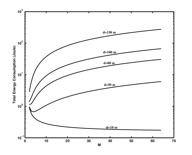
Figure 5: Total energy consumption $\mathcal{E}_{N}^{QA}$ vs. $M$ over Rayleigh fading channel model with path-loss for $P_{s}=10^{-3}$.

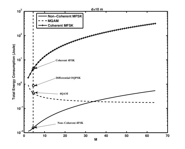
(a)

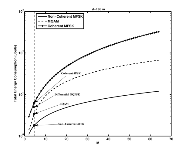
(b)

Figure 6: Total Energy consumption of transmitting $N$ bits vs. $M$ for MFSK, MQAM and differential OQPSK over Rayleigh fading channel model with path-loss and $P_{s}=10^{-3}$, a) $d=10$ m, and b) $d=100$ m.

It is concluded from $\frac{2^{b_{max}}}{\zeta b_{max}}=\frac{B}{N}(T_{N}-T^{FS}_{tr})$ that $M_{max}\approx 64$ (or equivalently $b_{max}\approx 6$) for NC-MFSK. Since, there is no constraint for $M$ in MQAM, we choose the range $2\leq M\leq 64$ for MQAM as well to be consistent with MFSK. Recalling from (4), the total energy consumption $\mathcal{E}_{N}^{FS}$ is a monotonically increasing function of $M$ for different values of $d$. While, the total energy consumption $\mathcal{E}_{N}^{QA}$ of MQAM in terms of $M$ displays different trend for each distance $d$ as depicted in Fig. 5. For instance, for $d=50$ m, the optimum value for $M$ that minimizes $\mathcal{E}_{N}^{QA}$ is 4 (equivalent to 4QAM scheme). Although the second term of (13) correspond to the circuit energy consumption of MQAM is a monotonically decreasing function of $M$, however for large values of $d$, the total energy consumption is governed by the $\mathcal{P}^{QA}_{t}T_{ac}^{QA}$ which results in $\mathcal{E}_{N}^{QA}$ to be a monotonically increasing function of $M$ when $d$ increases. Also, Fig. 6 compares the energy efficiency of the aforemention pass-band modulations versus $M$ for $P_{s}=10^{-3}$ and different values of $d$. It is revealed from Fig. 6-a that for $M<35$, NC-MFSK is more energy efficient than MQAM, OQPSK and coherent MFSK for $d=10$ m. In addition, NC-MFSK for small $M$ benefits from low complexity and cost in implementation over other schemes. Furthermore, as shown in Fig. 6-b, the total energy consumption of both MFSK and MQAM for large $d$ increase logarithmically when $M$ increases. Also, it can be seen that non-coherent 4FSK scheme consumes much less energy than the other schemes in short ranges of $d$.

Up to know, we have investigated the energy efficiency of pass-band modulation schemes under the assumption of Rayleigh fading channel model with path-loss, where there is no Line-Of-Sight (LOS) path between sensor and sink nodes. Of course, the Rayleigh fading channel is known to be a reasonable model for fading encountered in many wireless networks. However, it is also of interest to evaluate the energy efficiency of pass-band modulation schemes operating over the more general Rician model which includes a strong direct LOS path. This is because when WSNs work in short range environments, there is a high probability of LOS propagation [39]. For this purpose, let assume that the instantaneous channel coefficient correspond to symbol $i$ is $G_{i}=\frac{h_{i}}{\mathcal{L}_{d}}$, where $h_{i}$ is assumed to be Rician distributed with pdf $f_{h_{i}}(r)=\frac{r}{\sigma^{2}}e^{-\frac{r^{2}+A^{2}}{2\sigma^{2}}}I_{0}\left(\frac{rA}{\sigma^{2}}\right),~{}r\geq 0$, where $A$ denotes the peak amplitude of the dominant signal, $2\sigma^{2}\triangleq\Omega$ is the average power of non-LOS multipath components [40, p. 78]. For this model, $\mathbb{E}[|h_{i}|^{2}]=A^{2}+2\sigma^{2}=2\sigma^{2}(1+K)$, where $K(\textrm{dB})\triangleq 10\log\frac{A^{2}}{2\sigma^{2}}$ is the Rician factor. The value of $K$ is a measure of the severity of the fading. For instance, $K(\textrm{dB})\to-\infty$ implies Rayleigh fading and $K(\textrm{dB})\to\infty$ represents AWGN channel. It is seen from Table II that NC-MFSK with small order of $M$ has minimum total energy consumption compared to the other schemes in Rician fading channel model with path-loss. Although MQAM with large $M$ has less energy consumption than NC-MFSK with the same size $M$ for different values of $K$, however it is greater than that of NC-4FSK.

The above results make NC-MFSK attractive for using in WSNs, in particular for short to moderate range applications, since NC-MFSK already has the advantage of less complexity and cost in implementation than MQAM, differential OQPSK and coherent MFSK, and has less total energy consumption. In addition, since for typical energy-constrained WSNs, data rates are usually low, using small order of M-ary NC-FSK schemes are desirable. The sacrifice, however, is the bandwidth efficiency of NC-MFSK (when $M$ increases) which is a critical factor in band-limited WSNs. But in unlicensed bands where large bandwidth is available, NC-MFSK can be considered as a realistic option in WSNs. To have more insight into the behavior of this scheme, we plot the total energy consumption of NC-MFSK as a function of $B_{eff}^{FS}$ for different values of $M$ and $d$ in Fig. 7. In all cases, we observe that the minimum $\mathcal{E}_{N}^{FS}$ is achieved at low values of distance $d$ and for $M=2$, which corresponds to the maximum bandwidth efficiency $B_{eff}^{FS}=0.5$.

UWB Modulation: In WSNs with very short-range scenarios, it is desirable to use UWB schemes rather than pass-band ones, due to the inherent advantages of UWB wireless technology mentioned before. We assume that total number of transmission bits during $T_{N}$ for UWB modulations is $N=20000$, where $T_{N}$ is assumed to be 100 ms. As previously mentioned, the channel bandwidth of UWB modulation schemes is $B=500$ MHz for the ISM unlicensed band 2.4 GHz. In addition, since the main application of UWB systems is in very short-range scenarios, we assume $1\leq d\leq 10$ m which is a feasible range for UWB applications. The power consumption of LNA for an arbitrarily UWB receiver is considered 3.1 mw [41]. The power consumption of pulse generator is supposed to be 675 $\mu$w [42]. In addition, we assume that the transceivers of UWB schemes are able to achieve values for $T_{tr}$ of about 2 ns [43].

Fig. 8 plots the total energy consumption of M-PPM scheme versus $M$ for $P_{s}=10^{-3}$ and different distance $d$. The results show that the total energy consumption $\mathcal{E}_{N}^{PP}$ is still a monotonically increasing function of $M$ for different values of $d$. Also, Fig. 9 shows the graphs of total energy consumption of OOK and M-PPM for M=2, 4, 8 in terms of distance $d$ for $P_{s}=10^{-3}$. As shown in this figure, OOK performs better than M-PPM from the energy consumption points of view, for $1\leq d\leq 10$ m. As a result, OOK would be considered an appropriate option for using in very short-range WSN applications, since OOK already has the advantage of less complexity and cost in implementation than M-PPM, and has less total energy consumption.

VI Conclusion

In this paper, we have analyzed in-dept the energy efficiency of various modulation schemes to find the best scheme in a WSN over Rayleigh and Rician flat-fading channels with path-loss, using realistic models and parameters in IEEE 802.15.4 standard. Experimental results show that NC-MFSK is attractive for using in WSNs with short to moderate range applications, since NC-MFSK already has the advantage of less complexity and cost in implementation than MQAM and differential OQPSK, and has less total energy consumption. In addition, MFSK has faster start-up time than other pass-band schemes. Furthermore, since for typical energy-constrained WSNs, data transmission rates are usually low, using small order M-ary NC-FSK schemes are desirable. The sacrifice, however, is the bandwidth efficiency of NC-MFSK when $M$ increases. However, since most of WSN applications with band-pass modulation requires low to moderate bandwidth, a loss in the bandwidth efficiency can be tolerable, in particular for the unlicensed band applications where large bandwidth is available. In addition, one would use Minimum Shift Keying (MSK) scheme (as a special case of FSK), since it has some excellent spectral properties which make it an attractive alternative when other channel constraints require bandwidth efficiencies below 1.0 bit/s/Hz. In very short-range WSN applications, on the other hand, it is desirable to use UWB modulation schemes, rather than pass-band ones due to ultra-low power consumption and very low complexity in implementation. It was shown that OOK has the advantage of very simple complexity and lower cost in implementation than M-PPM, and has less total energy consumption.

Appendix A Energy Efficiency of Coherent MFSK

For the coherent MFSK, the precise frequency and carrier phase reference are available at the sink node. It is shown that the SER conditioned upon $\gamma_{i}$ of a coherent MFSK is obtained as $P_{s}(\gamma_{i})=1-\frac{1}{\sqrt{2\pi}}\int_{-\infty}^{\infty}e^{-\frac{u^{2}}{2}}\left[1-\textrm{erfc}\left(u+\sqrt{2\gamma_{i}}\right)\right]^{M-1}du\leq(M-1)Q(\sqrt{\gamma_{i}})\leq\frac{M-1}{2}e^{-\frac{\gamma_{i}}{2}}$, where we use $Q(x)\leq\frac{1}{2}e^{-\frac{x^{2}}{2}}$ [44, p. 383]. Thus, the average SER of a coherent MFSK is upper bounded by $P_{s}=\int_{0}^{\infty}P_{s}(\gamma_{i})f_{\gamma}(\gamma_{i})d\gamma_{i}\leq\frac{M-1}{2\bar{\gamma}}\int_{0}^{\infty}e^{-\gamma_{i}(\frac{1}{2}+\frac{1}{\bar{\gamma}^{FS}})}d\gamma_{i}=\frac{M-1}{\bar{\gamma}^{FS}+2}$, whit $\bar{\gamma}^{FS}=\frac{\Omega}{\mathcal{L}_{d}}\frac{\mathcal{E}^{FS}_{t}}{N_{0}}$. As a result, $\mathcal{E}^{FS}_{t}\triangleq\mathcal{P}^{FS}_{t}T^{FS}_{s}\leq\left[\frac{M-1}{P_{s}}-2\right]\frac{\mathcal{L}_{d}N_{0}}{\Omega}$. Approximating the above upper bound as an equality, the energy consumption of transmitting $N$ bits during active mode period is computed as $\mathcal{P}^{FS}_{t}T^{FS}_{ac}\approx\left[\frac{M-1}{P_{s}}-2\right]\frac{\mathcal{L}_{d}N_{0}}{\Omega}\frac{N}{\log_{2}M}$. The energy consumption of the sensor circuity for the coherent FSK is the same as that of the non-coherent case. For the power consumption of the sink circuity, however, we use the fact that each branch in coherent MFSK demodulator consists of carrier generator, mixer and band pass filter. Thus, $\mathcal{P}^{FS}_{cr}=\mathcal{P}^{FS}_{LNA}+M\times(\mathcal{P}^{FS}_{Sy}+\mathcal{P}^{FS}_{Mix}+\mathcal{P}^{FS}_{Filr})+\mathcal{P}^{FS}_{IFA}+\mathcal{P}^{FS}_{ADC}$. Using (2) with $\zeta=2$ for coherent MFSK, the total energy consumption of a coherent MFSK for transmitting $N$ bits during $T_{N}$ is obtained as $\mathcal{E}^{FS}_{N}=(1+\alpha^{FS})\left[\frac{M-1}{P_{s}}-2\right]\frac{\mathcal{L}_{d}N_{0}}{\Omega}\frac{N}{\log_{2}M}+(\mathcal{P}^{FS}_{c}-\mathcal{P}^{FS}_{Amp})\frac{MN}{2B\log_{2}M}+1.75\mathcal{P}^{FS}_{Sy}T^{FS}_{tr}$, under the constraint $M\leq M_{max}$.

Figure 8: Total energy consumption of transmitting $N$ bits versus $M$ for M-PPM over Rayleigh fading channel model with path-loss and $P_{s}=10^{-3}$.

Figure 9: Total energy consumption of transmitting $N$ bits versus $d$ for OOK and M-PPM with M=2,4,8, and for $P_{s}=10^{-3}$.

TABLE I: System Evaluation Parameters [11, 4]

	Pass-Band			UWB
$N=8192$ bits	$T_{N}=1.4$ sec	$\mathcal{P}_{DAC}=7$ mw	$N=20000$	$N_{0}=-180$ dB	$\mathcal{P}_{PG}=675$ $\mu$w
$B=62.5$ KHz	$N_{0}=-180$ dB	$\mathcal{P}_{ADC}=7$ mw	$B=500$ MHz	$T_{N}=100$ msec	$\mathcal{P}_{LNA}=3.1$ mw
$M_{l}=40$ dB	$\mathcal{P}_{Sy}=10$ mw	$\mathcal{P}_{Mix}=7$ mw	$M_{l}=40$ dB	$T_{tr}=2$ nsec	$\mathcal{P}_{ED}=3$ mw
$\mathcal{L}_{1}=30$ dB	$\mathcal{P}_{Filt}=2.5$ mw	$\mathcal{P}_{ED}=3$ mw	$\mathcal{L}_{1}=30$ dB	$\mathcal{P}_{Filt}=2.5$ mw	$\mathcal{P}_{ADC}=7$ mw
$\eta=3.5$	$\mathcal{P}_{Filr}=2.5$ mw	$\mathcal{P}_{IFA}=3$ mw	$\eta=3.5$	$\mathcal{P}_{Filr}=2.5$ mw	$\mathcal{P}_{Int}=3$ mw
$\Omega=1$	$\mathcal{P}_{LNA}=9$ mw

TABLE II: Total Energy Consumption (in Joule) of NC-MFSK, MQAM and OQPSK over Rician Fading Channel with Path-Loss

			$K=1$ dB			$K=10$ dB			$K=15$ dB
	$M$	OQPSK	NC-MFSK	MQAM	OQPSK	NC-MFSK	MQAM	OQPSK	NC-MFSK	MQAM
	4	1.1241	0.0173	0.5621	1.1241	0.0171	0.5620	1.1241	0.0171	0.5620
d=10 m	16		0.0769	0.2819		0.0765	0.2810		0.0765	0.2810
	64		0.6558	0.1924		0.6545	0.1874		0.6545	0.1874
	4	1.2236	0.5835	0.8873	1.1445	0.0194	0.5652	1.1310	0.0175	0.5627
d=100 m	16		1.4920	3.2049		0.0785	0.2989		0.0767	0.2843
	64		4.6199	16.1010		0.6570	0.2615		0.6547	0.2002

References

- [1] J. Abouei, K. N. Plataniotis, and S. Pasupathy, “Green modulation in dense wireless sensor networks,” Submitted to IEEE International Conference on Acoustics, Speech and Signal Processing (ICASSP’10), Sept. 2009.
- [2] W. Ye, J. Heidemann, and D. Estrin, “An energy-efficient MAC protocol for wireless sensor networks,” in Proc. of INFOCOM. New York, June 2002, pp. 1567–1576.
- [3] H. Kwon, T. H. Kim, S. Choi, and B. G. Lee, “A cross-layer strategy for energy-efficient reliable delivery in wireless sensor networks,” IEEE Trans. on Wireless Commun., vol. 5, no. 12, pp. 3689–3699, Dec. 2006.
- [4] S. Cui, A. J. Goldsmith, and A. Bahai, “Energy-constrained modulation optimization,” IEEE Trans. on Wireless Commun., vol. 4, no. 5, pp. 2349–2360, Sept. 2005.
- [5] Q. Tang, L. Yang, G. B. Giannakis, and T. Qin, “Battery power efficiency of PPM and FSK in wireless sensor networks,” IEEE Trans. on Wireless Commun., vol. 6, no. 4, pp. 1308–1319, April 2007.
- [6] F. Qu, D. Duan, L. Yang, and A. Swami, “Signaling with imperfect channel state information: A battery power efficiency comparison,” IEEE Trans. on Signal Processing, vol. 56, no. 9, pp. 4486–4495, Sep. 2008.
- [7] A. Y. Wang, S.-H. Cho, C. G. Sodini, and A. P. Chandrakasan, “Energy efficient modulation and MAC for asymmetric RF microsensor systems,” in Proc. of ISLPED’01. Huntington Beach, Calif, USA, Aug. 2001, pp. 106–111.
- [8] F. Qu, L. Yang, and A. Swami, “Battery power efficiency of PPM and OOK in wireless sensor networks,” in Proc. of IEEE International Conference on Acoustics, Speech and Signal Processing (ICASSP’07), 2007, pp. 525–528.
- [9] M. C. Gursoy, “On the energy efficiency of orthogonal signaling,” in Proc. of IEEE International Symposium on Information Theory (ISIT’08). Toronto, Canada, July 2008, pp. 599–603.
- [10] C. C. Enz, N. Scolari, and U. Yodprasit, “Ultra low-power radio design for wireless sensor networks,” in Proc. of IEEE Int. Workshop on Radio-Frequency Integration Technology. Dec. 2005, pp. 1–17, (Invited Paper).
- [11] H. Karl and A. Willig, Protocols and Architectures for Wireless Sensor Networks, John Wiley and Sons Inc., first edition, 2005.
- [12] X. Liang, W. Li, and T. A. Gulliver, “Energy efficient modulation design for wireless sensor networks,” in Proc. IEEE Pacific Rim Conf. on Commun., Computers and Signal Processing (PACRIM’07), Aug. 2007, pp. 98–101.
- [13] H. Karvonen, Z. Shelby, and C. Pomalaza-Raez, “Coding for energy efficient wireless embedded networks,” in Proc. of IEEE International Workshop on Wireless Ad-Hoc Networks, June 2004, pp. 300–304.
- [14] B. Shen and A. Abedi, “Error correction in heterogeneous wireless sensor networks,” in Proc. of 24th IEEE Biennial Symposium on Communication. Kingston, Canada, June 2008.
- [15] J. E. Garz s, C. B. Calz n, and A. G. Armada, “An energy-efficient adaptive modulation suitable for wireless sensor networks with SER and throughput constraints,” EURASIP Journal on Wireless Communications and Networking, vol. 2007, no. 1, Jan. 2007.
- [16] IEEE Standards, “Part 15.4: Wireless Medium Access control (MAC) and Physical Layer (PHY) Specifications for Low-Rate Wireless Personal Area Networks (WPANs),” in IEEE 802.15.4 Standards, Sept. 2006.
- [17] C. M. Cordeiro and D. P. Agrawal, Ad Hoc and Sensor Networks: Theory and Applications, World Scientific Publishing, 2006.
- [18] S. Mingoo, S. Hanson, D. Sylvester, and D. Blaauw, “Analysis and optimization of sleep modes in subthreshold circuit design,” in Proc. 44th ACM/IEEE Design Automation Conference, June 2007, pp. 694–699.
- [19] H. T. Friis, “A note on a simple transnission formula,” in Proc. IRE, 1946, vol. 34, pp. 245–256.
- [20] S. Tanchotikul, P. Supanakoon, S. Promwong, and J. Takada, “Statistical model RMS delay spread in UWB ground reflection channel based on peak power loss,” in Proc. of ISCIT’06, 2006, pp. 619–622.
- [21] L. Barclay, Propagation of Radiowaves, The Institution of Electrical Engineers, London, second edition, 2003.
- [22] J. G. Proakis, Digital Communications, New York: McGraw-Hill, forth edition, 2001.
- [23] R. Min and A. Chadrakasan, “A framework for energy-scalable communication in high-density wireless networks,” in Proc. of International Syposium on Low Power Electronics Design, 2002.
- [24] F. Xiong, Digital Modulation Techniques, Artech House, Inc., second edition, 2006.
- [25] R. E. Ziemer and R. L. Peterson, Digital Communications and Spread Spectrum Systems, New York: Macmillman, 1985.
- [26] R. A. Khalona, “Optimum Reed-Solomon codes for M-ary FSK modulation with hard decision decoding in Rician-fading channels,” IEEE Trans. on Commun., vol. 44, no. 4, pp. 409–412, April 1996.
- [27] M. K. Simon and M.-S. Alouini, Digital Communication over Fading Channels, New York: Wiley Interscience, second edition, 2005.
- [28] J. Abouei, K. N. Plataniotis, and S. Pasupathy, “Green modulation in proactive wireless sensor networks,” Technical report, University of Toronto, ECE Dept., Sept. 2009, available at http://www.dsp.utoronto.ca/ abouei/.
- [29] M. K. Simon, “Multiple-bit differential detection of offset QPSK,” IEEE Trans. on Commun., vol. 51, pp. 1004–1011, June 2003.
- [30] J. I. Marcum, “Table of Q Functions, U.S. Air Force Project RAND Res. Memo. M-339,” Jan. 1950, Rand Corp., Santa Monica, CA.
- [31] I. Oppermann, M. Hamalainen, and J. Iinatti, UWB Theory and Applications, John Wiley and Sons, 2004.
- [32] K. Fazel and S. Kaiser, Multi-Carrier and Spread Spectrum Systems, John Wiley and Sons Inc., first edition, 2003.
- [33] H. Urkowitz, “Energy detection of unknown deterministic signals,” Proc. of IEEE, vol. 55, no. 4, pp. 523–531, April 1967.
- [34] S. Paquelet and L. M. Aubert, “An energy adaptive demodulation for high data rates with impulse radio,” in Proc. of IEEE Radio and Wireless Conference, Sept. 2004, pp. 323–326.
- [35] L. W. Couch, Digital and Analog Communication Systems, Prentice-Hall, sixth edition, 2001.
- [36] “Range extension for IEEE 802.15.4 and ZigBee applications,” FreeScale Semiconductor, Application Note, Feb. 2007.
- [37] A. Bevilacqua and A. M. Niknejad, “An ultrawideband CMOS low-noise amplifier for 3.1-10.6 GHz wireless receivers,” IEEE Journal of Solid-State Circuits, vol. 39, no. 12, pp. 2259–2268, Dec. 2004.
- [38] G. Bravos and A. Kanatas, “Energy consumption and trade-offs on wireless sensor networks,” in Proc. IEEE PIMRC’05, Sept. 2005.
- [39] S. Wyne, A. P. Singh, F. Tufvesson, and A. F. Molisch, “A statistical model for indoor office wireless sensor channels,” IEEE Trans. on Wireless Commun., vol. 8, no. 8, pp. 4154–4164, August 2009.
- [40] A. Goldsmith, Wireless Communications, Cambridge University Press, first edition, 2005.
- [41] Y.-C. Lee and J.-H. Tarang, “A low power CMOS LNA for ultra-wideband wireless receivers,” IEICE Electronics Express, vol. 4, no. 9, pp. 294–299, May 2007.
- [42] X. Zhang, S. Ghosh, and M. Bayoumi, “A low power CMOS UWB pulse generator,” in Proc. of 48th IEEE International Symposium on Circuits and Systems (ISCAS’05), Aug. 2005, vol. 2, pp. 1410–1413.
- [43] V. De Heyn, G. V. der Plas, J. Ryckaert, and J. Craninckx, “A fast start-up 3 GHz-10 GHz digitally controlled oscillator for UWB impulse radio in 90 nm CMOS,” in Proc. of 33rd European Solid State Circuits Conference (ESSCIRC’07), Sept. 2007, pp. 484–487.
- [44] D. R. Smith, Digital Transmission Systems, Kluwer Academic Publishers, third edition, 2004.
(a)
(b)