STEP-FREQUENCY RADAR WITH COMPRESSIVE SAMPLING (SFR-CS)

Abstract

This paper proposes a novel radar system, namely step-frequency with compressive sampling (SFR-CS), that achieves high target range and speed resolution using significantly smaller bandwidth than traditional step-frequency radar. This bandwidth reduction is accomplished by employing compressive sampling ideas and exploiting the sparseness of targets in the range-speed space.

Index Terms— step frequency radar, compressive sampling, narrowband radar

1 Introduction

Since the advent of radar systems much of the efforts have been devoted to increasing radar range resolution. The relationship between range resolution and signal bandwidth is given by $\Delta R=\frac{c}{2B}$ where $\Delta R$ denotes range resolution, $c$ is the speed of light and $B$ is the bandwidth of the signal being used. Hence, wideband radar systems can achieve higher resolution than their narrow-band counterparts. However, wideband signals correspond to short pulses that experience low signal-to-noise ratio (SNR) at the receiver. Further, they require high speed A/Ds, and fast processors [1]. Step-frequency radar (SFR) achieves high range resolution without sharing the disadvantages of wideband systems. SFR transmits several narrowband pulses at different frequencies. The frequency remains constant during each pulse but increases in steps of $\Delta f$ between consecutive pulses. Thus, while its instantaneous bandwidth is narrow, the SFR system has a large effective bandwidth. Conventional step-frequency radars obtain one sample from each received pulse and then apply an inverse discrete Fourier transform (IDFT) on the phase detector output sequence for detection. Since the IDFT resolution increases with the number of transmitted pulses, SFR requires a large number of transmit pulses, or equivalently, large effective bandwidth.

In this paper, we propose a step-frequency radar with compressed sampling, that assuming the existence of a small number of targets exploits the sparseness of targets in the range-speed space. The application of compressive sampling to narrow-band radar systems was recently investigated in [2]-[6]. A CS-based data acquisition and imaging method was proposed in [7] for stepped-frequency continuous-wave ground penetrating radars (SFCW-GPRs). In [8], CS-based step frequency was applied on through-the-wall radar imaging (TWRI). In [7],[8] the authors have assumed stationary targets and have shown that the the CS approach can provide a high-quality radar image using much fewer data samples than conventional methods. Unlike [7],[8], the work in this paper explores joint target range and speed estimation based on compressive sampling, and proposes a radar system with reduced effective bandwidth as compared to traditional SFR systems.

2 Background information

Compressive sampling (CS) [9]-[11] has received considerable attention recently, and has been applied successfully in diverse fields, e.g., image processing [12] and wireless communications [13][14]. The theory of CS states that a $K$-sparse signal $\mathbf{x}$ of length $M$ can be recovered exactly with high probability from $\mathcal{O}(K\log M)$ measurements via $\ell_{1}$-optimization. Let $\mathbf{\Psi}$ denote the basis matrix that spans this sparse space, and let $\mathbf{\Phi}$ denote a measurement matrix. The convex optimization problem arising in CS is formulated as follows: $\min\|\mathbf{s}\|_{1},\ \ s.t.\ {\bf y}=\mathbf{\Phi}{\bf x}=\mathbf{\Phi}\mathbf{\Psi}{\bf s}=\mathbf{\Theta}\mathbf{s}$ where ${\mathbf{s}}$ is a sparse vector with $K$ principal elements and the remaining elements can be ignored; $\mathbf{\Phi}$ is an $N\times M$ matrix with $N\ll M$, that is incoherent with $\mathbf{\Psi}$. It has been shown that two properties govern the design of a stable measurement matrix: restricted isometry property and incoherence property [11]. A $K$-sparse signal $\mathbf{x}$ of length-$M$ can be recovered from $N<M$ samples provided $N\geq K$ and $\mathbf{\Theta}$ satisfies $1-\epsilon\leq\frac{\|\mathbf{\Theta}\mathbf{v}\|_{2}}{\|\mathbf{v}\|_{2}}\leq 1+\epsilon$ where $\mathbf{v}$ is an arbitrary $K$-sparse signal and $\epsilon>0$. This property is referred to as Restricted Isometry Property (RIP). The incoherence property suggests that the rows $\{\phi_{i}\}$ of ${\mathbf{\Phi}}$ should be incoherent with the columns $\{\psi_{j}\}$ of $\mathbf{\Psi}$.

Let us consider an SFR system that transmits $N$ pulses and waits for echoes of all pulses to return before it starts any processing. The frequency of $k^{th}$ pulse equals

$$f_{k}=f_{0}+k\Delta f$$ (1)

where $f_{0}$ is the starting frequency and $k\in\{0,1,2,...,N-1\}$. The $k^{th}$ transmit pulse is of the form $rect(t)\ e^{-i2\pi f_{k}t}$.

The signal reflected by a target at distance $R$ moving with speed $v$ is

$$r(t)=rect(t-\frac{2R}{c})\ e^{-i2\pi f_{k}(t-\frac{2}{c}(R+vkT))}$$ (2)

where $c$ is the speed of light, $T$ is the pulse repetition interval (PRI). Here we assume that $v$ is small enough to be considered constant within the pulse interval.

As we assume each pulse to be narrowband, we can ignore the delay of $\frac{2R}{c}$ in the signal envelope, and just consider the phase shift for extracting the information on targets. Therefore we have

$$r(t)=rect(t)\ e^{-i2\pi f_{k}(t-\frac{2}{c}(R+vkT))}$$ (3)

and the output of phase detector is of the form

$$y_{k}=e^{i2\pi(f_{0}+k\Delta f)\frac{2}{c}(R+vkT)}$$ (4)

The exponent of (4) can be written as

$$\gamma_{k}=\frac{4\pi}{c}f_{0}R\ +\ 2\pi\frac{2\Delta fR}{c}k\ +\ 2\pi\frac{2f_{0}vT}{c}k\ +\ 2\pi\frac{2k\Delta fvT}{c}k$$ (5)

The first term in (5) represents a constant phase shift due to the starting frequency, while the second term represents the phase shift due to frequency offset of the $k-$th pulse. The maximum unambiguous range and range resolution for step-frequency radar are given by $R_{u}=\frac{c}{2\Delta f}$ and $\Delta R=\frac{c}{2N\Delta f}$ respectively. Here $N\Delta f$ is the total effective bandwidth of the signal over $N$ pulses. Targets which are at distance $\tilde{R}>R_{u}$ will be seen by the system to be at distance $\tilde{R}-R_{u}$.

The third term of (5) gives the Doppler frequency shift experienced by the signal due to the target speed $v$. The fourth term of (5) represents the frequency spread due to target speed. This has the effect of spreading the energy of the main lobe at the target position.

3 The proposed approach

Let us take the transmitter and receiver to be co-located and employ $N$ pulses for estimating the range and speed of targets. Let us discretize the range space as $[R_{1},\ldots,R_{M}]$, and the speed space as $[v_{1},\ldots,v_{L}]$. The whole target scene can be described using $M\times L$ grid points in the range-speed plane. The range and speed spaces discretization steps are $\Delta R=\frac{R_{M}-R_{1}}{M-1}$ and $\Delta v=\frac{v_{L}-v_{1}}{L-1}$, respectively. We assume that the targets can be present only on the grid points. By representing the target scene as a matrix $\mathbf{S}$ of size $M\times L$, equation (4) becomes

$$y_{k}=\sum_{m=1}^{M}\sum_{l=1}^{L}e^{i2\pi f_{k}\frac{2}{c}(R_{m}+v_{l}kT)}\cdot S(m,l)+w_{k}$$ (6)

where

$$S(m,l)=\begin{cases}\alpha&\text{reflectivity of target present at $(R_{m},v_{l})$ }\\ 0&\text{if target is absent at $((m-1)L+l)^{th}$ grid point}\end{cases}$$ (7)

and $w_{k}$ represents zero-mean white noise.

Putting the outputs of phase of the phase detector, i.e., $y_{k},k=1,...,N$ in vector ${\bf y}$, we get

$${\bf y}={\mathbf{\Psi}}{\bf s}+{\bf w}$$ (8)

where $\mathbf{s}=[s_{1},s_{2},...,s_{ML}]^{T}$, ${\bf w}$ represents white zero-mean measurement noise, and the elements of matrix ${\mathbf{\Psi}}$ equal

$$\psi(k,(m-1)L+l)=e^{i2\pi(f_{0}+k\Delta f)\frac{2}{c}(R_{m}+v_{l}kT)}$$ (9)

for $k=1,...,N$, $m=1,...,M,\ l=1,...,L$. We can think of the basis matrix $\bf\Psi$ as being a stack of column vectors $\{\mathbf{\Psi}_{i}\}_{i=0}^{ML-1}$, i.e.,

$$\mathbf{\Psi}=(\ \mathbf{\Psi}_{0}\ |\ \mathbf{\Psi}_{1}\ |...|\ \mathbf{\Psi}_{ML-1}\ )$$ (10)

where each $\mathbf{\Psi}_{i}$ is of size $N\times 1$ containing the phase detector outputs for all $N$ pulses corresponding to the phase shift due to a target located at the $i^{th}$ grid point. Thus, ${\mathbf{\Psi}}$ accounts for the phase shift of all possible combinations of range and speed. Taking the measurement matrix ${\mathbf{\Phi}}$ to be an $N\times N$ identity matrix yields ${\mathbf{\Theta}}={\mathbf{\Psi}}$.

Based on (8) we can recover $\mathbf{s}$ by applying the Dantzig selector to the convex problem ([15])

$$\hat{{\bf s}}=\min\|{\bf s}\|_{1}\ \ \ s.t.\ \|{\mathbf{\Theta}}^{H}({\bf r}-\mathbf{\Theta}{\bf s})\|_{\infty}<\mu.$$ (11)

According to [15], the sparse vector ${\bf s}$ can be recovered with very high probability if $\mu=(1+t^{-1})\sqrt{2\log N\tilde{\sigma}^{2}}\sigma_{max}$, where $t$ is a positive scalar, $\sigma_{max}$ is the maximum norm of columns in the sensing matrix $\Theta$ and $\tilde{\sigma^{2}}$ is the variance of the noise in (6). A lower bound is readily available, i.e., $\mu>\sqrt{2\log N\tilde{\sigma}^{2}}\sigma_{max}$. Also, $\mu$ should not be too large because in that case the trivial solution ${\bf s}={\bf 0}$ is obtained. Thus, we may set $\mu<\|\Theta^{H}{\bf r}\|_{\infty}$.

In conventional SFR systems, the IDFT algorithm requires the columns of the transform matrix to be orthogonal. The range resolution in space depends on the frequency resolution in the Fourier domain. Therefore, these systems require $N=M$ pulses in order to have a range resolution of $\frac{R_{u}}{M}$. For the proposed approach we can use $N<M$ pulses and still achieve a range resolution of $\frac{R_{u}}{M}$.

For moving targets, the conventional IDFT method for estimating range and speed observes a shift in the target positions (due to speed) and a spreading effect around the shifted position (due to the fourth term in equation (5)). These effects degrade the receiver performance causing erroneous range estimation and sometimes missing the target completely. In the proposed approach, since ${\mathbf{\Psi}}$ has columns corresponding to all the possible range-speed combinations, the estimated results are comparatively more accurate.

4 Simulation Results

Stationary targets - Our simulations use the following parameter values: $f_{0}=1$MHz, $\Delta f=10$KHz, number of grid points $M=100$. These values of $\Delta f$ give $R_{u}=15\ Km$, and $\Delta R=150\ m$. We assume that the stationary point targets are present on the grid points. $100$ iterations of sparse target vectors are generated and the estimation accuracy is computed as the ratio of number of iterations for which the target ranges are correctly estimated to the total number of iterations.

The basis matrix $\bf\Psi$ of size $N\times M$ is generated according to equation (9). The measurement matrix $\bf\Phi$ is an identity matrix $\mathbf{I}$ of size $N\times N$. The optimization algorithm used to solve equation (11) was obtained from [16].

The number of pulses, $N$, controls the column correlation of the measurement matrix for a given value of $M$ (number of grid points). Lowering the correlation between adjacent columns of $\mathbf{\Psi}$ increases the isolation among the columns, which results in better range estimation.

For the measurement matrix generated by using equation (9), the adjacent column cross-correlation equals

$$R_{\phi}=\frac{1}{N}\ \frac{1-e^{-i2\pi\frac{N}{M}}}{1-e^{-i2\pi\frac{1}{M}}}$$ (12)

Figure 1 shows the effect of changing the column correlation on the estimation accuracy of the CS sensing matrix when the unambiguous range is divided into $100$ grid points. Figure 2 shows the accuracy of the CS detector in the presence of noise at different SNR values for the case in which only $5$ targets are within the detectable range. The noise signal added at the received signal was Gaussian zero-mean with variance $\sigma_{N}^{2}$, where the variance $\sigma_{N}^{2}$ changes with SNR. Figure 3 compares the performance of the CS detector with the conventional IDFT detector for $N=70$ for a target scene containing $5$ stationary targets. As it can be seen, the CS detector performs better than the IDFT detector for all SNRs. Figures 2 and 3 show that we can use $N<M$ pulses to obtain $\Delta R=\frac{1}{M}$, provided that $N=O(K\log N)$. This proves that we can use lower bandwidths in CS compared to conventional techniques of IDFT and accurately estimate the target parameters, when the targets are sparsely present in the range-speed space.

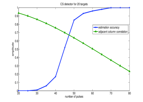
Fig. 1: Effect of changing column correlation on estimation accuracy for $100$ grid points for stationary target scenario

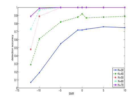
Fig. 2: Accuracy of CS detector at different SNR values for $5$ stationary targets

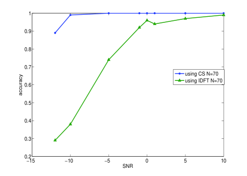
Fig. 3: Accuracy comparison between CS and IDFT detectors for $N=70$ and $5$ stationary targets.

Moving targets - The number of grid points in the range domain is taken to be $M=40$. $L=6$ grid points were used for discretizing the speed axis. The carrier frequency is $f=10^{8}Hz$ and the step frequency $\Delta f=10^{5}Hz$. The ranges and speeds of $4$ targets are generated randomly in each of $100$ Monte Carlo runs. Out of $4$ targets, two targets are placed on adjacent grid points on the range-speed space in each run. The accuracy of the detector is computed as the ratio of the number of runs for which all target ranges and speeds have been estimate accurately to the total number of runs. In Fig. 4, we show the detection accuracy of CS and IDFT methods for different values of SNR. For moving targets, the IDFT method requires speed compensation before performing IDFT. Since the target speed is unknown, we compensate the received signal with all possible speed and choose the one with the highest and sharpest IDFT output. As it can be seen, the proposed CS significantly improves the detection accuracy as compared to the IDFT method. The advantage of the CS approach is more obvious at low SNR. Figure 5 compares the detection accuracy of the CS and the IDFT methods for different number of pulses for $SNR=15dB$. We can easily see that the proposed method requires much fewer pulses than the IDFT method to achieve the same accuracy level. For example, the CS approach requires $130$ pulses to achieve detection accuracy of $0.95$, while the IDFT method needs about $190$ pulses in this particular case considered in our simulations.

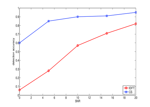
Fig. 4: Accuracy comparison between CS and IDFT detectors for different values of SNR for $N=100$ pulses (moving targets).

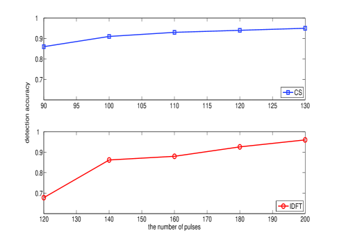
Fig. 5: Accuracy comparison between CS and IDFT detectors for different number of pulses at $SNR=15$dB (moving targets).

One trade-off that is not apparent from the simulations is computation time. Convex optimization techniques have much higher computation cost as compared to the IDFT. The basis pursuit (BP) algorithm used in our simulations has a computation complexity of $O((ML)^{3})$. Thus the processing speed of the receiver system may put a limit on the number of grid points $ML$ that can be used and the range resolution $\Delta R$. However there have been other algorithms like Orthogonal Matching Pursuit (OMP) which have computation complexities of $O(NKML)$. A decoupled range-speed estimation approach along the lines of [17] could also be employed here to reduce complexity.

5 Conclusion

We have proposed a CS-based SFR system for joint range-speed estimation. It has been shown by our simulation results that the proposed CS approach can achieve high resolution while employing lower effective bandwidth than traditional SFR systems. Unlike the IDFT method, the proposed approach does not suffer from range shift and range spreading around the shift positions caused by the movement of targets.

Acknowledgment

The authors wish to thank Dr. R. Madan of The Office of Naval Research for his insightful suggestions during the course of this work.

References

- [1] Gill,G.S. ”High-Resolution Step Frequency Radar” Ultra-Wideband Radar Technology, CRC Press.
- [2] R. Baraniuk and P. Steeghs, “Compressive Radar Imaging,” Proc. Radar Conference, pp. 128 - 133, April, 2007.
- [3] A. C. Gurbuz, J. H. McClellan and W.R. Scott, “Compressive sensing for GPR imaging,” Proc. 41th Asilomar Conf. Signals, Syst. Comput, pp. 2223-2227, Pacific Grove, CA, Nov. 2007.
- [4] M. Herman and T. Strohmer, “Compressed rensing radar,” in Proc. IEEE Int’l Conf. Acoust. Speech Signal Process, Las Vegas, NV, pp. 2617 - 2620, Mar. - Apr. 2008.
- [5] Y. Yu, A. P. Petropulu and H. V. Poor, “Compressive sensing for MIMO Radar,” in Proc. IEEE International Conference on Acoustics Speech and Signal Processing, pp. 3017 - 3020, Taipei, Taiwan, April, 2009.
- [6] Y. Yu, A. Petropulu and H.V. Poor, MIMO Radar Using Compressive Sampling, IEEE Journal on Selected Topics in Signal Proc., to appear in February 2010.
- [7] A.C. Gurbuz, J.H. McClellan and W.R. Scott, “A compressive sensing data acquisition and imaging method for stepped frequency GPRs,” : IEEE Transactions on Signal Processing, vol. 57, pp. 2640-2650, July 2009.
- [8] Y-S. Yoon and M. G. Amin, “Imaging of behind the wall targets using wideband beamforming with compressive sensing,” in Proc. IEEE Workshop on Statistical Signal Processing (SSP2009), Cardiff, Wales (UK), pp. 93-96, August 2009.
- [9] D. V. Donoho, “Compressed sensing,” IEEE Trans. Inf. Theory, vol. 52, pp. 1289-1306, no. 4, April 2006.
- [10] E. J. Candes, “Compressive sampling,” Proc. of Int. Congress of Math, Madrid, Spain, 2006.
- [11] Richard Baranuik ”Compressive Sensing”, Lecture Notes, IEEE Signal Processing Magazine, July 2007.
- [12] J. Romberg, “Imaging via compressive sampling [Introduction to compressive sampling and recovery via convex programming],” IEEE Signal Process. Mag., vol. 25, no. 2, pp. 14 - 20, Mar. 2008.
- [13] W. Bajwa, J. Haupt, A. Sayeed and R. Nowak, “Compressive wireless sensing,” in Proc. IEEE Inform. Process. in Sensor Networks, Nashville, TN, pp. 134 - 142, Apr. 2006.
- [14] J. L.Paredes, G. R. Arce, Z. Wang, “Ultra-wideband compressed sensing: Channel estimation,” IEEE Journal of Selected Topics in Signal Processing, vol.1, pp. 383 - 395, Oct. 2007.
- [15] E. Candes and T. Tao, “The Dantzig selector: Statistical estimation when is much larger than ,” Ann. Statist., vol. 35, pp. 2313-2351, 2007.
- [16] M.Grant, S.Boyd, Y.Ye ”cvx: Matlab Software for Disciplined convex programming” [Online] http://www.stanford.edu/ boyd/cvx/
- [17] Y. Yu, A.P. Petropulu and H.V. Poor, “Reduced complexity angle-doppler-range estimation for MIMO radar that employs compressive sensing,” Proc. 43nd Asilomar Conf. Signals, Syst. Comput, Pacific Grove, CA, Nov. 2009.