Pearson Walk with Shrinking Steps in Two Dimensions

Abstract

We study the shrinking Pearson random walk in two dimensions and greater, in which the direction of the $N^{\rm th}$ step is random and its length equals $\lambda^{N-1}$, with $\lambda<1$. As $\lambda$ increases past a critical value $\lambda_{c}$, the endpoint distribution in two dimensions, $P(\mathbf{r})$, changes from having a global maximum away from the origin to being peaked at the origin. The probability distribution for a single coordinate, $P(x)$, undergoes a similar transition, but exhibits multiple maxima on a fine length scale for $\lambda$ close to $\lambda_{c}$. We numerically determine $P(\mathbf{r})$ and $P(x)$ by applying a known algorithm that accurately inverts the exact Bessel function product form of the Fourier transform for the probability distributions.

I Introduction

In this work, we investigate the probability distribution of the shrinking Pearson random walk in two and greater dimensions, in which the length of the $N^{\rm th}$ step equals $\lambda^{N-1}$, with $\lambda<1$. If a walk is at $\mathbf{r}_{N}$ after the $N^{\rm th}$ step, then $\mathbf{r}_{N+1}$ is uniformly distributed on the surface of a sphere of radius $\lambda^{N}$ centered about $\mathbf{r}_{N}$ (Fig. 1). We assume that the walk begins at the origin, and the length of the first step is $\lambda^{0}=1$. The random direction for each step corresponds to the classic Pearson walk pearson ; W94 , whose solution is well known when the length of each step is fixed. In this case, the central limit theorem guarantees that the asymptotic probability distribution of endpoints approaches a Gaussian function.

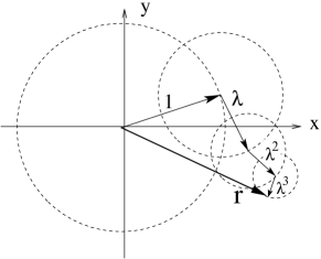
Figure 1: Illustration of the first four steps of a shrinking Pearson walk in two dimensions, leading to a displacement $\mathbf{r}$.

In one dimension, the random walk with exponentially shrinking step lengths exhibits a variety of beautiful properties W ; E . For $\lambda<\frac{1}{2}$, the support of the endpoint distribution after $N$ steps, $P_{N}(x)$, is a Cantor set, while for $\lambda>\frac{1}{2}$ the support is the connected interval $[-\frac{1}{1-\lambda},\frac{1}{1-\lambda}]$. More interestingly, for $\frac{1}{2}<\lambda<1$ and for $N\to\infty$, $P_{N}(x)$ is continuous for almost all values of $\lambda$, but is fractal on a complementary and infinite discrete set of $\lambda$ values W ; E ; G ; Kac . A particularly striking special case is $\lambda=g\equiv\frac{1}{2}(\sqrt{5}-1)=0.618\ldots$ (the inverse of the golden ratio), where $P(x)$ is artistically self-similar on all length scales KR ; PSS .

Shrinking random walks in greater than one dimension are much less studied. The probability distribution of short Pearson walks with a step size that decays as a power law in the number of steps was treated by Barkai and Silbey BS99 , while the probability distribution of short Pearson walks with arbitrary unequal step sizes was considered by Weiss and Kiefer WK83 . More recently, Rador R06 studied the moments and various correlations of the probability distribution, and also developed a $1/d$ expansion method, where $d$ is the spatial dimension, for Pearson walks with shrinking steps.

A physical motivation for this model comes from granular media. If a granular gas is excited and then allowed to relax to a static state, the motion of a labeled particle is equivalent to a random walk whose steps lengths decrease because of the loss of energy by repeated inelastic collisions. A related example is an inelastic ball that is bouncing on a vibrating platform MK07 , where the velocity of the ball after each bounce essentially experiences a random walk with shrinking steps if the vibration is sufficiently weak. Our interest was prompted by M. Bazant bazant , who apparently introduced the shrinking Pearson walk in an MIT graduate mathematics course on random walks.

While the distribution of radial displacements, $P({r})$, no longer exhibits self-similar properties, numerical simulations indicated that $P({r})$ qualitatively changes shape as a function of $\lambda$. For $\lambda\ll 1$, the support of $P({r})$ is confined to $1-\tfrac{\lambda}{1-\lambda}<r<1+\tfrac{\lambda}{1-\lambda}$, and the distribution is peaked near $r=1$. As $\lambda$ increases beyond $\tfrac{1}{2}$, the probability of being near the origin increases and $P({r})$ eventually exhibits a maximum at the origin when $\lambda$ exceeds a critical value, $\lambda_{c}(r)$. For two spatial dimensions, we estimate $\lambda_{c}(r)$ to be $0.5753882\pm 0.0000003$.

The distribution of a single coordinate, $P(x)$, undergoes a similar shape transition, but at a slight different critical value, $\lambda_{c}(x)$, that we estimate to be $0.558458\pm 0.000003$. More surprisingly, $P(x)$ exhibits up to seven local minima and maxima when $\lambda\approx\lambda_{c}(x)$. The secondary extrema occur on a very fine scale that can be resolved only by a high-accuracy numerical method, due to Van Deun and Cools vdc , to invert the Fourier transform of the probability distribution.

In the next section, we present some elementary properties of the shrinking Pearson random walk and show how to obtain the exact Fourier transform for the radial and single-coordinate probability distributions. In Sec. III, we apply the Van Deun and Cools algorithm to numerically invert the Fourier transform with high accuracy. From this inversion, we outline the behaviors of the radial and single-coordinate probability distributions as a function of $\lambda$ in Sec. IV. We briefly discuss the shrinking Pearson walk in spatial dimensions $d>2$ in Sec. V and conclude in Sec. VI.

II Basic Properties

When the length of the $N^{\rm th}$ step decreases exponentially with $N$, the shrinking Pearson walk eventually comes to a stop at a finite distance from its starting point. Since the direction of successive steps are uncorrelated, the mean-square displacement after the $N^{\rm th}$ step, $\left<r^{2}\right>_{N}$, is given by:

$$\left<r^{2}\right>_{N} = \left<[\mathbf{r}_{1}+\mathbf{r}_{2}+\mathbf{r}_{3}+\ldots+\mathbf{r}_{N}]^{2}\right>=[r_{1}^{2}+r_{2}^{2}+r_{3}^{2}+\ldots+r_{N}^{2}]$$ (1)

$$= \left[1+\left(\lambda\right)^{2}+(\lambda^{2})^{2}+\ldots+(\lambda^{N-1})^{2}\right]=\frac{1-\lambda^{2N}}{(1-\lambda^{2})}\longrightarrow\frac{1}{(1-\lambda^{2})}\quad N\to\infty.$$

In the second line, we use the fact that the directions of different steps are uncorrelated so that the average value of all cross terms in the expansion of $[\mathbf{r}_{1}+\mathbf{r}_{2}+\mathbf{r}_{3}+\ldots+\mathbf{r}_{N}]^{2}$ vanish. We thus obtain the obvious result that $\left<r^{2}\right>_{N}$ grows monotonically with $\lambda$ and diverges as $\lambda\to 1$, corresponding to the infinite-time limit of the classic Pearson random walk.

Our interest is in the probability distributions of the radial coordinate and a single Cartesian component after $N$ steps, $P_{N}({r})$ and $P_{N}(x)$, respectively, as well as their $N\to\infty$ limiting forms, $P({r})$ and $P(x)$. These two distributions undergo a transition from being peaked away from the origin for small $\lambda$, to being peaked at the origin for $\lambda$ greater than a critical value. A transition from a unimodal to bimodal probability distribution can be constructed, for example, from Brownian motion in media with non-linear shear profiles NL . Here the competition between the flow and diffusion drive the transition. In the prsent example, the transition is purely statistical in origin.

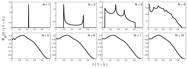
Figure 2: The radial distribution $P_{N}(r)$ for the representative case $\lambda=0.56$, with $N=1$, 2, 3, 4, 5, 6, 7, and 10 steps (upper left to lower right).

Figure 2 shows the radial distribution for $\lambda\approx\lambda_{c}$ after a small number of steps to provide a sense for the convergence rate to the asymptotic form. For convenience in putting many panels on the same scale, we typically plot the distribution $P(r)r_{\rm max}$ versus $r/r_{\rm max}$, where $r_{\rm max}=(1-\lambda)^{-1}$ is the maximal displacement of the infinite walk. Already by $N=7$ steps, the probability distribution is visually indistinguishable from its asymptotic form. While $P(r)$ varies smoothly as a function of $\lambda$, the position of the global maximum changes discontinuously from being peaked at $r>0$ to being peaked at $r=0$ as $\lambda$ increase beyond a critical value $\lambda_{c}(r)$. The single-coordinate distribution $P(x)$ exhibits a transition from multimodality to unimodality that somewhat resembles the transition for $P(r)$, but is more complex in its microscopic details.

Conventionally, the distribution of the displacment factorizes into a product of single-coordinate distribution, from which the radial distribution follows easily. However, in contrast to the classic Pearson walk in which the length of each step is the same, the probability distribution for the shrinking Pearson walk no longer factorizes as $P(\mathbf{r})=P(x)P(y)$. The differences between the radial and single-coordinate distributions arise because there is a non-trivial correlation between steps in orthogonal directions. If the endpoint of the walk is close to its maximum possible value in, say, the $x$-direction, then the displacement in the $y$-direction is necessarily small, and vice versa.

It is worth emphasizing that it is not practical to accurately determine the probability distribution of the Pearson random walk with shrinking steps by straightforward simulations. As we shall see, the nature of the transition in $P(x)$ is delicate. It would require a prohibitively large number of walks, or a prohibitively fine spatial grid in an exact enumeration method, to obtain sufficient accuracy to resolve these subtle features. For this reason, we employ an alternative approach that is based on calculating the Fourier transform of the probability distribution — which can be done exactly by elementary methods — and then inverting this transform by the highly accurate Van Deun and Cools vdc algorithm.

III Fourier Transform Solution of the Probability Distribution

III.1 Single-Coordinate Distribution

We first study the distribution of the (horizontal) $x$ coordinate. To obtain the distribution of $x$ after $N$ steps, $P_{N}(x)$, we start with the Chapman-Kolmogorov equation W94 that relates $P_{N}(x)$ to $P_{N-1}(x)$,

$$P_{N}(x)=\int dx^{\prime}\>P_{N-1}(x^{\prime})\,q_{N}(x-x^{\prime}),$$ (2)

where $q_{N}(w)$ is the probability of making a displacement whose horizontal component equals $w$ at the $N^{\rm th}$ step. Equation (2) states that to reach a point whose horizontal component equals $x$ after $N$ steps, the walk must first reach a point with horizontal component $x^{\prime}$ in $N-1$ steps and then hop from $x^{\prime}$ to $x$ at the $N^{\rm th}$ step.

We now introduce the Fourier transforms

$$P_{N}(k)=\int dx\>P_{N}(x)\>e^{ikx}~{},\qquad\mathrm{and}\qquad q_{N}(k)=\int dx\>q_{N}(x)\>e^{ikx}~{},$$

to recast the convolution in Eq. (2) as the product $P_{N}(k)=P_{N-1}(k)\,q_{N}(k)$. This equation has the formal solution

$$P_{N}(k)=P_{0}(k)\prod_{n=0}^{N}q_{n}(k)=\prod_{n=0}^{N}q_{n}(k)\,.$$ (3)

The latter equality applies for a walk that begins at the origin, so that $P_{0}(k)=1$. Now $q_{n}(x)$ may be obtained by transforming from the uniform distribution of angles to the distribution of the horizontal coordinate in a single step by using the relation

$$q_{n}(x)\,dx=q_{n}(\theta)\,d\theta=\frac{d\theta}{2\pi}~{},$$ (4)

together with $x=\lambda^{n-1}\cos\theta$, to give

$$q_{n}(x)=\frac{1}{\pi}\frac{1}{\sqrt{\lambda^{2(n-1)}-x^{2}}}~{}.$$ (5)

Although the distribution of angles is uniform, the single-step distribution for the $x$-coordinate at the $n^{\rm th}$ step has a “smile” appearance, with maxima at $x=\pm\lambda^{n-1}$ and a minimum at $x=0$. The probability distribution of the horizontal coordinate after $N$ steps is a convolution of these smile functions at different spatial scales. It is this superposition that gives $P(x)$ its rich properties for $\lambda\approx\lambda_{c}$.

Using the transformation between $x$ and $\theta$ in Eq. (4), the Fourier transform of the single-step probability is

$$q_{n}(k)=\int dx\>q_{n}(x)\>e^{ikx}=\frac{1}{2\pi}\int_{0}^{2\pi}d\theta\,e^{ik\lambda^{n-1}\cos\theta}=J_{0}(k\lambda^{n-1})\,,$$ (6)

where $J_{0}$ is the Bessel function of the first kind of order zero. This result relies on a standard representation of the Bessel function as a Fourier integral AS . Thus the Fourier transform of the probability distribution in Eq. (3) may be expressed as the finite product of Bessel functions

$$P_{N}(k)=\prod_{n=0}^{N-1}J_{0}(k\lambda^{n})\,.$$ (7)

To calculate $P_{N}(x)$ requires inverting the Fourier transform,

$$P_{N}(x)=\frac{1}{2\pi}\int_{-\infty}^{\infty}dk\>e^{-ikx}P_{N}(k)=\frac{1}{\pi}\int_{0}^{\infty}dk\>\cos kx\prod_{n=0}^{N-1}J_{0}(k\lambda^{n}),$$ (8)

where we use the fact that $P_{N}(k)$ is even in $k$ to obtain the second equality.

Each of the factors $J_{0}$ in the product in Eq. (8) is an oscillatory function of $k$, and the product itself oscillates more rapidly as the number of terms $N$ increases. The evaluation of integrals with such rapidly oscillating integrands has been the subject of considerable research oss ; in particular, integrals of products of Bessel functions appear in nuclear physics b3 , quantum field theory b1 , scattering theory b2 , and speech enhancement software b4 . Recently, Van Duen and Cools vdc developed an algorithm that can numerically calculate integrals of power laws multiplied by a product of Bessel functions of the first kind quickly and with absolute errors of the order of $10^{-16}$. We use their algorithm to compute the probability distribution $P_{N}(x)$ with this degree of accuracy. To implement their approach, we first write AS1

$$\cos z=\sqrt{\frac{\pi}{2z}}\left(\frac{1}{\sqrt{z}}\>J_{1/2}(z)-\sqrt{z}\>J_{3/2}(z)\right)$$

to express the right-hand side of Eq.(8) in terms of products of Bessel functions and a power law only. With this preliminary, we can directly apply the Van Duen-Cools algorithm to determine $P_{N}(x)$ accurately.

III.2 Radial Distribution

For the distribution of the radial coordinate $r$, $P_{N}(r)$, we again start with the Chapman-Kolmogorov equation W94

$$P_{N}(r)=\int d\mathbf{r}^{\prime}\>P_{N-1}(\mathbf{r}^{\prime})\mathcal{Q}_{N}(\mathbf{r}-\mathbf{r}^{\prime}),$$ (9)

where $\mathcal{Q}_{N}(\mathbf{z})$ is the probability that the walk makes a vector displacement $\mathbf{z}$ at the $N^{\rm th}$ step, and we use the angular symmetry of the walk to write $P_{N}$ as a function of only the magnitude of the displacement. Since all angles for the $N^{\text{th}}$ step are equiprobable,

$$\mathcal{Q}_{N}(\mathbf{r})=\frac{1}{2\pi r}\>\delta(\lambda^{N-1}-|\mathbf{r}|),$$ (10)

where $\delta(x)$ is the Dirac delta function. Once again, we use the Fourier transform to reduce the convolution in Eq. (9) to a product. This recursion has the solution

$$P_{N}(k)=P_{0}(\mathbf{k})\prod_{n=0}^{N-1}J_{0}(k\lambda^{n})=\prod_{n=0}^{N-1}J_{0}(k\lambda^{n})\,,$$ (11)

with the last equality appropriate for a walk that starts from the origin. While Eqs. (7) and (11) are identical, the corresponding distributions in real space are distinct. To obtain $P_{N}(r)$, we must calculate

$$P_{N}(\mathbf{r})=\frac{1}{(2\pi)^{2}}\int d\mathbf{k}\>e^{-i\mathbf{k}\cdot\mathbf{r}}P_{N}(\mathbf{k})\,.$$ (12)

Since $P_{N}(\mathbf{k})$ is a function of the magnitude of $\mathbf{k}$ only, we can write the integration in polar coordinates and perform the angular integration to obtain the spherically symmetric result

$$P_{N}(r)=\frac{1}{2\pi}\int_{0}^{\infty}dk\>k\>J_{0}(kr)\prod_{n=0}^{N-1}J_{0}(k\lambda^{n})\,.$$ (13)

In this Bessel product form, we can again apply the Van Duen-Cools algorithm vdc to invert this Fourier transform numerically.

IV THE PROBABILITY DISTRIBUTIONS

We numerically integrate Eq. (8) by the Van Duen-Cools algorithm to give the single-coordinate probability distribution $P_{N}(x)$ whose evolution as a function of $\lambda$ is schematically illustrated in Fig. 3. Notice that there is a value $\lambda\approx 0.5567$ for which the curvature at the origin vanishes. However, at this value of $\lambda$ the global maximum of the $P(x)$ is not at the origin. Thus points where $P^{\prime\prime}(x)=0$ do not help locate the global extrema of the probability distribution and we must resort to the numerical integration.

Since the individual step lengths decay exponentially with $N$, the finite-$N$ distribution $P_{N}(x)$ quickly converges to its asymptotic $N\to\infty$ form. For example, for $\lambda=0.56$ (close to $\lambda_{c}(x)$), the displacement of the walk after 15 steps is within $10^{-5}$ of its final endpoint. Hence the probability distribution is visually indistinguishable from the asymptotic distribution on the scale of the plots in Fig. 4. We always use values of $N$ for each $\lambda$ to ensure that $x_{N}$ is within $10^{-5}$ of its final displacement.

Figure 3: Schematic and not to scale form of $P(x)$ for increasing $\lambda$ near $\lambda_{c}$ (bottom to top). For $\lambda\approx 0.5567<\lambda_{c}$ the curvature at the origin becomes positive, while at $\lambda=\lambda_{c}$ the location of the maximum in $P(x)$ changes discontinuously. For $\lambda\to 1$, $P(x)$ approaches a Gaussian.

For small $\lambda$, $P(x)$ resembles the smile distribution of the single-step distribution in Eq. (5). As $\lambda$ approaches $\lambda_{c}$ from below, the minimum at the origin gradually fills in and disappears for $\lambda\approx 0.56$. For $\lambda>\lambda_{c}$, the distribution develops a maximum at the origin that becomes increasingly Gaussian in appearance as $\lambda\to 1$.

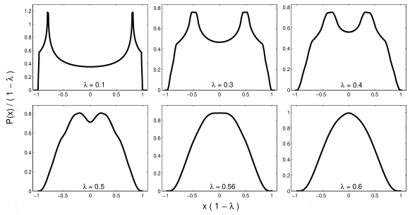
Figure 4: Scaled $x$-coordinate distribution for the shrinking Pearson walk in two dimensions for $\lambda=0.1$, 0.3, 0.4, 0.5, 0.56, and 0.6 (upper left to lower right).

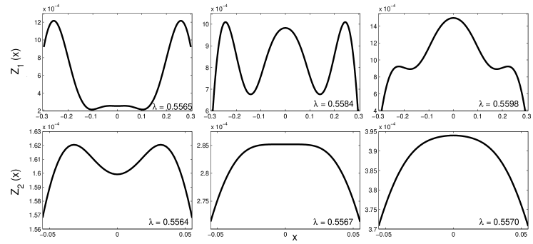
Figure 5: The single-coordinate distribution at highly-magnified scales. Top line: $Z_{1}(x)\equiv P(x)-0.387$ for $\lambda=0.5565$, 0.5584, and 0.5598. Bottom line: $Z_{2}(x)\equiv P(x)-0.3870562$ for $\lambda=0.5564$, 0.5567, and 0.5570.

Unexpectedly, $P(x)$ has multiple tiny maxima near the origin, that are not visible on the scale of Fig. 4, as $\lambda$ passes through $\lambda_{c}$. The Van Duen-Cools algorithm is essential to obtain sufficient numerical accuracy to observe these anomalies. The top line of Fig. 5 shows the quantity $Z_{1}(x)\equiv P(x)-0.387$, with the vertical scale magnified by $10^{3}$ to expose the minute variations of $P(x)$. At this magnification, one can see the birth of a maximum in $P(x)$ at the origin that gradually overtakes the secondary maxima near $|x|\approx 0.2$. Consequently, the location of the global maximum of $P(x)$ jumps discontinuously from a non-zero value to zero at $\lambda=\lambda_{c}(x)\approx 0.5584558\pm 0.0000003$ (as illustrated by the middle panel on the top line of Fig. 5, which shows $P(x)$ for $\lambda_{c}-\lambda\sim\mathcal{O}\left(10^{-5}\right)$).

At a still higher resolution, the nearly flat distribution near $x=0$ at magnification $10^{3}$ is actually oscillatory at magnification $10^{5}$ (Fig. 5 lower line). We see that the small maximum that is born when $\lambda$ passes through approximately 0.5565 (Fig. 5, upper left) actually contains an even smaller dimple that disappears when $\lambda\gtrsim 0.5567$ (middle panel in the lower line of Fig. 5). To highlight this fine-scale anomaly, we plot, in the lower line of Fig. 5, the quantity $Z_{2}(x)\equiv P(x)-0.3870562$ for three $\lambda$ values that are very close to $\lambda_{c}$. Intriguingly, we do not find evidence of additional anomalous features at a still finer scale of resolution.

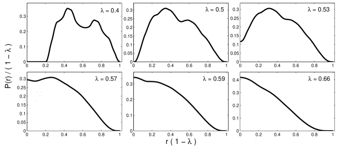
Figure 6: The radial distribution for the shrinking Pearson walk in two dimensions for the cases $\lambda=0.40$, 0.50, 0.53, 0.57, 0.59, and 0.66.

We also use the Van Duen-Cools algorithm to numerically integrate Eq. (13) and determine the radial distribution $P_{N}(r)$. For a small number of steps $N$, $P_{N}(r)$ changes significantly with each additional step, as was illustrated in Fig. 2. Once the number of steps becomes of the order of 10, however, $P_{N}(r)$ is very close to the asymptotic $P(r)$ for $\lambda\approx\lambda_{c}(r)$. The transition behavior in $P(r)$ turns out to be much simpler than that for $P(x)$. For $P(r)$, a peak gradually develops at the origin, while the peak $r>0$ gradually recedes as $\lambda$ increases. Thus as $\lambda$ passes through $\lambda_{c}(r)$, the location of the global peak of $P(r)$ discontinuously jumps to zero (Fig. 6). We do not find evidence of fine-scale anomalies in the radial distribution as $\lambda$ passes through $\lambda_{c}(r)$.

V HIGHER DIMENSIONS

The approach developed for two dimensions can be straightforwardly extended to higher spatial dimensions. For the radial distribution in $d$ dimensions, the single-step distribution $\mathcal{Q}_{N}(r)$ is now

$$\mathcal{Q}_{N}(r)=\frac{1}{r^{d-1}\Omega_{d}}\>\delta\left(r-\lambda^{N}\right),$$ (14)

where $\Omega_{d}=2\pi^{d/2}/\>\Gamma(d/2)$ is the surface area of the unit hypersphere in $d$ dimensions and $r=|\mathbf{r}|$ is the radial distance. The corresponding Fourier transform is AS2

$$\mathcal{Q}_{N}(k) = \Omega_{d}^{-1}\int\text{d}\mathbf{r}\ \frac{\delta\left(r-\lambda^{n}\right)}{r^{d-1}}\>e^{i\mathbf{k}\cdot\mathbf{r}},$$ (15)

$$= \frac{\Gamma\left(\frac{d}{2}\right)}{\Gamma\left(\frac{1}{2}\right)\>\Gamma\left(\frac{d-1}{2}\right)}\int_{0}^{\pi}\text{d}\theta\>\sin^{d-2}\theta\>e^{ik\lambda^{N}\cos\theta}={}_{0}{F}{{}_{1}}(d/2,-k^{2}\lambda^{2N}/4),$$

where ${}_{0}F_{1}(a,z)$ is the confluent hypergeometric function. The Fourier transform $P_{N}(k)$ is then the product of Fourier transform of the single-step distributions, and its Fourier inverse gives $P_{N}(r)$. By integrating over the $d-2$ azimuthal angles, and then integrating over the polar angle $\theta$, as in Eq. (15), the formal solution is

$$P_{N}(r) = \frac{\Omega_{d-1}}{(2\pi)^{d}}\int dk\>k^{d-1}P_{N}(k)\int_{0}^{\pi}d\theta\>\sin^{d-2}\theta\>e^{-ikr\cos\theta},$$ (16)

$$= \frac{2^{1-d}}{\pi^{d/2}\Gamma(d/2)}\int_{0}^{\infty}dk\>k^{d-1}{}_{0}{F}{{}_{1}}(d/2,-k^{2}r^{2}/4)\>\>\prod_{n=0}^{N}{}_{0}{F}{{}_{1}}(d/2,-k^{2}\lambda^{2n}/4)\,.$$

Since ${}_{0}F_{1}(\nu+1,-(z/2)^{2})\propto(z/2)^{-\nu}J_{\nu}(z)$ AS2 , we can again numerically determine $P_{N}(r)$ by using the Van Duen-Cools algorithm. The result of this calculation is that the radial distribution undergoes a second-order transition at $\lambda_{c}$ in which the location of the single maximum continuously decreases to zero as $\lambda$ increases beyond $\lambda_{c}$.

The same formal approach can be used to calculate the distribution $P(x)$. This distribution now remains peaked at the origin for all values of $\lambda$. The physical origin of this property stems from the nature of the single-step distribution. The generalization of Eq. (5) is

$$q_{n}(x)\propto\left[\lambda^{2(n-1)}-x^{2}\right]^{(d-3)/2}~{}.$$

This function is flat for $d=3$ and peaked at the origin for $d>3$. Consequently, the convolution of these single-step distributions leads to $P_{N}(x)$ having a single peak at the origin.

VI DISCUSSION

We investigated the shrinking Pearson walk, where each step is in a random direction, while the length of the $n^{\rm th}$ step is $\lambda^{n-1}$, with $\lambda<1$. Because the step lengths are not identical, one of the defining conditions for the central limit theorem is violated. Consequently, there is no reason to expect that the probability distribution for this walk is Gaussian. We studied basic properties of the radial probability distribution, $P(r)$, and the distribution of a single coordinate, $P(x)$. Because a walk with a large displacement in one direction necessarily implies a small displacement in the orthogonal direction, $P(r)$ does not simply factorize as a product of single-coordinate distributions. The $P(r)$ and $P(x)$ are distinct distributions.

In two dimensions, the radial probability distribution of the shrinking Pearson walk changes from being peaked away from the origin to being peaked at the origin as the shrinking factor $\lambda$ increases beyond a critical value $\lambda_{c}(r)$. As this transition in $\lambda$ is passed, the location of the peak changes discontinuously from a non-zero value to $r=0$. In greater than two dimensions, there is a similar shape transition in the radial distribution, but now the location of the only peak goes to zero continuously as $\lambda$ increases beyond $\lambda_{c}(r)$.

The single-coordinate distribution $P(x)$ has peculiar features for the specific case of two dimensions. Visually, $P(x)$ becomes nearly flat at the origin for $\lambda\approx 0.5565$ (middle panel, bottom row of Fig. 4). However, at a higher degree of magnification, this nearly flat portion of the distribution exhibits fine-scale oscillations, with up to seven local extrema. Because additional oscillations can be resolved as the resolution is increased, it is tempting to speculate that arbitrarily many oscillations occur at progressively decreasing scales. To test for this possibility, we computed the first derivative $P_{N}^{\prime}(x)$ from Eq. (8), and looked for additional zeros in $P_{N}^{\prime}(x)$ as a function of $x$. Again employing the Van Duen-Cools algorithm, we find the $P_{N}(x)$ is strictly positive for $x$ in the range $5\times 10^{-8}$ to $10^{-4}$ when $\lambda=0.55672$, but is strictly negative in the same range of $x$ when $\lambda=0.55673$. Moreover, $P_{N}^{\prime}(x)$ appears to scale as $x^{1/2}$ in the range $5\times 10^{-8}<x<10^{-4}$, so we anticipate no additional zeros for $x\to 0$. This numerical test suggests that there are no additional oscillations in $P(x)$ beyond those revealed in Fig. 5.

We are grateful for financial support from DOE grant DE-FG02-95ER14498 (CAS) and NSF grant DMR0535503 and DMR0906504 (SR).

References

- (1) K. Pearson, Nature 72 294; 318; 342 (1905).
- (2) G. H. Weiss, Aspects and Applications of the Random Walk (North-Holland, Amsterdam, 1994).
- (3) B. Jessen and A. Wintner, Trans. Amer. Math. Soc. 38, 48–88 (1935); B. Kershner and A. Wintner, Amer. J. Math. 57, 541–548 (1935); A. Wintner, ibid. 57, 827–838 (1935).
- (4) P. Erdős, Amer. J. Math. 61, 974–976 (1939); P. Erdős, ibid. 62, 180–186 (1940).
- (5) A. M. Garsia, Trans. Amer. Math. Soc. 102, 409–432 (1962); A. M. Garsia, Pacific J. Math. 13, 1159–1169 (1963).
- (6) M. Kac, Statistical Independence in Probability, Analysis and Number Theory (Mathematical Association of America; distributed by Wiley, New York, 1959).
- (7) P. L. Krapivsky and S. Redner, Am. J. Phys. 72, 591–598 (2004).
- (8) Y. Peres, W. Schlag, and B. Solomyak, in Fractals and Stochastics II, edited by C. Bandt, S. Graf, and M. Zähle (Progress in Probability, Birkhauser, 2000), vol. 46, pp. 39–65.
- (9) E. Barkai and R. Silbey, Chem. Phys. Lett. 310, 287 (1999); Phys. Chem. B, 104, 342 (2000).
- (10) G. H. Weiss and J. E Kiefer, J. Phys. A 16, 489–495 (1983).
- (11) T. Rador, Phys. Rev. E 74 051105 (2006).
- (12) S. N. Majumdar and M. J. Kearney, Phys. Rev. E, 76, 031130 (2007).
- (13) M. Bazant, private communications. See, also lecture notes by M. Bazant for MIT course 18.366. The URL is <http://ocw.mit.edu/Ocw/Mathematics/18-366Fall-2006/CourseHome/>.
- (14) J. Van Deun and R. Cools, ACM Transactions on Mathematical Software 32 580–596 (2006); Comp. Phys. Comm. 178 578–590 (2008).
- (15) E. Ben-Naim, S. Redner, and D. ben-Avraham, Phys. Rev. A 45, 7207 (1992); D. ben-Avraham, F. Leyvraz, and S. Redner, Phys. Rev. A 45, 2315 (1992).
- (16) M. Abramowitz and I. A. Stegun Handbook of Mathematical Functions (Dover, New York, 1972). See 9.1.21.
- (17) See 10.1.1. anmd 10.1.11 in reference AS that gives the representation of in terms of Bessel functions.
- (18) See 9.1.20 and 9.1.69 in reference AS for the connection between the relevant Fourier integrals and the hypergeometric function.
- (19) See for example: L. N. G. Filon, Proc. Roy. Soc. Edinburgh 49 38-49 (1928), Y. L. Luke, Proc. Cambridge Phil. Soc. 50, 269–277 (1954), B. Gabutti, Math. Comp. 33, 1049-1057 (1979), G. A. Evans, Practical Numerical Integration, (Chaps. 3 and 4) (Wiley, New York, 1993).
- (20) S. Groote, J. G. Körner, and A. A. Pivovarov, Nucl. Phys. B 542, 515–547 (1999).
- (21) S. Davis, Class. Quantum Grav. 18, 3395–3425 (2001).
- (22) R. Gaspard and D. Alonso Ramirez, Phys. Rev. A 45, 8383–8397 (1992).
- (23) T. Lotter, C. Benien, and P. Vary, EURASIP Journal on Applied Signal Processing 11, 1147–1156 (2003).