Zero temperature phases of the frustrated J₁-J₂ antiferromagnetic spin-1/2 Heisenberg model on a simple cubic lattice

Abstract

At zero temperature magnetic phases of the quantum spin-$1/2$ Heisenberg antiferromagnet on a simple cubic lattice with competing first and second neighbor exchanges ($J_{1}$ and $J_{2}$) is investigated using the non-linear spin wave theory. We find existence of two phases: a two sublattice Néel phase for small $J_{2}$ (AF), and a collinear antiferromagnetic phase at large $J_{2}$ (CAF). We obtain the sublattice magnetizations and ground state energies for the two phases and find that there exists a first order phase transition from the AF-phase to the CAF-phase at the critical transition point, $p_{c}=0.28$. Our results for the value of $p_{c}$ are in excellent agreement with results from Monte-Carlo simulations and variational spin wave theory. We also show that the quartic $1/S$ corrections due spin-wave interactions enhance the sublattice magnetization in both the phases which causes the intermediate paramagnetic phase predicted from linear spin wave theory to disappear.

I Introduction

Frustrated quantum Heisenberg magnets with competing nearest neighbor (NN) and next-nearest-neighbor (NNN) antiferromagnet (AF) exchange interactions, $J_{1}$ and $J_{2}$ respectively, have been under intense investigation both theoretically and experimentally in condensed matter physics for more than a decade. Diep (2004) At low temperatures these systems exhibit new types of magnetic order and novel quantum phases. Diep (2004); Sachdev (2001, ) A well-known example is the quantum spin-$1/2$ antiferromagnetic $J_{1}-J_{2}$ model on a square lattice, which has been studied extensively by various analytical and numerical methods. Rastelli et al. (1979); Reatto and Tassi (1985); Barabanov and Starykh (1990); Sachdev (1992a); Dotsenko and Sushkov (1994); Chubukov (1992a); Gelfand et al. (1989); Sushkov et al. (2001); Weihong et al. (1999); Singh et al. (1999); Irkhin et al. (1992) For this two-dimensional square lattice system with $J_{2}=0$ the ground state is antiferromagnetically ordered at zero temperature. Addition of next nearest neighbor interactions induces a strong frustration and break the antiferromagnetic (AF) order. The competition between the NN and NNN interactions for the square lattice is characterized by the frustration parameter $p=J_{2}/J_{1}$. It has been found that a disordered quantum spin liquid phase exists between $p_{1c}\approx 0.38$ and $p_{2c}\approx 0.60$. For $p<p_{1c}$ the square lattice is AF-ordered whereas for $p>p_{2c}$ a collinear phase emerges. In the collinear state the NN spins have a parallel orientation in the vertical direction and antiparallel orientation in the horizontal direction or vice versa. The nature of phase transition from AF-ordered state to disordered state at $p_{1c}$ is of second order and from the disordered state to the collinear state at $p_{2c}$ is of first order.

The properties of quantum magnets depend strongly on the lattice dimensionality since the tendency to order is more pronounced in three dimensional (3D) systems than in the lower dimensional systems. Furthermore, in 3D the available phase space is more and we expect quantum fluctuations to play a lesser role as compared to 1D and 2D. In 1D and 2D the available phase space is limited and quantum fluctuations play a dominant role in determining the quantum critical points. Despite this fact a magnetically disordered phase has been observed in frustrated 3D systems such as the Heisenberg AF on the pyrochlore lattice Canals and Lacroix (1998) or on the stacked kagome lattice Fak et al. (2008); Sachdev (1992b); Chubukov (1992b); Harris et al. (1992). Studies on the Heisenberg AF on the pyrochlore lattice (a geometrically frustrated system) have revealed the existence of a spin liquid state. Canals and Lacroix (1998) On the other hand, for the 3D J1-J2 model on the body-centered cubic (BCC) lattice there are no signs of an intermediate quantum paramagnetic phase at zero temperature. Oitmaa and Zheng (2004); Schmidt et al. (2002); Majumdar and Datta (2009) For the BCC lattice competing interactions and not lattice geometry generates the frustration. This comparison illustrates how the magnetic phase diagram may dramatically change based on whether the frustration is generated by competing interactions or by geometry.

Most of the efforts on quantum 3D magnets have primarily focused on geometrically frustrated lattices. Diep (2004); Sachdev (2001) There exists some computationalAzaria (1986); Derrida et al. (1979, 1980); Lallemand et al. (1985); Karchev (2008, 2009); Banavar et al. (1979); Oitmaa and Zheng (2004); Schmidt et al. (2002); Oguchi et al. (1985); Ignatenko et al. (2008); Diep and Kawamura (1989); Ader (2002) and very few analytical studiesVillain (1959, 1977); Banavar et al. (1979); Majumdar and Datta (2009) of the magnetic phase diagrams and magnetic order of spin-$1/2$ Heisenberg AF on 3D lattices where on the study of magnetic phase diagrams and magnetic order of spin-$1/2$ Heisenberg AF on 3D lattices where competing interactions induce frustration. Villain (1959, 1977); Azaria (1986); Derrida et al. (1979, 1980); Lallemand et al. (1985); Karchev (2008, 2009); Banavar et al. (1979); Oitmaa and Zheng (2004); Schmidt et al. (2002); Majumdar and Datta (2009); Oguchi et al. (1985); Ignatenko et al. (2008); Diep and Kawamura (1989); Ader (2002)

Very few analytical and numerical results exist for the the frustrated $J_{1}-J_{2}$ isotropic Heisenberg model on a simple cubic lattice. Pinettes and Diep (1998); Diep et al. (1985); Irkhin et al. (1992); Kishi and Kubo (1991) This model has been studied previously using Monte Carlo simulation Pinettes and Diep (1998), variational spin wave theory Kishi and Kubo (1991), and modified spin wave theory Irkhin et al. (1992). In a recent work the critical properties of the 3D anisotropic quantum spin-$1/2$ model on a simple cubic (SC) lattice has been investigated within the framework of the differential operator technique and by using an effective field theory in a two-spin cluster. Viana et al. (2008) The study revealed that at zero temperature there is a AF-lamellar (first order) phase transition. The motivation for the present work is to investigate the zero temperature phases of this model in the framework of non-linear spin wave theory (NLSWT) and to obtain the critical transition points of this model. Also we will compare our results from NLSWT with the prediction from the linear spin wave theory (LSWT).

The paper is organized as follows. In Section II we set-up the Hamiltonian for the spin-$1/2$ Heisenberg AF on the SC lattice. The classical ground state configurations of the model and the different phases are then discussed. In Section III we map the spin Hamiltonian to the Hamiltonian of interacting bosons and develop the NLSWT sublattice magnetization and energy expressions. The sublattice magnetizations and the ground state energies for the two phases are numerically calculated and the results are plotted and discussed in Section IV. Finally we summarize our findings in Section V.

II Classical Ground State Configurations

The Hamiltonian for a spin-$1/2$ Heisenberg antiferromagnet with first and second neighbor interactions on a simple cubic (SC) lattice is

$$H=\frac{1}{2}J_{1}\sum_{\langle ij\rangle}{\bf S}_{i}\cdot{\bf S}_{j}+\frac{1}{2}J_{2}\sum_{[ij]}{\bf S}_{i}\cdot{\bf S}_{j}.$$ (1)

$J_{1}$ is the NN and $J_{2}$ is the frustrating NNN (which are along the face diagonals of the cube) exchange constants. Both couplings are considered antiferromagnetic, i.e. $J_{1},J_{2}>0$. For the SC lattice the number of nearest and next-nearest neighbors are $z_{1}=6$ and $z_{2}=12$.

The limit of infinite spin, $S\rightarrow\infty$, corresponds to the classical Heisenberg model. We assume that classically the spin configurations of the system are described by $S_{i}=S{\bf u}e^{i{\bf q}\cdot{\bf r_{i}}}$, where ${\bf u}$ is a vector expressed in terms of an arbitrary orthonormal basis and ${\bf q}$ defines the relative orientation of the spins on the lattice. The classical ground state energy of the lattice in terms of the frustration parameter, p, is given by

$$E_{\bf k}/NJ_{1}=\frac{1}{2}S^{2}z_{1}[\gamma_{1{\bf k}}+p\gamma_{2{\bf k}}],$$ (2)

with the structure factors

$$\gamma_{1{\bf k}} = \frac{1}{3}\Big{[}\cos(k_{x})+\cos(k_{y})+\cos(k_{z})\Big{]},$$ (3)

$$\gamma_{2{\bf k}} = \frac{1}{3}\Big{[}\cos(k_{x})\cos(k_{y})+\cos(k_{y})\cos(k_{z})+\cos(k_{z})\cos(k_{x})\Big{]},$$ (4)

where we define the parameter of frustration as $p=z_{2}J_{2}/z_{1}J_{1}$. not The wave-vectors along the $x$, $y$, and $z$ directions are denoted by $k_{x},k_{y}$, and $k_{z}$. The number of lattice sites are given by $N$ and we have set the lattice spacing $a=1$.

At zero temperature the classical ground state (GS) for the SC lattice can be characterized by the values of $p$. $p=0$ corresponds to the unfrustrated case (only AF interactions between NN). For $p<1/2$ or $J_{2}/J_{1}<1/4$, there is a single minimum in energy $E_{0}/NJ_{1}=-3S^{2}(1-p)$ for the wave-vector $(\pm\pi,\pm\pi,\pm\pi)$. They correspond to the classical two sublattice Néel state (AF phase) where spins in A and B-sublattices point in opposite directions [Fig. 1(a)].

For $p>1/2$ apart from the global rotation the classical ground state has an infinite degeneracy – the frustration is uniformly distributed on all the spins, causing a non-collinear GS with very large degeneracy. In general, the GS for $p>1/2$ can be decomposed into two NNN tetrahedra. The spin configurations in each of these two NNN tetrahedra can be characterized by two angles $\theta$ and $\phi$. This results in a four sublattice $A,B,C,D$ [Fig. 1(b)] antiferromagnetic structure. Out of these infinite possibilities there are three collinear configurations (one line up, one line down). The wave-vectors corresponding to these collinear states are $(\pi,\pi,0),\;(\pi,0,\pi),\;(0,\pi,\pi)$. The classical GS energy for these states is $E_{0}/NJ_{1}=-S^{2}(1+p)$. Thermal or quantum fluctuations lift these degeneracies and select specific discrete states and it has been conjectured that thermal or quantum disorder favors collinear states (order by disorder). Shender (1982); Henley (1989) The four fold rotational symmetry of the lattice is spontaneously broken in this state. By employing a spin wave theory based on the general four sublattice mean field ground state it has been shown that the quantum fluctuations stabilize a collinear spin ordering. Kubo and Kishi (1991) Quantum Monte Carlo simulations on the frustrated SC lattice for $p>1/2$ also confirm this conjecture. Pinettes and Diep (1998) In the present article, for $p>1/2$, we consider the system to be in one of these three collinear configurations (collinear antiferromagnet or CAF).

$p=1/2$ corresponds to the case where both $J_{1}$ and $J_{2}$ compete – causing frustration in the system. This critical value $p_{\rm class}=0.5$ is the classical phase transition point where a phase transition from AF to CAF phase occurs. In this work we will investigate the role of quantum fluctuations in the two different phases (AF and CAF) of the model and how these fluctuations shift the critical transition point.

III Self-consistent non-linear spin wave theory

The Hamiltonian in Eq. 1 can be mapped into an equivalent Hamiltonian of interacting bosons by transforming the spin operators to bosonic operators $a,a^{\dagger}$ and $b,b^{\dagger}$ using the well-known Holstein-Primakoff transformations. For the AF-phase ($J_{2}<J_{1}$) the operators $a,a^{\dagger}$ and $b,b^{\dagger}$ are for the $A$ and $B$ sublattices. On the other hand for the CAF phase ($J_{2}>J_{1}$) we have used the operators $a,a^{\dagger}$ and $b,b^{\dagger}$ for the up and down spin configurations.

$$S_{Ai}^{+} \approx \sqrt{2S}\Big{(}1-\frac{a_{i}^{\dagger}a_{i}}{4S}\Big{)}a_{i},\;\;S_{Ai}^{-}\approx\sqrt{2S}a_{i}^{\dagger}\Big{(}1-\frac{a_{i}^{\dagger}a_{i}}{4S}\Big{)},$$

$$S_{Ai}^{z} = S-a^{\dagger}_{i}a_{i},$$

$$S_{Bj}^{+} \approx \sqrt{2S}b_{j}^{\dagger}\Big{(}1-\frac{b_{j}^{\dagger}b_{j}}{4S}\Big{)},\;\;S_{Bj}^{-}\approx\sqrt{2S}\Big{(}1-\frac{b_{j}^{\dagger}b_{j}}{4S}\Big{)}b_{j},$$

$$S_{Bj}^{z} = -S+b^{\dagger}_{j}b_{j},$$ (5)

In these transformations we only kept terms up to the order of $1/S$. Next using the Fourier transforms

$$a_{i}=\sqrt{\frac{2}{N}}\sum_{\bf k}e^{-i{\bf k\cdot R_{i}}}a_{\bf k},\;\;\;b_{j}=\sqrt{\frac{2}{N}}\sum_{\bf k}e^{-i{\bf k\cdot R_{j}}}b_{\bf k},$$

the real space Hamiltonian is transformed to the ${\bf k}$-space Hamiltonian. In the following two sections we study the cases $J_{2}<J_{1}$ and $J_{2}>J_{1}$ separately.

III.0.1 $J_{2}<J_{1}$: AF phase

In this phase the classical ground state is the two-sublattice Néel state [Fig. 1(a)]. For the NN interaction, spins in $A$ sublattice interacts with spins in $B$ sublattice and vice versa. On the other hand the NNN exchange $J_{2}$ connects spins on the same sublattice, $A$ with $A$ and $B$ with $B$. Substituting equations (5) into (1), the ${\bf k}$-space Hamiltonian takes the form:

$$H=H^{(0)}+H^{(2)}+H^{(4)}.$$ (6)

The classical ground state energy $H^{(0)}$ and the quadratic terms $H^{(2)}$ are

$$H^{(0)} = -\frac{1}{2}NJ_{1}S^{2}z_{1}(1-p),$$ (7)

$$H^{(2)} = J_{1}Sz_{1}\sum_{\bf k}\Big{[}A^{(1)}_{0{\bf k}}(a_{\bf k}^{\dagger}a_{\bf k}+b_{\bf k}^{\dagger}b_{\bf k})+B^{(1)}_{0{\bf k}}(a^{\dagger}_{\bf k}b^{\dagger}_{-\bf k}+a_{-\bf k}b_{\bf k})\Big{]}.$$ (8)

with the coefficients $A^{(1)}_{0{\bf k}}$ and $B^{(1)}_{0{\bf k}}$ defined as

$$A^{(1)}_{0{\bf k}} = 1-p(1-\gamma_{2{\bf k}}),$$ (9)

$$B^{(1)}_{0{\bf k}} = \gamma_{1{\bf k}}.$$ (10)

The quartic terms in the Hamiltonian $H^{(4)}$ involve interactions between $A-B$ (for NN terms) and $A-A,\;B-B$ (for NNN terms) sublattices. The Hamiltonian for these interaction are stated in Appendix A, Eq. 26. These terms are evaluated by applying the Hartree-Fock decoupling process. The contributions of the decoupled quartic terms to the harmonic Hamiltonian in Eq. 8 are to redefine the values of $A^{(1)}_{0{\bf k}}$ and $B^{(1)}_{0{\bf k}}$ which are now

$$A^{(1)}_{\bf k} = \Big{(}1-\frac{u_{1}+v_{1}}{S}\Big{)}-p[1-\gamma_{2{\bf k}}]\Big{(}1-\frac{u_{1}-w_{1}}{S}\Big{)},$$ (11)

$$B^{(1)}_{\bf k} = \gamma_{1{\bf k}}\Big{(}1-\frac{u_{1}+v_{1}}{S}\Big{)},$$ (12)

$$\omega^{(1)}_{\bf k} = \sqrt{\Big{(}A^{(1)}_{\bf k}\Big{)}^{2}-\Big{(}B^{(1)}_{\bf k}\Big{)}^{2}}.$$ (13)

The coefficients $u_{1},v_{1}$ and $w_{1}$ are in Appendix A. They are evaluated self-consistently from equations (11), (12), (27)–(29).

The quartic corrections to the ground state energy is calculated from the four-boson averages. In the leading order they are decoupled into the bilinear combinations (equations (27) – (29)) using Wick’s theorem. The corresponding four boson terms are,

$$\langle a^{\dagger}_{i}a_{i}b^{\dagger}_{j}b_{j}\rangle = u_{1}^{2}+v_{1}^{2},\;\;\;\langle a^{\dagger}_{i}b^{\dagger}_{j}b_{j}b_{j}\rangle=2u_{1}v_{1},$$

$$\langle a^{\dagger}_{i}a_{i}a_{i}b_{j}\rangle = 2u_{1}v_{1},\;\;\;\langle a^{\dagger}_{i}a_{i}a_{j}^{\dagger}a_{j}\rangle=u_{1}^{2}+w_{1}^{2},$$ (14)

$$\langle a_{i}a_{j}^{\dagger}a_{j}^{\dagger}a_{j}\rangle = 2u_{1}w_{1},\;\;\;\langle a^{\dagger}_{i}a_{i}a_{i}a_{j}^{\dagger}\rangle=2u_{1}w_{1}.$$

This yields the ground state energy correction from the quartic terms:

$$\delta E^{(4)}=-\frac{1}{2}NJ_{1}z_{1}\big{[}(u_{1}+v_{1})^{2}-p(u_{1}-w_{1})^{2}\big{]}.$$ (15)

Adding all the corrections together the ground state energy takes the form

$$E/NJ_{1} = -\frac{1}{2}z_{1}S(S+1)(1-p)+\frac{1}{2}z_{1}S\Big{[}\frac{2}{N}\sum_{\bf k}\omega^{(1)}_{\bf k}\Big{]}$$ (16)

$$+ \frac{1}{2}z_{1}\big{[}(u_{1}+v_{1})(1-u_{1}-v_{1})-p(u_{1}-w_{1})(1-u_{1}+w_{1})\big{]}$$

and the average sublattice magnetization $\langle S_{\alpha}\rangle$ is given by

$$\langle S_{\alpha}\rangle=S\Big{[}1-\frac{1}{2S}\Big{\{}\frac{2}{N}\sum_{\bf k}\frac{A^{(1)}_{\bf k}}{\omega^{(1)}_{\bf k}}-1\Big{\}}\Big{]}.$$ (17)

Using equations (11)–(13), we numerically evaluate $E/NJ_{1}$ and $\langle S_{\alpha}\rangle$.

III.0.2 $J_{2}>J_{1}$: CAF phase

The classical ground state for $J_{2}>J_{1}$ is considered to be in one of the three collinear states [Fig. 1(b)]. For NN and NNN exchanges there are $A-B$, $A-C$, $A-D$, $B-C$, $B-D$, and $C-D$ interactions between the four sublattices [See Fig. 1(b)]. Considering all their contributions together up to the quadratic terms the harmonic Hamiltonian takes the same form as before with

$$H^{(0)} = -\frac{1}{6}NJ_{1}S^{2}z_{1}(1+p),$$ (18)

$$A^{(2)}_{0{\bf k}} = \frac{1}{3}(1+\cos k_{z})+\frac{1}{3}p(1+\cos k_{x}\cos k_{y}),$$ (19)

$$B^{(2)}_{0{\bf k}} = \frac{1}{3}(\cos k_{x}+\cos k_{y})(1+p\cos k_{z}).$$ (20)

The quartic terms in the Hamiltonian for this case are shown in Appendix B. These terms are decoupled and evaluated in the same way as before. The renormalized values of the coefficients $A^{(2)}_{\bf k}$ and $B^{(2)}_{\bf k}$ are

$$A^{(2)}_{\bf k} = A^{(2)}_{0{\bf k}}+\frac{1}{3S}\big{[}({\overline{u}}-{\overline{w}_{z}})(1-\cos k_{z})-2({\overline{u}}+{\overline{v}_{1}})$$ (21)

$$+ p\big{\{}({\overline{u}}-{\overline{w}_{1}})(1-\cos k_{x}\cos k_{y})-2({\overline{u}}+{\overline{v}_{2}})\big{\}}\big{]},$$

$$B^{(2)}_{\bf k} = B^{(2)}_{0{\bf k}}-\frac{1}{3S}\big{\{}({\overline{u}}+{\overline{v}_{1}})+p({\overline{u}}+{\overline{v}_{2}})\cos k_{z}\big{\}}(\cos k_{x}+\cos k_{y}),$$ (22)

$$\omega^{(2)}_{\bf k} = \sqrt{\Big{(}A^{(2)}_{\bf k}\Big{)}^{2}-\Big{(}B^{(2)}_{\bf k}\Big{)}^{2}}.$$ (23)

The coefficients ${\overline{u}},{\overline{v}_{1}},{\overline{v}_{2}},{\overline{w}_{1}},{\overline{w}_{z}}$ are in Appendix B. As before these coefficients are calculated self-consistently from equations (21)–(23) and (31)–(37). The quartic correction to the ground state energy (following the same Hartree-Fock decoupling process as done in the AF-case) is

$$\delta E^{(4)}=-\frac{1}{6}NJ_{1}z_{1}\big{[}2({\overline{u}}+{\overline{v}_{1}})^{2}-({\overline{u}}-{\overline{w}_{z}})^{2}+2p({\overline{u}}+{\overline{v}_{2}})^{2}-p({\overline{u}}-{\overline{w}_{2}})^{2}\big{]}.$$ (24)

Combining all these corrections, the ground state energy takes the following form:

$$E/NJ_{1} = -\frac{1}{6}z_{1}S(S+1)(1+p)+\frac{1}{2}z_{1}S\Big{[}\frac{2}{N}\sum_{\bf k}\omega^{(2)}_{\bf k}\Big{]}$$ (25)

$$- \frac{1}{6}z_{1}\big{[}({\overline{u}}-{\overline{w}_{z}})-2({\overline{u}}+{\overline{v}_{1}})+p({\overline{u}}-{\overline{w}_{1}})-2p({\overline{u}}+{\overline{v}_{2}})\big{]}$$

$$- \frac{1}{6}z_{1}\big{[}2({\overline{u}}+{\overline{v}_{1}})^{2}-({\overline{u}}-{\overline{w}_{z}})^{2}+2p({\overline{u}}+{\overline{v}_{2}})^{2}-p({\overline{u}}-{\overline{w}_{2}})^{2}\big{]}.$$

The sublattice magnetization and the ground state energy are then obtained numerically using equations (17) and (25).

IV Results

In Fig. 2 we show the self-consistent values of the different parameters $u_{1},v_{1},w_{1}$ (AF phase) and ${\overline{u}_{1}},{\overline{v}_{1}},{\overline{v}_{2}},{\overline{w}_{1}},{\overline{w}_{z}}$ (CAF phase) of our model. These parameters which provide the quartic corrections to our model do not appear in the LSWT calculations for the sublattice magnetization, $\langle S_{\alpha}\rangle$ and the ground state energy, $E$. We see from Fig. 2 that most of these coefficients vary significantly with $p$ especially as $p$ approaches $0.5$ from both ends. This demonstrates that non-linear corrections due to the spin-wave interactions play a significant role in determining the different phases of our model.

Figure 3 shows the result for the average sublattice magnetization for the SC lattice for both AF and CAF phase without (dashed line) and with (solid line) quartic corrections. In the AF ordered phase or the two sublattice Neél phase where A and B sublattice spins point in the opposite directions, sublattice magnetization decreases monotonically with increase in $p$ until $p\approx 0.49$. This gradual decrease in $\langle S_{\alpha}\rangle$ with increase in $p$ is expected as increasing strength of NNN interaction $J_{2}$ disorders the antiferromagnetic spin alignments. With only quadratic terms in the Hamiltonian (linear spin wave theory) we find that $\langle S_{\alpha}\rangle$ approaches zero as $p\rightarrow p_{c1}$ where $p_{c1}\approx 0.48$ indicating a order-disorder phase transition to a disordered paramagnetic (PM) state at this point. In the CAF phase with lines of spins up and down, LSWT calculations show that that $\langle S_{\alpha}\rangle$ decreases as $p$ approaches 0.5 from above and at $p=p_{c2}=0.50$ there is an another phase transition from the CAF state to the disordered PM state. This is similar to the two dimensional AF-square lattice with Heisenberg spins where we have a line of quantum critical points between $0.38<p<0.60$. However, self-consistent calculations with quartic $1/S$ corrections drastically alter the zero temperature phase diagram. We find that in the AF-phase with increase in $p$ the system aligns the spins antiferromagnetically along the horizontal and vertical directions – thus decreasing the sublattice magnetization from $\approx 0.42$ for $p=0$ to $\approx 0.30$ for $p=0.49$. In the CAF phase $\langle S_{\alpha}\rangle$ steadily decreases from $\approx 0.41$ for $p=1$ to $\approx 0.27$ for $p=0.52$. There is no existence of any disordered state as predicted by the linear spin-wave theory (quadratic corrections). The disordered PM region disappears completely and we only obtain two phases: AF and CAF. This is one of our main findings in the present work. This significant change due to the quartic corrections is due to the enhancement of order by quantum fluctuations.

At $p=0$ (no frustration) there is no quartic corrections to $\langle S_{\alpha}\rangle$. This can be observed from equations (11) – (13) as the correction factor $(1-(u_{1}+v_{1})/S)$ cancels out in equation 17. Our non-linear spin wave theory calculations become unstable close to the classical transition point $p_{\rm class}=0.5$ since the coefficient $A_{\bf k}^{1}$ becomes equal to $B_{\bf k}^{1}$.

We have also applied the NLSWT technique to compute the quartic corrections in the spin-$1/2$ Heisenberg AF on a body-centered lattice. Majumdar and Datta (2009) The LSWT calculation for the BCC lattice does not predict any intermediate disordered state and the quartic corrections play a role in stabilizing the sublattice magnetization (see Fig. 2 of Ref. Majumdar and Datta, 2009). However, the effect of quartic corrections is more pronounced in the SC lattice where the intermediate disordered phase disappears.

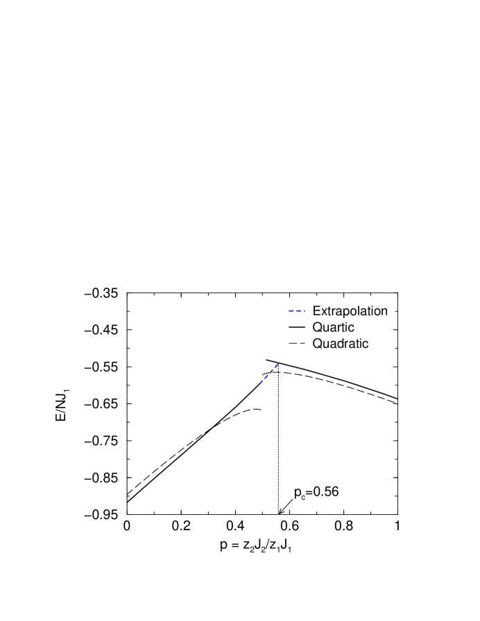
Figure 4: Zero temperature ground state energy per site, $E/NJ_{1}$, is plotted versus $p$ without (dashed lines) and with (solid lines) quartic corrections for both AF ($p<0.5$) and CAF ($p>0.5$) ordered phases. Spin wave theory becomes unstable close to the classical transition point ($p_{\rm class}\approx 0.5$) between the two phases. After extrapolation (shown by the dotted line), we find that the two energies meet at the quantum transition point, $p_{c}\approx 0.56$ or $J_{2}/J_{1}\approx 0.28$. This kink in the energy indicates a first-order quantum phase transition from the AF to CAF phase. Compared to the results without quartic corrections (long dashed lines) we find that the quartic corrections provide significant corrections to the ground state energy especially near the AF-CAF phase transition point.

In Fig. 4 we show the ground state energy per site, $E/NJ_{1}$, for the AF and the CAF phases with (solid line) and without (dashed line) quartic corrections as a function of the frustration parameter $p$. Classically $p_{\rm class}=0.5$ or $J_{2}/J_{1}=0.25$ is the critical point where a phase transition from the AF phase to one of the three CAF phases occur. With increase in frustration (as $p$ approaches 0.5 from both sides) we expect the GS energy to increase as the system goes from an energetically favored ordered state to a more disordered state. However, linear spin-wave theory calculation fails to capture this. Especially when $p$ is close to 0.5 we find a slight downward turn in energy. This has been reported in Ref. Kishi and Kubo, 1991. On the other hand, NLSWT calculation correctly produces the expected energy increase. At $p=0$ the calculated energy with the quartic corrections is slightly lower than the energy obtained without the quartic corrections. This small decrease from the LSWT calculation is due to the ground state energy correction, which is negative (as seen in Eq. 15 – these terms originate from the self-energy Hartree diagrams). As our spin-wave theory calculation becomes unstable in the regime $0.49<p<0.52$ we used a spline fit for the AF-phase energy data points and then extrapolated the line so that it intersects the CAF-phase energy line. The extrapolated curve is shown by dotted lines (color online) in the figure. After extrapolation, we find that the two energies meet at $p_{c}\approx 0.56$ or $J_{2}/J_{1}\approx 0.28$. The symmetries of the two phases are different: SO(3)/SO(2) for the AF phase and Z${}_{3}\times$SO(3)/SO(2) for the CAF phase. Diep (2004) Due to the different symmetries of the two phases the transition is of first order. This is confirmed by the kink in the energy at $p_{c}\approx 0.28$. Our obtained value from our self-consistent NLSWT calculations for the quantum critical point is $J_{2}/J_{1}\approx 0.28$. This is another major finding of our work.

Using the variational spin-wave theory the authors in Ref. Kishi and Kubo, 1991 obtained an upper bound of 0.27 for the ground state energy. However, their variational calculation slightly overestimates the value of GS energy. This is quite noticeable at $p=0$, where their energy value is higher than the LSWT prediction. We have found the $p=0$ energy value to be slightly less than the LSWT prediction. This is due to the quartic corrections explained earlier. The authors in Ref. Irkhin et al., 1992 used a modified spin-wave theory based on Dyson-Maleev representation of the spins to study this model. They numerically obtained the value of critical transition point to be $p_{c}=0.30$. The other known existing numerical work is by Diep et. al. Pinettes and Diep (1998) By extensive standard and histogram Monte-Carlo simulations, they obtained the transition point to be around 0.26. Our result is in excellent agreement with the results obtained from Monte-Carlo and variational spin-wave theory calculations (our $p_{c}$ differs by less than 3.5% from the variational spin-wave theory prediction).

V Conclusion

In this work we have investigated the zero temperature phases of a spin-$1/2$ Heisenberg frustrated AF on a SC lattice by considering the quartic $1/S$ corrections due to the spin-wave interactions. We have compared our results obtained from NLSWT calculations with the predictions from LSWT. It is known that LSWT predicts the existence of three phases: a two sublattice Néel phase for smaller values of the NNN exchange $J_{2}$, an intermediate paramagnetic phase, and a collinear phase for larger values of $J_{2}$. At zero temperature there are two quantum phase transitions - one from the AF-state to the disordered paramagnetic state and the other from the disordered state to one of the three collinear states. Both these transitions occur at the quantum critical point $p_{c}\approx 0.5$ or $J_{2}/J_{1}\approx 0.25$. We have found that quartic corrections significantly alter this phase diagram as intermediate paramagnetic phase disappears. We find the existence of two phases at zero temperature: a two sublattice AF phase for small $J_{2}$ and a collinear phase phase for large $J_{2}$. With the inclusion of quartic interactions the intermediate paramagnetic phase completely disappears. Due to the different symmetries of the two phases (AF and CAF) the transition between the two phases is of first order and we find that the critical point for transition to be 0.28. Our obtained result is in excellent agreement with existing numerical results from Monte Carlo simulations.

Appendix A Quartic terms for the AF phase

The quartic terms for the AF phase from the NN interactions involve $A-B$ interactions and for the NNN interactions involve $A-A$ and $B-B$ type interactions. Considering all these interactions the quartic Hamiltonian takes the form:

$$H^{(4)} = -J_{1}\sum_{\langle ij\rangle}\Big{[}a_{i}^{\dagger}a_{i}b^{\dagger}_{j}b_{j}+\frac{1}{4}\Big{(}a_{i}b^{\dagger}_{j}b_{j}b_{j}+a_{i}^{\dagger}a_{i}a_{i}b_{j}+h.c.\Big{)}\Big{]}$$ (26)

$$+ \frac{1}{2}J_{2}\sum_{[ij]}\Big{[}a^{\dagger}_{i}a_{i}a^{\dagger}_{j}a_{j}-\frac{1}{4}\Big{(}a_{i}a^{\dagger}_{j}a_{j}^{\dagger}a_{j}+a_{i}^{\dagger}a_{i}a_{i}a_{j}^{\dagger}+h.c.\Big{)}+a\leftrightarrow b\Big{]}.$$

In the harmonic approximation the following Hartree-Fock averages are non-zero for the SC-lattice Heisenberg antiferromagnet:

$$u_{1} = \langle a_{i}^{\dagger}a_{i}\rangle=\langle b_{i}^{\dagger}b_{i}\rangle=\frac{1}{2}\Big{[}\frac{2}{N}\sum_{\bf k}\frac{A^{(1)}_{{\bf k}}}{\omega^{(1)}_{{\bf k}}}-1\Big{]},$$ (27)

$$v_{1} = \langle a_{i}b_{j}\rangle=\langle a_{i}^{\dagger}b_{j}^{\dagger}\rangle=-\frac{1}{2}\Big{[}\frac{2}{N}\sum_{\bf k}\frac{\gamma_{1{\bf k}}B^{(1)}_{{\bf k}}}{\omega^{(1)}_{{\bf k}}}\Big{]},$$ (28)

$$w_{1} = \langle a_{i}^{\dagger}a_{j}\rangle=\langle b_{i}^{\dagger}b_{j}\rangle=\frac{1}{2}\Big{[}\frac{2}{N}\sum_{\bf k}\frac{\gamma_{2{\bf k}}A^{(1)}_{{\bf k}}}{\omega^{(1)}_{{\bf k}}}\Big{]},$$ (29)

where $\omega^{(1)}_{{\bf k}}=\sqrt{\Big{(}A^{(1)}_{{\bf k}}\Big{)}^{2}-\Big{(}B^{(1)}_{{\bf k}}\Big{)}^{2}}.$

Appendix B Quartic terms for the CAF phase

The quartic terms for the collinear phase from the NN interactions involve interactions between the sublattices $B-C$ and $A-D$ along the $x$ axis, $A-C$ and $B-D$ along the $y$ axis, and $A-B$ and $C-D$ along the $z$ axis. For the NNN interactions spin-spin interactions are between sublattices $A-B$ and $C-D$ (in the $xy$-plane), $A-C$ and $B-D$ (in the $xz$-plane), and $A-D$ and $B-C$ (in the $yz$-plane) as shown in Fig. 1(b). Adding all the contributions together yield

$$H^{(4)} = -J_{1}\sum_{\langle ij_{x}\rangle}\Big{[}a_{i}^{\dagger}a_{i}b^{\dagger}_{j_{x}}b_{j_{x}}+\frac{1}{4}\Big{(}a_{i}b^{\dagger}_{j_{x}}b_{j_{x}}b_{j_{x}}+a_{i}^{\dagger}a_{i}a_{i}b_{j_{x}}+h.c.\Big{)}\Big{]}$$ (30)

$$- J_{1}\sum_{\langle ij_{y}\rangle}\Big{[}a_{i}^{\dagger}a_{i}b^{\dagger}_{j_{y}}b_{j_{y}}+\frac{1}{4}\Big{(}a_{i}b^{\dagger}_{j_{y}}b_{j_{y}}b_{j_{y}}+a_{i}^{\dagger}a_{i}a_{i}b_{j_{y}}+h.c.\Big{)}\Big{]}$$

$$+ \frac{1}{2}J_{1}\sum_{\langle ij_{z}\rangle}\Big{[}a^{\dagger}_{i}a_{i}a^{\dagger}_{j_{z}}a_{j_{z}}-\frac{1}{4}\Big{(}a_{i}a^{\dagger}_{j_{z}}a_{j_{z}}^{\dagger}a_{j_{z}}+a_{i}^{\dagger}a_{i}a_{i}a_{j_{z}}^{\dagger}+h.c.\Big{)}+a\leftrightarrow b\Big{]}$$

$$+ \frac{1}{2}J_{2}\sum_{\langle ij_{xy}\rangle}\Big{[}a^{\dagger}_{i}a_{i}a^{\dagger}_{j_{xy}}a_{j_{xy}}-\frac{1}{4}\Big{(}a_{i}a^{\dagger}_{j_{xy}}a_{j_{xy}}^{\dagger}a_{j_{xy}}+a_{i}^{\dagger}a_{i}a_{i}a_{j_{xy}}^{\dagger}+h.c.\Big{)}+a\leftrightarrow b\Big{]}$$

$$- J_{2}\sum_{\langle ij_{yz}\rangle}\Big{[}a_{i}^{\dagger}a_{i}b^{\dagger}_{j_{yz}}b_{j_{yz}}+\frac{1}{4}\Big{(}a_{i}b^{\dagger}_{j_{yz}}b_{j_{yz}}b_{j_{yz}}+a_{i}^{\dagger}a_{i}a_{i}b_{j_{yz}}+h.c.\Big{)}\Big{]}$$

$$- J_{2}\sum_{\langle ij_{xz}\rangle}\Big{[}a_{i}^{\dagger}a_{i}b^{\dagger}_{j_{xz}}b_{j_{xz}}+\frac{1}{4}\Big{(}a_{i}b^{\dagger}_{j_{xz}}b_{j_{xz}}b_{j_{xz}}+a_{i}^{\dagger}a_{i}a_{i}b_{j_{xz}}+h.c.\Big{)}\Big{]}.$$

Above $j_{x},j_{y},j_{z}$ are NN lattice sites along $x,y,z$ axes and $j_{xy},j_{yz},j_{xz}$ connects one lattice site with a NNN corner lattice sites on the $xy,yz,xz$ planes. The different coefficients that originate from Hartree-Fock decoupling process are

$${\overline{u}} = \langle a_{i}^{\dagger}a_{i}\rangle=\langle b_{i}^{\dagger}b_{i}\rangle=\frac{1}{2}\Big{[}\frac{2}{N}\sum_{\bf k}\frac{A^{(2)}_{{\bf k}}}{\omega^{(2)}_{{\bf k}}}-1\Big{]},$$ (31)

$${\overline{v}_{1x}} = \langle a_{i}b_{j_{x}}\rangle=\langle a_{i}^{\dagger}b_{j_{x}}^{\dagger}\rangle=-\frac{1}{6}\Big{[}\frac{2}{N}\sum_{\bf k}\frac{\cos k_{x}B^{(2)}_{{\bf k}}}{\omega^{(2)}_{{\bf k}}}\Big{]},$$ (32)

$${\overline{v}_{1y}} = \langle a_{i}b_{j_{y}}\rangle=\langle a_{i}^{\dagger}b_{j_{y}}^{\dagger}\rangle=-\frac{1}{6}\Big{[}\frac{2}{N}\sum_{\bf k}\frac{\cos k_{y}B^{(2)}_{{\bf k}}}{\omega^{(2)}_{{\bf k}}}\Big{]},$$ (33)

$${\overline{v}_{2yz}} = \langle a_{i}b_{j_{yz}}\rangle=\langle a_{i}^{\dagger}b_{j_{yz}}^{\dagger}\rangle=-\frac{1}{6}\Big{[}\frac{2}{N}\sum_{\bf k}\frac{\cos k_{y}\cos k_{z}B^{(2)}_{{\bf k}}}{\omega^{(2)}_{{\bf k}}}\Big{]},$$ (34)

$${\overline{v}_{2xz}} = \langle a_{i}b_{j_{xz}}\rangle=\langle a_{i}^{\dagger}b_{j_{xz}}^{\dagger}\rangle=-\frac{1}{6}\Big{[}\frac{2}{N}\sum_{\bf k}\frac{\cos k_{x}\cos k_{z}B^{(2)}_{{\bf k}}}{\omega^{(2)}_{{\bf k}}}\Big{]},$$ (35)

$${\overline{w}_{z}} = \langle a_{i}^{\dagger}a_{j_{z}}\rangle=\langle b_{i}^{\dagger}b_{j_{z}}\rangle=\frac{1}{6}\Big{[}\frac{2}{N}\sum_{\bf k}\frac{\cos k_{z}A^{(2)}_{{\bf k}}}{\omega^{(2)}_{{\bf k}}}\Big{]},$$ (36)

$${\overline{w}_{1}} = \langle a_{i}^{\dagger}a_{j_{xy}}\rangle=\langle b_{i}^{\dagger}b_{j_{xy}}\rangle=\frac{1}{6}\Big{[}\frac{2}{N}\sum_{\bf k}\frac{\cos k_{x}\cos k_{y}A^{(2)}_{{\bf k}}}{\omega^{(2)}_{{\bf k}}}\Big{]},$$ (37)

where $\omega^{(2)}_{{\bf k}}=\sqrt{\Big{(}A^{(2)}_{{\bf k}}\Big{)}^{2}-\Big{(}B^{(2)}_{{\bf k}}\Big{)}^{2}}.$ By symmetry ${\overline{v}_{1x}}={\overline{v}_{1y}}={\overline{v}_{1}}$ and ${\overline{v}_{2yz}}={\overline{v}_{2xz}}={\overline{v}_{2}}$.

(a)  AF phase

(b)  CAF phase

Figure 1: AF and collinear antiferromagnetic (CAF) ordered phases of the SC lattice. In the AF phase all $A$-sublattice spins point in the direction of an arbitrary unit vector while $B$-sublattice spins point in the opposite direction. For the CAF phase the spin configurations (lines of spins up and down) of the four sublattices A,B,C, and D are shown in the Figure. There are two other equivalent configurations with lines along the two other directions of the cubic lattice.

Figure 2: Self-consistent results for the different parameters, $u_{1},v_{1},w_{1}$ (for the AF-phase) and ${\overline{u}_{1}},{\overline{v}_{1}},{\overline{v}_{2}},{\overline{w}_{1}},{\overline{w}_{z}}$ (for the CAF phase) are plotted with the frustration parameter $p=z_{2}J_{2}/z_{1}J_{1}$ (for the SC lattice $z_{1}=6$ and $z_{2}=12$). These coefficients vary significantly with $p$, which shows that the quartic interaction terms play a significant role in determining the different phases of our model.

Figure 3: Average sublattice magnetization, $\langle S_{\alpha}\rangle$, is plotted with the frustration parameter $p$ for AF and one of the three CAF phases with (solid lines) and without (dashed lines) quartic corrections. At zero temperature without the quartic $1/S$ corrections (linear spin-wave theory) $\langle S_{\alpha}\rangle\rightarrow 0$ at $p_{c1}\approx 0.48$ indicating a phase transition from the AF-ordered state to the disordered paramagnetic state. At $p_{c2}=0.50$ there is a second phase transition from the collinear state to the disordered state for $T=0$. Non-linear spin wave theory provides significant corrections to this phase diagram. With the quartic $1/S$ corrections the disordered PM region disappears completely and we only obtain two phases: AF and CAF. There is no existence of any disordered state as predicted by the linear spin-wave theory (quadratic corrections). For both the phases the quartic corrections to the Hamiltonian enhance the magnetic order.

References

- Diep (2004) H. T. Diep, Frustrated Spin Systems (World Scientific, Singapore, 2004), 1st ed.
- Sachdev (2001) S. Sachdev, Quantum Phase Transitions (Cambridge University Press, Cambridge, UK, 2001), 1st ed.
- (3) S. Sachdev, eprint cond-mat.str-el/0901.4103.
- Rastelli et al. (1979) E. Rastelli, A. Tassi, and L. Reatto, Physica 97B, 1 (1979).
- Reatto and Tassi (1985) E. R. L. Reatto and A. Tassi, J. Phys. C: Solid State Phys. 18, 353 (1985).
- Barabanov and Starykh (1990) A. F. Barabanov and O. A. Starykh, JETP Letts. 51, 311 (1990).
- Sachdev (1992a) S. Sachdev, Phys. Rev. B 45, 12 377 (1992a).
- Dotsenko and Sushkov (1994) A. V. Dotsenko and O. Sushkov, Phys. Rev. B 50, 13 821 (1994).
- Chubukov (1992a) A. Chubukov, Phys. Rev. Lett. 69, 832 (1992a).
- Gelfand et al. (1989) M. P. Gelfand, R. R. P. Singh, and D. A. Huse, Phys. Rev. B 40, 10801 (1989).
- Sushkov et al. (2001) O. P. Sushkov, J. Oitmaa, and Z. Weihong, Phys. Rev. B 63, 104420 (2001).
- Weihong et al. (1999) Z. Weihong, R. H. McKenzie, and R. R. P. Singh, Phys. Rev. B 59, 14 367 (1999).
- Singh et al. (1999) R. R. P. Singh, Z. Weihong, C. J. Hammer, and J. Oitmaa, Phys. Rev. B 60, 7278 (1999).
- Irkhin et al. (1992) V. Y. Irkhin, A. A. Katanin, and M. I. Katsnelson, J. Phys.: Condens. Matter 4, 5227 (1992).
- Canals and Lacroix (1998) B. Canals and C. Lacroix, Phys. Rev. Lett. 80, 2933 (1998).
- Fak et al. (2008) B. Fak, F. C. Coomer, A. Harrison, D. Visser, and M. E. Zhitomirsky, EPL. 81, 17006 (2008).
- Sachdev (1992b) S. Sachdev, Phys. Rev. B 45, 12 377 (1992b).
- Chubukov (1992b) A. Chubukov, Phys. Rev. Lett. 69, 832 (1992b).
- Harris et al. (1992) A. B. Harris, C. Kallin, and A. J. Berlinsky, Phys. Rev. B 45, 2899 (1992).
- Oitmaa and Zheng (2004) J. Oitmaa and W. Zheng, Phys. Rev. B 69, 064416 (2004).
- Schmidt et al. (2002) R. Schmidt, J. Schulenburg, and J. Richter, Phys. Rev. B 66, 224406 (2002).
- Majumdar and Datta (2009) K. Majumdar and T. Datta, J. Phys.: Condes. Matter 21, 406004 (2009).
- Azaria (1986) P. Azaria, J. Phys. C: Solid State Phys. 19, 2773 (1986).
- Derrida et al. (1979) B. Derrida, Y. Pomeau, G. Toulouse, and J. Vannimenus, J. Physique 40, 617 (1979).
- Derrida et al. (1980) B. Derrida, Y. Pomeau, G. Toulouse, and J. Vannimenus, J. Physique 41, 213 (1980).
- Lallemand et al. (1985) P. Lallemand, H. T. Diep, A. Ghazali, and G. Toulouse, J. Phys. Lett. 46, L (1985).
- Karchev (2008) N. Karchev, J. Phys.: Condens. Matter 20, 325219 (2008).
- Karchev (2009) N. Karchev, J. Phys.: Condens. Matter 21, 216003 (2009).
- Banavar et al. (1979) J. R. Banavar, D. Jasnow, and D. P. Landau, Phys. Rev. B 20, 3820 (1979).
- Oguchi et al. (1985) T. Oguchi, H. Nishimori, and Y. Taguchi, J. Phys. Soc. Japan 54, 4494 (1985).
- Ignatenko et al. (2008) A. N. Ignatenko, A. A. Katanin, and V. Y. Irkhin, JETP Letts. 87, 1 (2008).
- Diep and Kawamura (1989) H. T. Diep and H. Kawamura, Phys. Rev. B 40, 7019 (1989).
- Ader (2002) J. P. Ader, Phys. Rev. B 66, 174414 (2002).
- Villain (1959) J. Villain, J. Phys. Chem. Solids 11, 303 (1959).
- Villain (1977) J. Villain, J. Phys. C: Solid State Phys. 10, 1717 (1977).
- Pinettes and Diep (1998) C. Pinettes and H. T. Diep, J. Appl. Phys. 83, 6317 (1998).
- Diep et al. (1985) H. T. Diep, A. Ghazali, and P. Lallemand, J. Phys. C: Solid State Phys. 18, 5881 (1985).
- Kishi and Kubo (1991) T. Kishi and K. Kubo, Phys. Rev. B 43, 10844 (1991).
- Viana et al. (2008) J. R. Viana, J. R. de Sousa, and M. Continentino, Phys. Rev. B 77, 172412 (2008).
- (40) Note that defined here differs by a factor with the definition of in the introduction.
- Shender (1982) E. F. Shender, Sov. Phys. JETP 56, 178 (1982).
- Henley (1989) C. L. Henley, Phys. Rev. Lett. 62, 2056 (1989).
- Kubo and Kishi (1991) K. Kubo and T. Kishi, J. Phys. Soc. Japan 60, 567 (1991).