SCATTERING AND DUALITY IN THE 2 DIMENSIONAL $OSP(2|2)$ GROSS NEVEU AND SIGMA MODELS

Abstract

We write the thermodynamic Bethe ansatz for the massive $OSp(2|2)$ Gross Neveu and sigma models. We find evidence that the GN S matrix proposed by Bassi and Leclair [12] is the correct one. We determine features of the sigma model S matrix, which seem highly unconventional; we conjecture in particular a relation between this sigma model and the complex sine-Gordon model at a particular value of the coupling. We uncover an intriguing duality between the $OSp(2|2)$ GN (resp. sigma) model on the one hand, and the $SO(4)$ sigma (resp. GN model) on the other, somewhat generalizing to the massive case recent results on $OSp(4|2)$. Finally, we write the TBA for the (SUSY version of the) flow into the random bond Ising model proposed by Cabra et al. [39], and conclude that their S matrix cannot be correct.

1 Introduction

The study of $1+1$ quantum field theories with supergroup symmetry is a lively and difficult topic, central to several key areas of modern physics, in particular the solution of critical points in non interacting disordered systems, and the AdS/CFT conjecture.

It is natural to try to make progress by focussing on integrable theories. By analogy with the ordinary case, one can expect the simplest possible situations to be encountered [1] in the $OSp(n|2m)$ Gross Neveu and sigma models. Yet, apart from the special case of $OSp(1|2)$ which behaves much like an ordinary group [2, 3], only little progress has been accomplished, largely for what seems to be technical reasons. Another exception is the case of $OSp(4|2)$, where, among other fascinating properties [4], a striking duality between the GN and sigma model was uncovered [5, 6].

The case of $OSp(2|2)$ is particularly tentalizing, since it is the ‘simplest’ after $OSp(1|2)$, and plays a major role in disordered systems. Yet, even here, significant progress has only occurred up to now in the critical case, where WZW theories have been solved [7], and their relation with spin chains understood [8, 9]. Our main goal in this paper is to understand the massive theories: the GN and $OSp(2/2)/OSp(1/2)$ ‘supersphere’ sigma models.

To proceed, we recall some general features in the ordinary $O(N)$ bosonic case. The actions are well known [10]. The S matrices involve generically particles in the  (vector) representation. Introducing the useful graphical representation of invariant tensors

Figure 1: Graphical representation of the invariant tensors appearing in the $S$ matrix.

there are generically two known models whose scattering matrix for the vector representation has the form in figure 1, with none of the $\sigma_{i}$’s vanishing. They are given by

$$\sigma_{1} = -{2i\pi\over(N-2)(i\pi-\theta)}~{}\sigma_{2}$$

$$\sigma_{3} = -{2i\pi\over(N-2)\theta}~{}\sigma_{2}$$ (1)

with two possible choices for $\sigma_{2}$:

$$\sigma_{2}^{\pm}(\theta)={\Gamma\left(1-{\theta\over 2i\pi}\right)\over\Gamma\left({\theta\over 2i\pi}\right)}{\Gamma\left({1\over 2}+{\theta\over 2i\pi}\right)\over\Gamma\left({1\over 2}-{\theta\over 2i\pi}\right)}{\Gamma\left(\pm{1\over N-2}+{\theta\over 2i\pi}\right)\over\Gamma\left(1\pm{1\over N-2}-{\theta\over 2i\pi}\right)}{\Gamma\left({1\over 2}\pm{1\over N-2}-{\theta\over 2i\pi}\right)\over\Gamma\left({1\over 2}\pm{1\over N-2}+{\theta\over 2i\pi}\right)}$$ (2)

The factor $\sigma_{2}^{+}$ does not have poles in the physical strip for $N\geq 0$, and the corresponding S matrix for $N\geq 3$ is believed to describe the $O(N)/O(N-1)$ sphere ($S^{N-1}$) sigma model. The factor $\sigma_{2}^{-}$ does not have poles in the physical strip for $N\leq 4$. For $N>4$, it describes the scattering of vector particles in $O(N)$ Gross Neveu model. Recall that for $N=3,4$ the vector particles in the GN model are unstable and disappear from the spectrum, that contains only kinks. Some of these features are illustrated for convenience in figure 2.

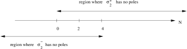
Figure 2: Pole structure of $\sigma_{2}$ as a function of $N$. Except for a finite region at small $N$, the generic S matrix with $\sigma_{2}^{+}$ describes the sigma model and the one with $\sigma_{2}^{-}$ the GN model.

Note that at vanishing rapidity, the scattering matrix reduces to $\check{S}(\theta=0)=\mp I$. This is in agreement with the fundamental particles being bosons in the sigma model , and fermions in the Gross Neveu model [11].

It was argued in [1] that for $N$ negative and $|N|$ large enough, a similar S matrix - where now the invariant tensors have to be interpreted within $OSp(m|2n)$ representation theory - still describes the GN and sigma models provided one sets $N=m-2n$. The detailed calculations performed in [1] show that one the roles of the two models remains the same, that is, $\sigma_{+}$ still corresponds to the sigma model and $\sigma_{-}$ to the GN model.

This has several interesting consequences. One is, that the GN model exhibits bound states while the sigma model does not, for $N$ large, ie $m>>2n$; meanwhile, the sigma model does then exhibit bound states - and the GN none - for $-N$ large, ie $m<<2n$. Where exactly these behaviours may be modified at small $N$ is a partly open question. We emphasize that, although the S matrices are presumably known in the generic case, no systematic check has been performed, as writing the TBA has proven, up to now, too cumbersome.

A crucial observation based again on [1] and also [3] is that the massive continuum limit of the integrable lattice model based on the fundamental of $OSp(m|2n)$ always exhibits bound states. Therefore it necessarily corresponds to the GN model for $N>2$ and the sigma model for $N<2$ (including $N$ negative of course). The case $N=2$ being at the border suggests that the sigma and the GN model are then dual of each of other. This is of course well known for $O(2)$, and has recently been established, for a certain choice of boundary conditions, in the orthosymplectic case [5], [6]. Note that the S matrices for the sigma and GN model at $N=2$ also coincide. They describe a special point on the critical lines of either (dual) model.

The case $N=0$ ($OSp(2n|2n)$) is the next case that seems really worth studying. Indeed, right at $N=0$, $\sigma_{2}^{+}=\sigma_{2}^{-}$ (and the foregoing S matrix coincides with the one in [12]), while it is clear that the GN and sigma models are different (see below for detailed actions etc). Something is thus missing from the general picture. On the other hand, the TBA should not be too complicated. It is particularly tractable for a special choice of Dynkin diagram first studied in [13].

The $OSp(2|2)$ has also the potential to exhibit interesting duality properties. To see this, consider another - a priori more anecdotical - remark about the beta functions of the sigma and GN models . In an expansion in the coupling constant the first two non trivial coefficients obey:

$${\beta_{2}\over\beta_{1}^{2}}={1\over N-2}\hbox{ sigma model}$$

$${\beta_{2}\over\beta_{1}^{2}}=-{1\over N-2}\hbox{ GN model}$$ (3)

These two results are exchanged under $N-2\rightarrow 2-N$. This suggests there might be some relationship between the $O(N)$ GN model and $O(4-N)$ sigma models, where an $OSp$ supergroup has to be used whenever necessary.

Of course, these two models cannot be related in general: among other things, their UV central charges don’t match for arbitrary N. Nevertheless, as observed in [1], some of the S matrix elements match exactly under this transformation. One has indeed,

$$\left[\sigma_{2}^{+}-\sigma_{3}^{+}\right](N)=\left[\sigma_{2}^{-}+\sigma_{3}^{-}\right](4-N)$$ (4)

This implies that, at zero temperature and with the proper applied field $h$ , the ground state energies of the $O(N)$ GN model and the one of the $O(4-N)$ sigma model do indeed coincide as functions of $h/M$ (and in particular, their zero field energies - the regularized version of the ground state energy as a function of the mass $M$ - coincide).

Now, if we take the $OSp(2|2)$ GN ($N=0$) model we have $c=0,c_{\hbox{eff}}=3$ , while for the $SO(4)$ sigma model we have $c=3$ (no fermions in this case). So some identificatiom might be possible. Similarly, if we take the $OSP(2|2)$ sigma model we have $c=-1,c_{\hbox{eff}}=2$ while for the $SO(4)$ GN model, which is a sum of two independent sine Gordon models at the marginal point, $c=2$, again allowing a potential identification. This pattern generalizes immediately to the case of $OSp(2n|2n)$ and $OSp(2n|2n-4)$:

$$OSp(2n|2n)\hbox{ GN model }:c=0,c_{\hbox{eff}}=3n$$

$$OSp(2n+2|2n-2)\hbox{Sigma model }:c=3,~{}c_{\hbox{eff}}=3n$$

$$OSp(2n|2n)\hbox{Sigma model}:c=-1,~{}c_{\hbox{eff}}=3n-1$$

$$OSp(2n+2|2n-2)\hbox{GN model }:c=2,~{}c_{\hbox{eff}}=3n-1$$ (5)

One of the questions we will investigate in this paper is the potential duality between these two families of models for the simplest case $n=1$.

Our strategy will be based on non perturbative calculations of the free energies at finite temperature of all models using an S matrix and thermodynamic Bethe ansatz approach.

Because of the common underlying $osp(2|2)\equiv sl(2|1)$ symmetry, the different Bethe ansätze involved have a common structure of roots and basic equations, which coincide with those for the integrable spin chains. We thus discuss these common features first.

2 Solving the monodromy problem: the Bethe ansatz for integrable SL(2$|$1) vertex models and spin chains

2.1 The Bethe equations in the fermionic grading

We start with the Bethe equations for the $sl(2/1)$ spin chain built out of alternating $3$ and $\bar{3}$ representations, that is the Hilbert space is $3^{\otimes L}\otimes\bar{3}^{\otimes L}$. There are different Bethe ansätze available, and as often, chosing the right one can be a big help. We take the Bethe ansatz based on a choice of purely fermionic simple roots [15] for the $sl(2|1)$ algebra.

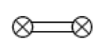
Figure 3: Dynkin diagram leading to our Bethe equations

Recall that the Bethe equations read then [13, 8]

$$\left({u_{j}+i\over u_{j}-i}\right)^{L}=\prod_{\beta=1}^{M}{u_{j}-\gamma_{\beta}+i\over u_{j}-\gamma_{\beta}-i},~{}~{}~{}j=1,\ldots,N$$

$$\left({\gamma_{\alpha}+i\over\gamma_{\alpha}-i}\right)^{L}=\prod_{k=1}^{N}{\gamma_{\alpha}-u_{k}+i\over\gamma_{\alpha}-u_{k}-i},~{}~{}~{}\alpha=1,\ldots,M$$ (6)

with the quantum numbers $B={N-M\over 2}$and $J^{3}=L-{M+N\over 2}$. The corresponding energy, for the regime of interest here, is is

$$E\propto-\left(\sum_{k=1}^{N}{1\over u_{k}^{2}+1}+\sum_{\beta=1}^{M}{1\over\gamma_{\beta}^{2}+1}\right)$$ (7)

A crucial observation [8] which allows one to draw some conclusions quickly is that this system of equations admits a particular solution made of sets such that $N=M$ and $u_{j}=\gamma_{\beta}$. The roots then have to satisfy

$$\left({u_{j}+i\over u_{j}-i}\right)^{L}=\prod_{k=1}^{n}{u_{j}-u_{k}+i\over u_{j}-u_{k}-i}$$ (8)

a system of equations that is identical with the Bethe equations for the spin 1 antiferromagnetic XXX chain (we often refer to the latter simply as XXX, or the Takhtajan-Babujian [16], chain). Notice however that the dynamics is such that the gaps in our system will be twice the gaps in the latter chain: sound velocities have to be adjusted appropriately. Often, we will see that our results are in some sense a ‘doubling’ of those for this XXX chain.

The argument extends to a chain with alternating fully symmetric and antisymmetric representations, represented by Young diagrams with $p$ boxes . The bare Bethe ansatz equations then look exactly as (6) but in the left hand side, the factors $i$ are replaced by $pi$, and similarly for the energy (7) the $1$ in the denominator is replaced by $p^{2}$. This time, the symmetric sector $N=M$, $u_{j}=\gamma_{\beta}$, is related with the XXX chain of (integer) spin $p$.

The argument also works for the model in the fundamental representation of $osp(2/2)$. In that case indeed, the bare Bethe ansatz equations and the energy still read as (6,7) but with the factor $i$ replaced by $i/2$ (ie, formally, $p=1/2$ in the foregoing discussion):

$$\left({u_{j}+i/2\over u_{j}-i/2}\right)^{L} = \prod_{\beta=1}^{M}{u_{j}-\gamma_{\beta}+i\over u_{j}-\gamma_{\beta}-i},~{}~{}~{}j=1,\ldots,N$$

$$\left({\gamma_{\alpha}+i/2\over\gamma_{\alpha}-i/2}\right)^{L} = \prod_{k=1}^{N}{\gamma_{\alpha}-u_{k}+i\over\gamma_{\alpha}-u_{k}-i},~{}~{}~{}\alpha=1,\ldots,M,~{}~{}~{}\hbox{fundamental of $OSp(2|2)$}$$ (9)

This time the symmetric sector is related with the spin $1/2$ chain. Note that, while the equations (6) hold for a system made of $L$ representations $3$ and $L$ representations $\bar{3}$, when it comes to the fundamental of $osp(2/2)$, (9) holds for $L$ representations $4$.

2.2 The solutions for large chains

Like for the XXX chain, the types of solutions of the Bethe equations do not depend on the source terms, and can be discussed in full generality . The standard way to classify the solutions is to consider configurations of spectral parameters that sit on poles of the bare scattering kernels (the right-hand-sides in (6,9)). A simple calculation yields the following types of “strings”

• “Reals”:

  unpaired, purely real spectral parameters $u_{j}$ and $\gamma_{\beta}$.

• “Wide strings”:

  “type-I”: composites containing $n-1$ $\gamma$’s and $n$ $u$’s ($n>1$)

  $$u_{\alpha,k}^{(n,n-1)} = u_{\alpha}^{(n,n-1)}+i\left(n+1-2k\right),\quad k=1\ldots n$$

  $$\gamma_{\alpha,j}^{(n,n-1)} = u_{\alpha}^{(n,n-1)}+i\left(n-2j\right),\quad j=1\ldots n-1\ ,\quad u_{\alpha}^{(n,n-1)}\in{\rm I\!R}$$ (10)

  “type-II”: composites containing $n$ $\gamma$’s and $n-1$ $u$’s ($n>1$)

  $$\gamma_{\alpha,k}^{(n,n-1)} = u_{\alpha}^{(n,n-1)}+i\left(n+1-2k\right),\quad k=1\ldots n$$

  $$u_{\alpha,j}^{(n,n-1)} = u_{\alpha}^{(n,n-1)}+i\left(n-2j\right),\quad j=1\ldots n-1\ ,\quad u_{\alpha}^{(n,n-1)}\in{\rm I\!R}$$ (11)

  

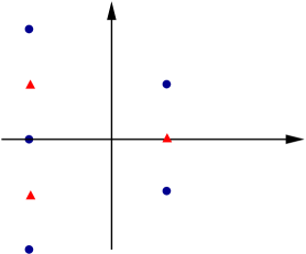
  Figure 4: Wide strings of lengths three and two respectively. The circles/triangles denote the positions of the $u$’s/$\gamma$’s involved in the string.

• “Strange strings”:

  composites containing $n$ $\gamma$’s and $n$ $u$’s ($n\geq 1$)

  $$u_{\alpha,k}^{(n,+)} = u_{\alpha}^{(n)}+i(n+1-2k-\frac{1}{2}),\quad k=1,\ldots,n\ ,$$

  $$\gamma_{\alpha,k}^{(n,+)} = u_{\alpha}^{(n)}-i(n+1-2k-\frac{1}{2})\ ,\quad u_{\alpha}\in{\rm I\!R},$$ (12)

  or

  $$u_{\alpha,k}^{(n,-)} = u_{\alpha}^{(n)}-i(n+1-2k-\frac{1}{2}),\quad k=1,\ldots,n\ ,$$

  $$\gamma_{\alpha,k}^{(n,-)} = u_{\alpha}^{(n)}+i(n+1-2k-\frac{1}{2})\ ,\quad u_{\alpha}\in{\rm I\!R},$$ (13)

  It is fundamental to observe that solutions of this type are fundamentally different from the usual string solutions in that the set of roots on one level of the Bethe equations is not invariant under complex conjugation. The other solutions discussed above (reals and wide strings) are invariant under this operation. This is similar to what was found recently for the anisotropic $sl(3)$ chain related with the complex $SU(3)$ Toda theory in the continuum limit [17]. Of course this non invariance reflects the non hermitian nature of the superalgebra hamiltonian: it casts doubts on analyzing the ‘thermodynamics’ of the system, for instance, but we shall see that naive calculations seem to give the correct results anyway. Note that although “strange strings” are not invariant under complex conjugation, the corresponding energy (7)is still real because it depends symmetrically on the $u$ and $\gamma$ parameters.

  

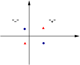
  Figure 5: The two types of $n=1$ strange strings

  

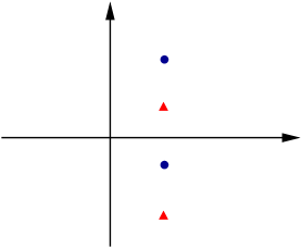
  Figure 6: A strange string with $n=2$.

• “Narrow strings”:

  composites containing $n$ $\gamma$’s and $n$ $u$’s ($n>1$)

  $$u_{\alpha,k}^{(n,n)} = u_{\alpha}^{(n,n)}+\frac{i}{2}\left(n+1-2k\right),\quad k=1\ldots n$$

  $$\gamma_{\alpha,j}^{(n,n)} = u_{\alpha}^{(n,n)}+\frac{i}{2}\left(n+1-2j\right),\quad j=1\ldots n\ ,\quad u_{\alpha}^{(n,n)}\in{\rm I\!R}$$ (14)

  Narrow strings may be thought of as special cases of strange strings or wide strings in the following sense.

  • Combining a “+”-strange string of length $n$ and centre $u^{(n)}$ with a a “-”-strange string of length $n$ and centre $u^{(n)}$ we obtain a narrow string of even length $2n$. This is shown for $n=1$ in Fig.7(a).

  • Combining a type-1 wide string of length n and centre $u^{(n,n-1)}$ with a type-2 wide string of length n and centre $u^{(n,n-1)}$ we obtain a narrow string of length $2n-1$. This is shown for the case $n=2$ in Fig. 8(b).

  

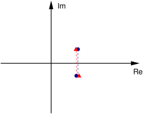
  Figure 7: Combining a pair of “+” and “-” strange strings of length $1$ gives a narrow string of length $2$;

  

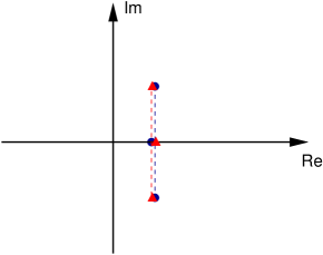
  Figure 8: Combining a type-1 wide string on length 2 with a type-2 wide string of length 2 gives a narrow string of length $3$;

  It is clear from our discussion that narrow strings are not “fundamental” but are merely degenerate cases of strange string solutions of the Bethe ansatz equations.

3 TBA for the $3,\bar{3}$ and the $4$ (fundamental of OSp(2$|$2)) spin chains

We now derive the TBA equations for the gapless spin chains to check (some aspects of) the completeness of our classification of solutions, and prepare subsequent discussion.

To start we derive equations for the densities of these various solutions in the limit of large systems. This is done as usual by considering that the various roots in the complexes are slightly off, and eliminating the corresponding small shifts through the Bethe equations, resulting in ‘higher’ Bethe equations. After taking the logarithm and naively differentiating, we get a system which we write symbolically as

$$\rho_{i}+\rho_{i}^{h}=s_{i}+\sum_{j}\Phi_{ij}\star\rho_{j}$$ (15)

(note we have included a $2\pi$ into the definition of the source and kernels). We introduce the fundamental objects

$$\alpha_{t}(u)={u+it/2\over u-it/2}$$ (16)

and the Fourier transformation

$$\hat{f}(x)=\int due^{iux}f(u),~{}~{}~{}f(u)={1\over 2\pi}\int dxe^{-iux}f(x)$$ (17)

We also set

$$a_{t}(u)={i\over 2\pi}{d\over du}\ln[\alpha_{t}(u)]={1\over 2\pi}{t\over u^{2}+t^{2}/4}$$ (18)

so that $\hat{a}_{t}(x)=e^{-t|x|/2}$. Let us now give explicitly the terms in (15).

The source terms (that is, the terms in the left hand side of the Bethe equations) in the case of alternating $3$ and $\bar{3}$ (6) for $n$ wide strings of type I or type II are of the form $\alpha_{2n-2}\alpha_{2n}$ which gives, after taking the log and differentiating, source terms of the form

$$\hat{s}_{I,n}^{w}=\hat{s}_{II,n}^{w}=a_{2n}+a_{2n-2},~{}~{}~{}n\geq 1$$ (19)

with the convention that $a_{0}=0$, and that wide strings with $n=1$ are just real strings. Similarly, the source terms for $n$ strange strings of type I or type II are still complex numbers of modulus one, $e_{2n-1}e_{2n+1}$, and give after taking the logarithm and differentiating, real source terms of the form

$$\hat{s}_{I,n}^{s}=\hat{s}_{II,n}^{s}=a_{2n-1}+a_{2n+1},~{}~{}~{}n\geq 1$$ (20)

The kernel of interaction between $n$ wide strings of type I and $p$ wide strings of type I reads

$$\alpha_{2p-2n}\alpha^{2}_{2p-2n+4}\ldots\alpha^{2}_{2p+2n-4}$$ (21)

while the interaction between $n$ wide strings of type I and $p$ wide strings of type II is instead

$$\alpha_{2p+2n-2}\alpha^{2}_{2p-2n-6}\ldots\alpha^{2}_{2p-2n+2}$$ (22)

and there is a symmetry between type I and type II strings.

Taking the logarithm and differentiating gives the Fourier transforms of the functions $\Phi$ in (see 15)

$$\hat{\Phi}_{I,n;I,p}^{w;w}=\hat{\Phi}_{I,p;I,n}^{w;w}=-2{\sinh nx\over\sinh x}e^{-(p-1)|x|}+e^{-(p-n)|x|}+\delta_{np},~{}~{}~{}p\geq n$$

$$\hat{\Phi}_{I,n;II,p}^{w,w}=\hat{\Phi}_{II,p;I,n}^{w,w}=-2{\sinh nx\over\sinh x}e^{-|p|x}-e^{-(p+n-1)|x|},~{}~{}~{}p\geq n$$ (23)

Note that

$$\hat{\Phi}_{I,n;I,p}^{w;w}+\hat{\Phi}_{I,n;II,p}^{w,w}=-A_{2n-1,2p-1}+\delta_{n,p}$$ (24)

where

$$A_{r,s}\equiv 2{\cosh x/2\over\sinh x/2}\sinh[rx/2]e^{-s|x|/2},~{}~{}~{}s\geq r,~{}~{}~{}A_{r,s}=A_{s,r}$$ (25)

and $-A_{rs}+\delta_{rs}$ is the Fourier transform of the standard kernel $\Phi_{rs}$ describing interaction between $r$ and $s$ strings in the standard Bethe ansatz for XXX chain. Of course, this result should not be a surprise: concatenating $u$ and $\gamma$ variables transforms a $n$ wide string of type I or II into a $2n-1$ string for the XXX equations. Meanwhile, the source terms also match, for the chain acts on spin one representations.

We now turn to strange strings. Some of the kernels then will not be real, but after concatenation of the solutions, they will correspond to strings with even labels in the XXX model, a feature already seen for the source terms. For instance the interaction of type I $n$ strange strings with type I $p$ wide strings corresponds to the kernel

$${[u+i(p-n-{1\over 2})][u+i(p-n+{3\over 2})]^{2}\ldots[u+i(p+n-{5\over 2})]^{2}[u+i(p+n-{1\over 2})]\over[u-i(p+n-{3\over 2})]^{2}\ldots[u-i(p-n+{1\over 2})]^{2}}$$ (26)

Meanwhile the interaction of type I $n$ strange strings with type II $p$ wide strings is exactly the inverse of the complex conjugate of this quantity. After taking the usual logarithm and differentiating one finds the Fourier transforms of the functions $\Phi$ (15)

$$\hat{\Phi}_{I,n;I,p}^{s;w}={1\over 2}\left[-A_{2n,2p-1}-\hbox{sign }(x)B_{2n,2p-1}\right]$$

$$\hat{\Phi}_{I,n;II,p}^{s;w}={1\over 2}\left[-A_{2n,2p-1}+\hbox{sign }(x)B_{2n,2p-1}\right]$$ (27)

where

$$B_{r,s}={2\sinh x/2\over\cosh x/2}\sinh(rx/2)e^{-s|x|/2},~{}~{}~{}s\geq r>1,~{}~{}~{}B_{r,s}=B_{s,r}$$ (28)

Observe the sum rule

$$\hat{\Phi}_{I,n;I,p}^{s;w}+\hat{\Phi}_{I,n;II,p}^{s;w}=-A_{2n,2p-1}$$ (29)

The interaction with real strings is a bit different, as

$$B_{1,s}=2\sinh{|x|\over 2}e^{-s|x|/2}$$ (30)

Finally, we need the interaction of strange strings among themshelves. One finds

$$\hat{\Phi}_{I,n;I,p}^{s;s}=-C_{n,p}+\delta_{n,p}$$

$$\hat{\Phi}_{I,n;II,p}^{s;s}=-D_{n,p}$$ (31)

with

$$C_{p,n}={2\cosh x\over\sinh x}\sinh nxe^{-p|x|},~{}~{}~{}p\geq n,~{}~{}~{}C_{p,n}=C_{n,p}$$

$$D_{p,n}={2\over\sinh x}\sinh nxe^{-p|x|},~{}~{}~{}p\geq n,~{}~{}~{}D_{p,n}=D_{n,p}$$ (32)

Note that, once again,

$$\hat{\Phi}_{I,n;I,p}^{s;s}+\hat{\Phi}_{I,n;II,p}^{s;s}=\delta_{np}-C_{n,p}-D_{n,p}=\delta_{np}-A_{2n,2p}$$ (33)

We now write symbolically the system of equations as in (15) but allowing explicitely for the two types of solutions:

$$\rho_{I,i}+\rho_{I,i}^{h}=s_{I,i}+\sum_{j}\Phi_{I,i;I,j}\star\rho_{I,j}+\Phi_{I,i;II,j}\star\rho_{II,j}$$

$$\rho_{II,i}+\rho_{II,i}^{h}=s_{II,i}+\sum_{j}\Phi_{II,i;I,j}\star\rho_{I,j}+\Phi_{II,i;II,j}\star\rho_{II,j}$$ (34)

and the labels $i,j$ are short hands for $n,p$ and $s,w$. The energy is given by (we often do not write the integration variable)

$${E\over L}=\int\sum_{i}e_{I,i}~{}\rho_{I,i}+e_{II,i~{}}\rho_{II,i}$$ (35)

where $e_{I,n}^{w}=e_{II,n}^{w}=-2s_{I,n}^{w}=-2s_{II,n}^{w}$, and similarly for the strange strings. Note that although the Bethe solutions for strange strings are not invariant under complex conjugation, the symmetry between the two types of roots in the expression of the energy guarantees that it is real. Note we have adjusted the sound velocity (using the results of [8] for low energy excitations) so that the theory is isotropic in the continuum limit.

We must now pause to discuss the effects of the strange strings more carefully. Since some of the corresponding bare scatterings are not actually pure phases, the associated kernels are not real (this translates into some of the Fourier transforms having an even and an odd part under change of sign of the variable $x$; see (27) for instance). On the other hand, the densities are defined as variations of integers with respect to a real variable (the center of the strings), and thus are real. The equations (34) can only make sense if the right hand sides are real as well. It seems reasonable to solve this constraint by demanding that the densities of type $I$ and type $II$ $n$ strange strings are equal (as functions of the rapidities).

The densities being real, the entropy has the usual expression in the TBA:

$${S\over L}=\int\sum_{i}(\rho_{I,i}+\rho_{I,i}^{h})\ln(\rho_{I,i}+\rho_{I,i}^{h})-\rho_{I,i}\ln\rho_{I,i}-\rho_{I,i}^{h}\ln\rho_{I,j}^{h}+I\leftrightarrow II$$ (36)

Note here that one has to be careful to not constrain the individual type $I$ and type $II$ strings to have the same centers, as this would reduce the entropy by a factor two, and give rise to the wrong result in the end. Rather, we use the expressions (34,7, 36) and minimize the free energy $F=U-TS$ as a function of the densities $\rho_{I,i},\rho_{II,i}$ subject to the constraint that the densities of strange strings be equal. This is in fact a transparent subtlety, if the naive extremum of $F$ without any constraint turns out to be symmetric under $I\leftrightarrow II$.

Introducing pseudoenergies through $\rho_{n}^{h}/\rho_{n}=e^{\epsilon_{n}/T}$, we find the (formal) TBA equations

$$\epsilon_{I,i}=e_{I,i}-T\sum_{j}\Phi_{I,i;I,j}\star\ln\left(1+e^{-\epsilon_{I,j}/T}\right)-T\sum_{j}\Phi_{II,i;I,j}\star\ln\left(1+e^{-\epsilon_{II,j}/T}\right)$$

$$\epsilon_{II,i}=e_{II,i}-T\sum_{j}\Phi_{I,i;II,j}\star\ln\left(1+e^{-\epsilon_{I,j}/T}\right)-T\sum_{j}\Phi_{II,i;II,j}\star\ln\left(1+e^{-\epsilon_{II,j}/T}\right)$$ (37)

while

$${F\over L}=-T\sum_{i}\int\left[s_{I,i}\ln\left(1+e^{-\epsilon_{I,i}/T}\right)+s_{II,i}\ln\left(1+e^{-\epsilon_{II,i}/T}\right)\right]$$ (38)

Demanding $\epsilon_{I,i}=\epsilon_{II,i}\equiv\epsilon_{i}$ at equilibrium, we get a new system which reads

$$\epsilon_{i}=e_{i}-\sum_{j}T(\Phi_{I,i;I,j}+\Phi_{II,i;I,j})\star\ln\left(1+e^{-\epsilon_{j}/T}\right)$$ (39)

together with

$${F\over L}=-2T\sum_{i}\int s_{i}\ln\left(1+e^{-\epsilon_{i}/T}\right)$$ (40)

Using the sum rules mentioned previously, it is clear that the resulting TBA equations coincide with those for the spin one XXX chain, while the free energy is twice the free energy of that chain, leading to a central charge $c=2\times{3\over 2}=3$ in the UV.

Let us be more explicit on these points. By simple manipulations ones finds the universal form of (34)

$$2\cosh{x\over 2}\left(\widehat{\rho}_{I,i}+\widehat{\rho}_{II,i}\right)=2\delta_{i,2}+\widehat{\rho}_{I,i-1}^{h}+\widehat{\rho}_{I,i+1}^{h}\widehat{\rho}_{II,i-1}^{h}+\widehat{\rho}_{II,i+1}^{h}$$ (41)

and similarly the universal form of (37)

$$\epsilon_{I,i}+\epsilon_{II,i}=-{4s\over\pi}\delta_{i,2}+Ts\star\left[\ln\left(1+e^{\epsilon_{I,i-1}/T}\right)+\ln\left(1+e^{\epsilon_{I,i+1}/T}\right)\right.$$

$$\left.+\ln\left(1+e^{\epsilon_{II,i-1}/T}\right)+\ln\left(1+e^{\epsilon_{II,i+1}/T}\right)\right]$$ (42)

with $\widehat{s}={1\over 2\cosh x/2}$. It is convenient to represent these equations by a TBA diagram as shown on the figure 9. Dots stand for wide strings and squares for strange strings. Note how they nicely get organized into a pattern exactly identical to the one of the XXX chain. At $T=0$ the ground state is obtained by filling up states corresponding to the black squares. Of course the presence of two lines of nodes corresponds to the algebra being of rank two; moreover the symmetry between the two lines arises from our symmetric choice of roots.

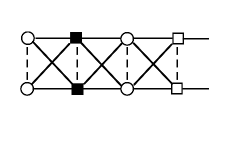
Figure 9: TBA diagram for the $sl(2/1)$ chain with alternating $3$ and $\bar{3}$ representations.

It is a simple matter to extend these results to a chain with alternating fully symmetric and antisymmetric representations, represented by Young diagrams with $p$ boxes . The TBA in universal form is represented by diagrams identical to the foregoing ones, only the massive nodes are the $2p^{th}$ ones. The central charge in the UV is $c={6p\over p+2}$.

It is also easy to extend the results to the case of the fundamental representation. The TBA now has source terms on the first nodes, as represented on figure 10. The UV central charge is $c=2$.

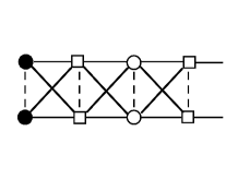
Figure 10: TBA diagram for the $OSP(2/2)$ chain (four dimensional fundamental representation).

The TBA for the spin chain confirms identifications of central charges carried out by other means in [8],[18]. Moreover, it constitutes a crucial check of completeness of the solutions of the Bethe ansatz equations, and we can now use our strings classification to tackle the more interesting problem of scattering in $osp(2/2)$ integrable quantum field theories.

Nevertheless, it is fair to remind the reader that the TBA is rather insensitive to details of the diagonalization. Consider for instance the well known $SU(2)$ spin 1/2 XXX chain. The total number of states with $S^{z}=0$ is $\Omega_{S^{z}=0}=\left(\begin{array}[]{c}L/2\\ L\end{array}\right)$ while the number of highest weight states with $j=0$ is $\Omega_{j=0}=\left(\begin{array}[]{c}L/2\\ L\end{array}\right)-=\left(\begin{array}[]{c}L/2-1\\ L\end{array}\right)$. However, if we consider the entropies associated with these two numbers we have

$$\ln\Omega_{j=0}=\ln\Omega_{S^{z}=0}-\ln{L+2\over 4}$$ (43)

so the difference is of order ${\ln L\over L}$ and goes to zero as $L\rightarrow\infty$. In other words, thermodynamics based on a scheme that would not provide all eigenstates but only the highest weight states say would still reproduce the expected results. In particular, even if our string analysis turns out to be wrong or incomplete for states in indecomposable representations, it is still very conceivable - as we indeed observe - that this effect is negligible in the thermodynamic limit.

A related comment concerns the reality condition we imposed on the densities of the two types of strings. Since evidence is strong that the minimum of the free energy functional is symmetric under the exchange of the two types of strings, our condition led us to what should be the correct result. It is not clear however how to describe solutions where there is a dissymmetry between type I and type II strange strings. Presumably, the string hypothesis breaks down in this case.

4 TBA for OSp(2$|$2) scattering: the fundamental representation case and the GN model

We now consider the different but related problem of writing up the TBA for the $OSp(2|2)$ GN model. The action is

$$S=\int{d^{2}x\over 2\pi}\left[\sum_{i=1}^{2}\psi^{i}_{L}\partial\psi^{i}_{L}+\psi^{i}_{R}\bar{\partial}\psi^{i}_{R}+\beta_{L}\partial\gamma_{L}+\beta_{R}\bar{\partial}\gamma_{R}+g\left(\psi^{1}_{L}\psi^{2}_{R}-\psi^{2}_{L}\psi^{1}_{R}+\gamma_{L}\beta_{R}-\beta_{L}\gamma_{R}\right)^{2}\right]$$ (44)

where the $\psi$ are Majorana fermions of conformal weight $1/2$, and the $\beta\gamma$ are bosonic ghosts of weight $1/2$ as well. The theory at $g=0$ can be identified with the $OSp(2|2)$ WZW model at level $k=1$ (part of the literature denotes this level $k=-1/2$ instead, focussing on the sub $SU(2)$). The lowest order beta function is $\beta(g)\propto-g^{2}$ and for $g<0$ the theory is massive . The corresponding S matrix has been proposed by Bassi and Leclair in [12]. It involves, as is usual for $O(N)$ GN models at large $N$ but not, a priori, at small $N$, particles of mass $M$ in the four dimensional fundamental representation, with scattering matrix of the form $S(\theta)=Z(\theta)R_{\hbox{fund}}(\theta)$ where $Z$ is a normalization factor, and $R_{\hbox{fund}}$ is the solution of the Yang Baxter equation for the fundamental representation, normalized such that the scattering kernel for particles in the highest weight state $b=0,S^{z}=1/2$ is equal to $Z$ (that is the matrix element in $R$ is equal to unity). The $R$ matrix is the same as the matrix defining the Boltzmann weights of the integrable spin chain. in the fundamental representation. The minimal $Z$ factor (in general we denote by $Z$ factor the element of the S matrix corresponding to diagonal scattering of two particles of the same type - no ambiguity will arise in what follows) given in [12] using standard crossing and unitarity arguments turns out to be the square of the similar factor for the $SU(2)_{1}$ WZW theory, or sine-Gordon model at $\beta^{2}=8\pi$,

$$Z=\left[{\Gamma\left(1+{i\theta\over 2\pi}\right)\Gamma\left({1\over 2}-{i\theta\over 2\pi}\right)\over\Gamma\left(1-{i\theta\over 2\pi}\right)\Gamma\left({1\over 2}+{i\theta\over 2\pi}\right)}\right]^{2}$$ (45)

Doubts were raised in [1] about this S matrix, on the grounds that, for $OSp(2|2)$ as for the usual $O(N)$ GN models at small $N$, the fundamental particles might well be kinks, while the fundamental fermions (and bosons in the super case) are unstable. It was suggested that maybe the S matrix of [12] in fact describes the sigma model $OSp(2|2)/OSp(1/2)$ instead. We will, in what follows, find evidence that this expectation is not correct, and that the S matrix of [12] does indeed describe the GN model. Of course, writing the TBA for the scattering theory is not the same as writing it for the integrable spin chain, as the number of particles is allowed to fluctuate. The two problems are however closely related, as is well known (see [19] for a pedagogical discussion)

The problem of quantizing the particles turns, in the continuous limit, into the basic equation

$$2\pi(\sigma+\sigma^{h})=M\cosh\theta+{1\over i}{d\over d\theta}\ln Z\star\sigma+{1\over i}{d\over d\theta}\ln\Lambda$$ (46)

Here $\Lambda$ is the eigenvalue of the monodromy matrix, ie of the matrix describing the process of passing one particle through a system with a certain number of particles already. This eigenvalue (properly normalized, so that it is equal to unity if all particles are of the same type, corresponding to ‘all spins up’ in the auxiliary problem) is found itself by another, ‘auxiliary’ Bethe ansatz, which coincides with the one used to diagonalize the spin chain. We need the general formula for the eigenvalue picked up when passing a particle of rapidity $v$ through a set of particles with rapidities $\{v_{A}\}$

$$\Lambda(v|\{v_{A}\})=\prod{v-u_{j}+i/2\over v-u_{j}-i/2}{v-\gamma_{\alpha}+i/2\over v-\gamma_{\alpha}-i/2}$$ (47)

(one checks that its logarithmic derivative gives the energy for the hamiltonian in the previous section), where the $u,\gamma$ are related to the $\{v_{A}\}$ through the Bethe equations

$$\prod_{A}{u_{j}-v_{A}+i/2\over u_{j}-v_{A}-i/2}=\prod_{\beta=1}^{M}{u_{j}-\gamma_{\beta}+i\over u_{j}-\gamma_{\beta}-i},~{}~{}~{}j=1,\ldots,N$$

$$\prod{\gamma_{\alpha}-v_{A}+i/2\over\gamma_{\alpha}-v_{A}-i/2}=\prod_{k=1}^{N}{\gamma_{\alpha}-u_{k}+i\over\gamma_{\alpha}-u_{k}-i},~{}~{}~{}\alpha=1,\ldots,M$$ (48)

Note that the same set of rapidities $\{v_{A}\}$ is used in both equations for the $u$ as well as the $\gamma$’s. Here we have used the lattice rapidities for the auxiliary problem to match with the previous section. They are related to the relativistic ones by $\theta=\pi u$. We define the Fourier transformation for functions of $\theta$ as

$$\hat{f}(x)=\int d\theta e^{i\theta x/\pi}f(\theta)$$ (49)

The Bethe equations for the auxiliary system (48) admit the same clasification of roots as the one for the lattice model, and lead therefore to the following system

$$\rho_{I,n}^{w}+\hat{\rho}_{I,n}^{w} = a_{2n-1}\star\sigma+\sum_{p}\Phi_{I,n;I,p}^{w;w}\star\rho_{I,p}^{w}+\Phi_{I,n;II,p}^{w;w}\star\rho_{II,p}^{w}$$

$$+ \Phi_{I,n;I,p}^{w;s}\star\rho_{I,p}^{s}+\Phi_{I,n;I,p}^{w;s}\star\rho_{II,p}^{s}$$

$$\rho_{I,n}^{s}+\hat{\rho}_{I,n}^{s} = a_{2n}\star\sigma+\sum_{p}\Phi_{I,n;I,p}^{s;w}\star\rho_{I,p}^{w}+\Phi_{I,n;II,p}^{s;w}\star\rho_{II,p}^{w}$$ (50)

$$+ \Phi_{I,n;I,p}^{s;s}\star\rho_{I,p}^{s}+\Phi_{I,n;I,p}^{s;s}\star\rho_{II,p}^{s}$$

and a similar equation for type II roots (the kernels $\Phi$ have been defined in the previous sections). As for the $\sigma$ equations they are

$$\sigma+\sigma^{h}={M\over 2\pi}\cosh\theta+{1\over 2i\pi}{d\over d\theta}\ln Z\star\sigma-\sum_{k\geq 1}a_{2k-1}\star(\rho_{I,k}^{w}+\rho_{II,k}^{w})$$

$$-\sum_{k\geq 1}a_{2k}\star(\rho_{I,k}^{s}+\rho_{II,k}^{s})$$ (51)

where we now define

$$a_{t}(\theta)={i\over 2\pi}{d\over d\theta}\ln{\theta+i\pi t/2\over\theta-i\pi t/2}$$ (52)

and all the densities are now in terms of the (physical or auxiliary) rapidities.

We write symbolically our system as

$$\rho_{I,i}+\rho_{I,i}^{h}=\Phi_{I,i;\sigma}\star\sigma+\sum_{j}\Phi_{I,i;I,j}\star\rho_{I,j}+\Phi_{I,i;II,j}\star\rho_{II,j}$$

$$\rho_{II,i}+\rho_{II,i}^{h}=\Phi_{II,i;\sigma}\star\sigma+\sum_{j}\Phi_{II,i;I,j}\star\rho_{I,j}+\Phi_{II,i;II,j}\star\rho_{II,j}$$

$$\sigma+\sigma^{h}={M\cosh\theta\over 2\pi}+\Phi_{\sigma,\sigma}\star\sigma+\sum_{i}\Phi_{\sigma;I,i}\star\rho_{I,i}+\Phi_{\sigma;II,i}\star\rho_{II,i}$$ (53)

and the labels $i,j$ are short hands for $n,p$ and $s,w$. We analyze then the thermodynamics of this system, with the energy

$${E\over L}=\int\sigma(\theta)M\cosh\theta d\theta$$ (54)

Introducing pseudoenergies through $\rho^{h}/\rho=e^{\epsilon_{n}/T}$, $\sigma^{h}/\sigma=e^{\epsilon_{\sigma}/T}$, we find the TBA equations

$$\epsilon = M\cosh\theta-T\Phi_{\sigma,\sigma}\star\ln\left(1+e^{-\epsilon_{\sigma}/T}\right)-T\sum_{i}\Phi_{I,i;\sigma}\star\ln\left(1+e^{-\epsilon_{I,i}/T}\right)$$

$$- T\Phi_{II,i;\sigma}\star\ln\left(1+e^{-\epsilon_{II,i}/T}\right)$$

$$\epsilon_{I,i} = -T\Phi_{\sigma;I,i}\star\ln\left(1+e^{-\epsilon_{\sigma}/T}\right)-T\sum_{j}\Phi_{I,j;I,i}\star\ln\left(1+e^{-\epsilon_{I,j}/T}\right)$$

$$- T\sum_{j}\Phi_{II,j;I,i}\star\ln\left(1+e^{-\epsilon_{II,j}/T}\right)$$

$$\epsilon_{II,i} = -T\Phi_{\sigma;II,i}\star\ln\left(1+e^{-\epsilon_{\sigma}/T}\right)-T\sum_{j}\Phi_{I,j;II,i}\star\ln\left(1+e^{-\epsilon_{I,j}/T}\right)$$ (55)

$$- T\sum_{j}\Phi_{II,j;II,i}\star\ln\left(1+e^{-\epsilon_{II,j}/T}\right)$$

while

$${F\over L}=-T\int{M\cosh\theta\over 2\pi}\ln\left(1+e^{-\epsilon_{\sigma}/T}\right)d\theta$$ (56)

Observing now that $\Phi_{\sigma;I,i}=\Phi_{\sigma;II,i}\equiv\Phi_{\sigma,i}$, we expect that $\epsilon_{I,i}=\epsilon_{II,i}\equiv\epsilon_{i}$ at equilibrium, and thus get a new system

$$\epsilon_{i}=-\sum_{j}T(\Phi_{I,j;I,i}+\Phi_{II,j;I,i})\star\ln\left(1+e^{-\epsilon_{j}/T}\right)-T\Phi_{\sigma;i}\star\ln\left(1+e^{-\epsilon_{\sigma}/T}\right)$$

$$\epsilon_{\sigma}=M\cosh\theta-T\Phi_{\sigma,\sigma}\star\ln\left(1+e^{-\epsilon_{\sigma}/T}\right)-2T\sum_{i}\Phi_{i;\sigma}\star\ln\left(1+e^{-\epsilon_{i}/T}\right)$$ (57)

Remarkably, this TBA is identical with the TBA one would write for the $SU(2)$ PCM model [20]. There, the scattering matrix is the product of two $SU(2)$ isotropic sine-Gordon scattering matrices, and the strings involved in diagonalizing each of the two scattering matrices behave like our type $I$ and type $II$ solutions.

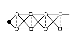
Figure 11: TBA diagram for the $OSP(2/2)$ theory with particles in the fundamental representation.

Identifying the nodes of type I and type II and using the fact that the pseudoenergies are equal in equilibrium gives the equivalent diagrams shown in 12.

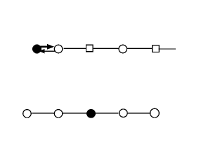
Figure 12: Equivalent TBA diagrams for the $OSP(2/2)$ theory with particles in the fundamental representation, showing mapping to the $SU(2)$ PCM model.

We conclude that $c_{UV}=3$, for our scattering theory. This is in agreement with the effective central charge for the GN model in the sector with anti-periodic fermions (NS), and provides some justification for the S matrix of [12].

If we now accept that the S matrix in [12] is the correct one, it follows from our calculation that the free energy of the $OSP(2/2)$ GN model in the NS sector is exactly equal to the one of the $SU(2)$ PCM model. Now note the latter is the same as the $SO(4)/SO(3)$ sigma model: we thus have established part of the equivalences expected from the introduction.

Our observation deserves several remarks. The first is, that the torus partition function of the free GN model with periodic boundary conditions for the fermions is exactly equal to unity. This results from the cancellation between the fermionic and bosonic contributions (each equal to $\hbox{Det }\Delta^{\pm 1}$, $\Delta$ the Laplacian), and is in fact what motivates the appearance of the $OSp(2|2)$ symmetry in the SUSY approach to disordered systems. One can easily show that this supersymmetry is not broken by the introduction of a current-current perturbation. The partition function with periodic BC should thus remain unity, which implies in particular that the bulk term in the free energy - which does not depend on the boundary conditions - should vanish exactly. Turning now to the non trivial sector with antiperiodic boundary conditions for the fermions, the free energy now becomes the non trivial object we have studied in this section, but its bulk part should still vanish exactly. Since we have argued the free energy for the $OSp(2|2)$ GN model should coincide with the one of the $SU(2)$ PCM, this implies the bulk term must vanish there. To calculate this bulk term, we use the fact that $SU(2)$ PCM coincides with the $O(4)$ sigma model. The bulk term for $O(N)$ sigma models follows from the general results in [21],[22],[23]:

$${F^{(0)}\over L}={M^{2}\over 8}\cot{\pi\over N-2}$$ (58)

where $M$ is the lowest mass. We conclude that for the $SU(2)$ PCM, for which $N=4$:

$${F^{(0)}\over L}={M^{2}\over 8}\times 0$$ (59)

in agreement with our expectation for $OSp(2|2)$.

5 The OSp(2$|$2) supersphere sigma model TBA.

If the S matrix proposed in [12] is for the GN model indeed, the question is now open as to what the S matirx of the sigma model might be. By analogy with what happens for $O(N)$, $N>0$, and after switching the roles of GN and $\sigma$M, one would expect that the S matrix for the $OSp(2|2)$ sigma model should involve spinor representations. This could be the three dimensional representations (fundamental of $SL(2|1)$ and its conjugate), or maybe some infinite dimensional representations[24]. Our naive attempts in this direction have not been successful however.

An alternative approach consists in starting from lattice regularizations. It was indeed argued in [1] that the continuum limit of the integrable staggered $OSp(2|2)$ chain built on the fundamental was described by the $OSp(2|2)/OSp(1|2)$ sigma model in the massive regime. The staggering is similar to what has been studied in particular under the name of lattice light cone regularization for a large class of perturbed CFTs and sigma models [25][26]. For a recent reference in a very similar case, see [27].

Recall that, for the integrable chain based on the four dimensional representation, the bare source term involves a factor ${i\over 2}$ instead of $i$, and as a result, the source term for the wide and strange strings are different:

$$\hat{s}^{w}_{I,n} = \hat{s}^{w}_{II,n}=a_{2n-1}$$

$$\hat{s}^{s}_{I,n} = \hat{s}^{s}_{II,n}=a_{2n}$$ (60)

(so in general we can write that the source term of a string with $p$ roots is $a_{p}$).

What we have to do, following the general ideas of [1],[27] is to consider instead of the homogeneous chain, the chain arising from staggering spectral parameters. The relevant equations now read

$$\left({u_{j}+\Lambda/2+i/2\over u_{j}+\Lambda/2-i/2}\right)^{L/2}\left({u_{j}-\Lambda/2+i/2\over u_{j}-\Lambda/2-i/2}\right)^{L/2}=\prod_{\beta=1}^{M}{u_{j}-\gamma_{\beta}+i\over u_{j}-\gamma_{\beta}-i},~{}~{}~{}j=1,\ldots,N$$

$$\left({\gamma_{\alpha}+\Lambda/2+i/2\over\gamma_{\alpha}+\Lambda/2-i/2}\right)^{L/2}\left({\gamma_{\alpha}-\Lambda/2+i/2\over\gamma_{\alpha}-\Lambda/2-i/2}\right)^{L/2}=\prod_{k=1}^{N}{\gamma_{\alpha}-u_{k}+i\over\gamma_{\alpha}-u_{k}-i},~{}~{}~{}\alpha=1,\ldots,M$$ (61)

with the quantum numbers $B={N-M\over 2}$and $J^{3}=L-{M+N\over 2}$. The energy reads then

$$E\propto-\left(\sum_{k=1}^{N}{1\over(u_{k}-\Lambda/2)^{2}+1/4}+{1\over(u_{k}+\Lambda/2)^{2}+1/4}+\sum_{\beta=1}^{M}{1\over(\gamma_{\beta}-\Lambda/2)^{2}+1/4}+{1\over(\gamma_{\beta}+\Lambda/2)^{2}+1/4}\right)$$ (62)

The ground state of the system was discussed in [8, 18] and was shown to consist of filled up sea of real roots (ie $n=1$ wide strings) of type I and type II. Excitations can easily be shown (see more details below) to be massive, with a mass scale $Ma\propto e^{-\pi\Lambda/2}$, with $a$ the lattice spacing, so the continuum limit is obtained as usual with $a\rightarrow 0$, $\Lambda\rightarrow\infty$. From the general discussion in the second section, it follows that the ground state energy is given by twice the ground state energy of the staggered XXX chain. But for the latter, the ground state energy is well known to reproduce, in the continuum limit where $\Lambda\rightarrow\infty$, the ground state energy of the $SU(2)_{1}$ WZW model perturbed by the current current interaction, or, equivalently, of the sine-Gordon model at $\beta_{SG}^{2}=8\pi$.

It is also a well known fact that the $SO(4)$ GN model is equivalent to two decoupled sine Gordon models at their marginal point [28]. We thus have obtained our other claim, namely that the free energy of the $OSp(2|2)$ supersphere sigma model with antiperiodic boundary conditions coincides with the free energy of the $SO(4)$ GN model.

We thus have coincidence of free energies as

$$OSP(2/2)\hbox{ GN }\leftrightarrow SO(4)/SO(3)\hbox{ sigma Model }\equiv SU(2)\times SU(2)\hbox{ PCM}$$

$$OSP(2/2)/OSP(1/2)\hbox{ supersphere sigma Model }\leftrightarrow SO(4)\hbox{ GN}\equiv SU(2)\times SU(2)\hbox{ GN}$$ (63)

We note however that the relationship does not seem to extend to the full spectra of the theories. We haven’t been able to find an $SU(2)\times SU(2)$ symmetry within either of the $OSP(2/2)$ models for instance. The UV limits of the flows are quite different as well. For instance the UV limit of the $SO(4)$ GN is compact, while the UV limit of the $OSP(2/2)$ supersphere sigma model has a non compact direction.

Now we can get back to the question of what the S matrix might be. For ordinary models, this can be rather easily determined using the Bethe equations from the lattice regularization. The idea is to rewrite the continuous Bethe ansatz equations in terms of excitations over the vacuum [29], ie by putting on the right hand side, not densities of $n=1$ wide strings, but densities of $n=1$ holes in the wide strings ground state distribution, that is replace $\rho_{I,1}$ and $\rho_{II,1}$ by $\rho_{I,1}^{w,h}$ and $\rho_{II,1}^{w,h}$.

After laborious but straightforward calculations, one ends up with the following equations for the densities of real particles (we denote $\sigma_{I}\equiv\rho_{I,1}^{w}$ and similarly for type II)

$$\widehat{\sigma}_{I}+\widehat{\sigma}_{I}^{h} = {\cosh\Lambda x/2\over 2\cosh(x/2)}-{e^{-|x|}\over 2\sinh|x|}\widehat{\sigma}_{I}^{h}+{1\over 2\sinh|x|}\widehat{\sigma}_{II}^{h}-\sum_{k\geq 2}e^{-(k-1)|x|}\widehat{\rho}_{I,k}^{w}$$

$$- \sum_{k\geq 1}e^{-(k-1/2)|x|}\left({1+\hbox{sign }(x)\over 2}\widehat{\rho}_{I,k}^{s}+{1-\hbox{sign }(x)\over 2}\widehat{\rho}_{II,k}^{s}\right)$$

$$\widehat{\sigma}_{II}+\widehat{\sigma}_{II}^{h} = {\cosh\Lambda x/2\over 2\cosh(x/2)}-{e^{-|x|}\over 2\sinh|x|}\widehat{\sigma}_{II}^{h}+{1\over 2\sinh|x|}\widehat{\sigma}_{I}^{h}-\sum_{k\geq 2}e^{-(k-1)|x|}\widehat{\rho}_{II,k}^{w}$$ (64)

$$- \sum_{k\geq 1}e^{-(k-1/2)|x|}\left({1+\hbox{sign }(x)\over 2}\widehat{\rho}_{II,k}^{s}+{1-\hbox{sign }(x)\over 2}\widehat{\rho}_{I,k}^{s}\right)$$

For the other solutions, one observes that the bare source terms disappear, and are replaced by source terms which are convolutions involving the densities $\sigma_{I}^{h}$ and $\sigma_{II}^{h}$. As for the interactions between different types of roots, one finds that a shift of one unit in the length is taking place. That is, what was before an $n$ ($n>1$) wide root of type I or II now behaves as an $n-1$ strange root of type I or II, while what was before a strange $n$ root of type I or II now behaves as an $n$ wide root of type I or II. In other words, we have the following system

$$\widehat{\rho}_{I,k}^{w}+\widehat{\rho}_{I,k}^{w,h} = e^{-(k-1)|x|}\widehat{\sigma}_{I}^{h}+\sum_{l\geq 2}D\widehat{\Phi}^{w,w}_{I,k;I,l}\star\widehat{\rho}_{I,l}^{w}+\ldots$$

$$\widehat{\rho}_{II,k}^{w}+\widehat{\rho}_{II,k}^{w,h} = e^{-(k-1)|x|}\widehat{\sigma}_{II}^{h}+\sum_{l\geq 2}D\widehat{\Phi}^{w,w}_{II,k;I,l}\star\widehat{\rho}_{I,l}^{w}+\ldots$$

$$\widehat{\rho}_{I,k}^{s}+\widehat{\rho}_{I,k}^{s,h} = e^{-(k-1/2)|x|}\left({1+\hbox{sign}(x)\over 2}\widehat{\sigma}_{I}^{h}+{1-\hbox{sign}(x)\over 2}\widehat{\sigma}_{II}^{h}\right)++\sum_{l\geq 2}D\widehat{\Phi}^{s,w}_{I,k;I,l}\star\widehat{\rho}_{I,l}^{w}+\ldots$$

$$\widehat{\rho}_{II,k}^{s}+\widehat{\rho}_{II,k}^{s,h} = e^{-(k-1/2)|x|}\left({1+\hbox{sign}(x)\over 2}\widehat{\sigma}_{II}^{h}+{1-\hbox{sign}(x)\over 2}\widehat{\sigma}_{I}^{h}\right)++\sum_{l\geq 2}D\widehat{\Phi}^{s,w}_{II,k;I,l}\star\widehat{\rho}_{I,l}^{w}$$ (65)

where each time the dots indicate the obvious sum over the remaining terms $(I,s),(II,w),(II,s)$, and the dressed kernels are obtained by shifts

$$D\Phi_{I,n;I,p}^{w,w}=\Phi_{I,n-1;I,p-1}^{s,s}\ldots$$ (66)

The new system bears a lot of resemblance with the old one. In fact, up to a relabelling of the roots, it is identical for what concerns the interactions between the densities $\rho$ of pseudoparticles.

This is fully expected, since the dynamics of the $\rho$ excitations is determined entirely by the symmetries of the model - here, $osp(2|2)$ super Lie algebra.

Now for the interaction between the sigma densities. In the case of ordinary Lie algebras - say $sl(3)$, of rank two like our present TBA - the holes in $\sigma_{I,II}$ distributions would be associated with particles living in the representations corresponding to the first top or bottom node of the TBA diagram. Oddly enough, while this would be fine if we were considering the second nodes on the diagram (which correspond, as we have seen earlier, to $3,\bar{3}$), there is no $osp(2|2)$ representation corresponding to the first nodes individually! A quick calculation shows that these representations should have dimension $\sqrt{4}=2$ indeed, and this is not possible in $osp(2|2)$. This might indicate that the full $osp(2|2)$ symmetry is not present in the S matrix, but maybe only a sub $sl(2)\times sl(2)$.

However, it should also be clear that the kernels for $I-I$ and $I-II$ interactions are also quite ill behaved, as their Fourier transforms both diverge at the origin:

$${1\over i}{d\over d\theta}\ln Z_{I,I}={1\over i}{d\over d\theta}\ln Z_{II,II}=-{1\over\pi}\int dx{e^{-|x|}\over 2\sinh|x|}e^{-i\theta x/\pi}$$

$${1\over i}{d\over d\theta}\ln Z_{I,II}={1\over i}{d\over d\theta}\ln Z_{II,I}={1\over\pi}\int dx{1\over 2\sinh|x|}e^{-i\theta x/\pi}$$ (67)

(here, $\theta$ is the usual physical rapidity, obtained from the lattice rapidity through a rescaling). We believe this divergence is related with the non-compactedness of the target space in the UV limit; this will be discussed in more details in the next section.

Meanwhile, it is intriguing to observe that, if we were to define new excitations by binding a hole in the distribution of real wide roots of type I and a hole in the distribution of wide roots of type II at the same rapidity, the Fourier transform of the derivative of the logarithm of the dressed scattering kernel of these new excitations with themshelves would be

$$\widehat{\Phi}_{I+II,I+II}=2\left({1\over 2\sinh|x|}-{e^{-|x|}\over 2\sinh|x|}\right)={e^{-|x|/2}\over\cosh|x|/2}$$ (68)

Similarly the kernel of such an excitation with a wide string of type I or type II is given by $e^{-(k-1)|x|}$ while the kernel of such an excitation with a strange string of type I or II is given by $e^{(k-1/2)|x|}$. Hence, if we forced holes in the I and II distributions to be bound, the following system of equations deduced from the lattice model would now coincide with the TBA of the previous section provided we identify

$$2\pi\Phi_{\sigma,\sigma}={1\over i}{d\over d\theta}\ln Z={1\over\pi}\int_{-\infty}^{\infty}{e^{-|x|/2}\over\cosh(x/2)}e^{-i\theta x/\pi}dx$$ (69)

Integrating this quantity we find

$$Z=(Z_{I,I}Z_{I,II})^{2}=\left[{\Gamma\left(1+{i\theta\over 2\pi}\right)\Gamma\left({1\over 2}-{i\theta\over 2\pi}\right)\over\Gamma\left(1-{i\theta\over 2\pi}\right)\Gamma\left({1\over 2}+{i\theta\over 2\pi}\right)}\right]^{2}$$ (70)

which in fact is the result for the GN model discussed above. In other words, pairs of holes in the I and II distributions at identical rapidities in the sigma model scatter exactly with the GN S matrix! There is however no obvious reason why these holes should be paired (and the sigma model does not coincide with the GN model anyhow), so the sigma model S matrix appears as some sort of ‘split’ GN S matrix. More work on the bound states and crossing unitarity would be necessary to give sense to this idea.

We note here that in the case $N>0$, the generic sigma model S matrix gives the correct scattering theory for all values of $N$, while the generic GN S matrix works only for large enough $N$; at small enough $N$, the fundamental fermions are unstable, and the correct S matrix involves instead kinks in the spinor representations. It seems that for $N\leq 0$, the roles of the GN and sigma model are switched again: the generic S matrix for GN seems to still work for $N=0$, while for the sigma model at $N=0$, some sort of ‘spinor’ S matrix seems necessary. The spinor representations of $OSp(2|2)$ are however infinite dimensional, and it is not clear whether they would allow for a meaningful description of the scattering in the present case.

We note finally that the ground state energy of the $OSp(2|2)$ sigma model can be calculated using the general result (58) with $N=0$ and one finds again

$${F\over L}=-{M^{2}\over 8}\times 0$$ (71)

This agrees with the ground state energy for the WZW model perturbed by current current interaction [30].

6 Do the massive flows exist?

A important remark is that, according to the discussion in [31], the $OSp(2|2)$ WZW model perturbed by a current current interaction in the massive direction in fact does not exist as a field theory. More precisely, it is established in this reference that the functional integral is not well defined, the topological term leading to strong divergences.

The same holds true, in fact, for the sigma model, as was briefly discussed in [32]. The action for the supersphere $OSP(2/2)/OSP(1/2)$ sigma model is obtained as follows. Parameterize the $S^{1,2}$ supersphere as

$$\phi_{1} = \cos\phi\left(1-\eta_{1}\eta_{2}\right)$$

$$\phi_{2} = \sin\phi\left(1-\eta_{1}\eta_{2}\right)$$ (72)

such that $\phi_{1}^{2}+\phi_{2}^{2}+2\eta_{1}\eta_{2}=1$. The action is then

$$S={1\over g}\int{\rm d}^{2}x\,\left[\left(\partial_{\mu}\phi\right)^{2}(1-2\eta_{1}\eta_{2})+2\partial_{\mu}\eta_{1}\partial_{\mu}\eta_{2}-4\eta_{1}\eta_{2}\partial_{\mu}\eta_{1}\partial_{\mu}\eta_{2}\right]$$ (73)

where $\phi$ is compactified, $\phi\equiv\phi+2\pi$, and conventions such that the Boltzmann weight is $e^{-S}$. The spontaneously broken symmetry phase, with the theory being free in the UV and massless in the IR, corresponds to a positive coupling constant $g$, since for the $O(N)$ model, the beta function is

$${dg\over dl}=\beta(g)=(N-2)g^{2}$$ (74)

and the same holds for $OSp(n|2m)$ sigma models with $N\equiv n-2m$. When $g$ is positive, the theory flows to weak coupling, and critical properties are described by the $g\rightarrow 0$ limit. A rescaling and relabeling brings the action into the form

$$S=\int{\rm d}^{2}x\,\left[\left(\partial_{\mu}\phi\right)^{2}(1-2g\eta_{1}\eta_{2})+2\partial_{\mu}\eta_{1}\partial_{\mu}\eta_{2}-4g\eta_{1}\eta_{2}\partial_{\mu}\eta_{1}\partial_{\mu}\eta_{2}\right]$$ (75)

with now $\phi\equiv\phi+{2\pi\over\sqrt{g}}$. As $g\rightarrow 0$, we thus obtain a symplectic fermion and a non-compact boson.

Note that the presence of a continuous spectrum in this $osp(2/2)$ version of the problem has a physical origin in the fact that the symmetry is spontaneously broken, and thus correlation functions of order parameters have no algebraic decay (though they have non trivial logarithmic behaviour).

Now the massive region meanwhile corresponds to the theory flowing to strong coupling, and $g$ negative. Except in the $OSp(1|2)$ case, where there is a single bosonic field, and the theory can be reformulated entirely in terms of the symplectic fermions, in the $OSp(2|2)$ case in particular, a negative coupling constant leads to a term $\exp\left[+\int d^{2}x(\partial_{\mu}\phi)^{2}\right]$ in the Boltzmann weight, and thus to a theory that is not well defined from the path integral point of view. We note that trying to define theories in a region where the path integral is not defined is a task that has been considered in string theory for some time. An example is the so called “time like Liouville theory”, discussed for instance in [33] and [34].

So what happens at $g$ negative and the “massive” region is not entirely clear. The model defined by the action (73) is unstable, a fact that probably manifests itself by a spectrum that becomes unbounded from below, and hence level crossing right at $g=0$.

The point can be illustrated more concretely in the case of the $OSp(4|2)$ GN model. In the papers [5] and [6] it was found that, for the sign of the $O(N)$ GN coupling which corresponds to the relevant direction in the case $N>2$, the model is gapless and exhibits a line of fixed points with central charge $c=1$. Meanwhile, for the opposite sign of the coupling, something very different occurs. This can best be seen by contemplating the formula giving the exact values of the conformal weights and thus the scaled gaps on the critical line (for the theory with Neumann boundary conditions), as a function of the Young diagrams for the $OSp(4|2)$ representations. Writing the weights at the free point as

$$h_{\hbox{free}} = {n_{1}^{2}\over 2}+{n_{2}^{2}\over 2}+{b-2\over 2},~{}~{}b\geq 2$$

$$h_{\hbox{free}} = {n_{1}^{2}\over 2},~{}~{}b=0,1$$ (76)

for a Young diagram with shape $\lambda=n_{1}n_{2}1^{b-2}$, the exact formula [5, 6] is

$$h=h_{\hbox{free}}+gC$$ (77)

where $C$ is the Casimir of the representation

$$C={(n_{1}+n_{2}-1)^{2}\over 2}+{(n_{1}-n_{2}+1)^{2}\over 2}-(b-1)^{2}$$ (78)

While for $g>0$ the ground state remains in the identity sector, for $g<0$, the weights of the fully antisymmetric representations $1^{p}$ (for instance) become arbitrarily large and negative for $p=O(1/\sqrt{g})$ as soon as $g$ is turned on: an infinity of crossings occurs, and the new ground state has nothing to do with the one at $g<0$.

On the other hand, we could also restrict to the $O(2)$ subsector of the theory. There, the partition function is the one of the free boson with Neumann boundary conditions, and nothing happens - since all the representations which could cross the ground state are eliminated when going from $OSp(4|2)$ to the sub $O(2)$. The properties of the ground state, analytically continued in this phase, are well behaved, but describe a subset of the theory which is very high in energy. The equivalent observation in the $OSp(2|2)$ GN model would correspond to the sector with periodic boundary conditions, where the partition function remains equal to unity and $c=0$; this sector might be very high in energy with respect to the true ground state in the would be massive phase.

The $OSp(2|2)$ sigma model can be studied somewhat in the same spirit by using perturbation theory. Near the weak coupling fixed point, the massive direction formally corresponds to negative $g$, and, if we for a minute do not worry about the meaning of the path integral, we can calculate the evolution of the hamiltonian eigenvalues perturbatively. Symmetric representations are particularly easy to handle, since they can also be obtained through the minisuperspace analysis. The eigenvalues are simply proportional to those of the Laplacian on the supersphere:

$$H=g\Delta_{S^{-1}}$$ (79)

and of the form $E=gn(n-2)$, $n$ an integer. They all collapse at $g=0$, and there is an infinity of level crossings at that point when going from $g$ positive to $g$ negative.

We note that, if this scenario is correct, the point $g=0$ must be considered as a ‘first order critical point”. This is a point where the theory is conformal invariant, but which is at the same time a point where level crossing occurs, such that the analytic continuation of the ground state becomes a very highly excited state in the low temperature phase. In general, first order phase transitions are not associated with conformal field theories, but several examples of first order critical points are known. These involve crossings in finite size, and are only possible because of the non unitarity. Maybe the best studied example corresponds to the thermal perturbation of the antiferromagnetic Potts model on the square lattice, as discussed in [18].

Meanwhile, we have a lattice regularization (the staggered spin chain) and a TBA that seem perfectly stable. In particular, we have not found, by exploring solutions which are dissymmetric in the two types of roots I and II, any indication that the ground state of the chain is not given by the foregoing results. It looks thus as if our results describe some sort of continuation of the unstable theory, which now behaves as an (almost) ordinary massive theory. It would of course be interesting to explore this issue in more details.

7 The q-deformed case

We have so far discussed only the case of twisted boundary conditions for the fermions, corresponding to the “effective” central charge of our non unitary theories. To get the true central charge, one must consider a twisted TBA, by inserting (complex) chemical potentials for the kinks in the scattering. For the $OSp(2|2)$ GN model, we do not expect that much interesting will remain. The central charge will be zero in the UV, it is zero in the IR for the massive flow, and probably remains zero all the way.

The situation is more interesting for the supersphere sigma model, since now $c=-1$ in the UV. To get the calculation of the true central charge under control, it is convenient to consider the q deformed version of our problem.

In terms of lattice model, the q-deformation is obtained by taking the four dimensional solution of the YB equation based on $U_{q}OSp(2|2)$ [35].

Setting $q=e^{i\xi}$ we have the Bethe equations for a chain with $L$ sites

$$\left({\sinh{1\over 2}(U_{j}-i\xi)\over\sinh{1\over 2}(U_{j}+i\xi)}\right)^{L}=\prod_{\beta}{\sinh{1\over 2}(U_{j}-\Gamma_{\beta}-2i\xi)\over\sinh{1\over 2}(U_{j}-\Gamma_{\beta}+2i\xi)}$$

$$\left({\sinh{1\over 2}(\Gamma_{\beta}-i\xi)\over\sinh{1\over 2}(\Gamma_{\beta}+i\xi)}\right)^{L}=\prod{\sinh{1\over 2}(\Gamma_{\beta}-U_{j}-2i\xi)\over\sinh{1\over 2}(\Gamma_{\beta}-U_{j}+2i\xi)}$$ (80)

(the isotropic limit is recovered by setting $U_{j}=2\xi u_{j},\Gamma_{\beta}=2\xi\gamma_{\beta}$ and $\xi\to 0$. The energy of the chain is meanwhile

$$E\propto-\left(\sum_{k}{\sin\xi\over\cosh U_{j}-\cos\xi}+\sum_{\beta}{\sin\xi\over\cosh\Gamma_{\beta}-\cos\xi}\right)$$ (81)

In the antiferromagnetic regime $\xi\in[0,{\pi\over 2}]$, the ground state is obtained by filling up the seas $y_{I},y_{II}$ with real roots. With anti-periodic boundary conditions for the fermionic degrees of freedom (the NS sector), the central charge reads $c_{\hbox{eff}}=2$.

The most natural is to observe that the XXZ sub component of the spectrum (that is, the component given by $y_{I}=y_{II}$) can be twisted to obtain a $c<1$ theory described by a Coulomb gas with parameter $\alpha_{0}$. To do so we impose boundary conditions twisted by $e^{2i\pi\phi}$ on the spins, $\phi={\xi\over\pi}$ resulting in the central charge for the XXZ chain

$$c=1-{6(\xi/\pi)^{2}\over 1-(\xi/\pi)}$$ (82)

We now parametrize

$${\xi\over\pi}={1\over 2l+3}$$ (83)

(usually one would set $\xi/\pi=1/(m+1)$) so the central charge of the $OSp$ chain becomes

$$c_{\hbox{twist1}}=2\left[1-{6\over(2l+2)(2l+3)}\right]$$ (84)

Meanwhile, we recall that the effective central charges (ie, describing the ground state scaling in the NS sector) of the $OSp(2|2)$ and $OSp(1|2)$ WZW theories at level $l$ read

$$OSp(2|2)_{l};~{}~{}c=0;~{}~{}c_{\hbox{eff}}={6l\over l+1}$$

$$OSp(1|2)_{l};~{}~{}c={2l\over 2l+3};~{}~{}c_{\hbox{eff}}={8l\over 2l+3}$$ (85)

It is easy to check that

$$c_{\hbox{twist1}}={6l\over l+1}-{8l\over 2l+3}$$ (86)

This suggests that the continuum limit of the spin chain is described, for $l$ integer, by coset models $OSp(2|2)_{l}/OSp(1|2)_{l}$ and suitable interpolations in between.

When one goes from the XXZ to the minimal models, a set of electric charges have to be introduced, which are multiple of the fundamental charge $e_{0}={\gamma\over\pi}$. The particular choice $e=(l+1)e_{0}$ gives the conformal weight, with respect to the central charge of the minimal model,

$$h_{t}={(l+1)^{2}-1\over 4(2l+2)(2l+3)}$$

This leads to an effective central charge for the $OSp$ theory

$$c_{\hbox{twist2}}=c_{\hbox{twist1}}-24\times 2\times h=-{2l\over 2l+3}$$ (87)

which is the true central charge of the coset model. The phase shift to obtain this central charge is thus $\exp[2i\pi(l+1)/(2l+3)]$; it becomes a pure $e^{i\pi}$ in the $l\rightarrow\infty$ limit, where the central charge $c_{\hbox{twist2}}$ becomes equal to $-1$.

A way to obtain the flow of the central charge in the supersphere sigma model is thus to take the flow of the running dimension in the minimal models $M_{2l+2,2l+3}$ in the limit $l\rightarrow\infty$.

Now this is particularly simple. Indeed, we observe that $h_{t}=h_{l+1,l+1}$, and the running dimension of operators $\Phi_{rr}$ in minimal models is the easiest to obtain, since it follows from a simple twist on the basic sine-Gordon equations. This can be done in the context of the TBA, as discussed in [36]. In the notations of this paper, one must set $\gamma={1\over 2}$, so the soliton fugacities are $\exp[\pm i\pi(2l+3)/2]$. One can also use the DDV formalism, and for instance the formulas in [37]. The basic equations reads

$$f(\theta)=imR\sinh\theta+i\alpha+\int_{C_{1}}\Phi(\theta-\theta^{\prime})\ln\left(1+e^{f(\theta^{\prime})}\right)d\theta^{\prime}+\int_{C_{2}}\Phi(\theta-\theta^{\prime})\ln\left(1+e^{-f(\theta^{\prime})}\right)d\theta^{\prime}$$ (88)

where $\Phi$ is the SG kernel for the corresponding value of the sine-Gordon coupling, ${\beta_{\rm SG}^{2}\over 8\pi}=1-{1\over 2l+3}={2l+2\over 2l+3}$, $C_{1}$ and $C_{2}$ are contours slightly below and above the real axis, and the effective central charge follows from

$$c(mR,\alpha)={3imR\over\pi^{2}}\left[\int_{C_{1}}\sinh\theta\ln\left(1+e^{f(\theta)}\right)d\theta+\int_{C_{2}}\sinh\theta\ln\left(1+e^{-f(\theta)}\right)\right]d\theta$$ (89)

In the present case we need $\alpha={\pi\over 2}$ exactly. The flow now should go from $c=-{l\over 2l+3}$ in the UV to $c=0$ in the IR. In the limit $l\rightarrow\infty$, this becomes a flow from $c=-1/2$ up to $c=0$. Multiplying the result by a factor of two gives the desired result for the $OSp(2|2)$ case.

We now get back to the untwisted sector with $c_{\hbox{eff}}=2$, and discuss the finite size spectrum. Excitations are obtained by changing the number of roots or shifting the roots. Parametrize the numbers of roots as

$$r_{I,II}={L\over 2}-n_{I,II}$$ (90)

and suppose the Bethe integers are submitted to a global shift given by $m_{I,II}$. One then finds (similar formulas appear in [9])

$$x_{(n_{I},n_{II}),)(m_{I},m_{II})} = \left(1-{\xi\over\pi}\right)\left({n_{I}+n_{II}\over 2}\right)^{2}+{1\over 1-{\xi\over\pi}}\left({m_{I}+m_{II}\over 2}\right)^{2}$$ (91)

$$+ {\xi\over\pi}\left({n_{I}-n_{II}\over 2}\right)^{2}+{1\over{\xi\over\pi}}\left({m_{I}-m_{II}\over 2}\right)^{2}$$

For reference it is useful to recall the finite size spectrum of the XXZ antiferromagnetic chain with $\Delta=-\cos\xi_{0}$ :

$$x_{n,m}=\left(1-{\xi_{0}\over\pi}\right){n^{2}\over 2}+{1\over 1-{\xi_{0}\over\pi}}{m^{2}\over 2}$$ (92)

We observe first that excitations with $n_{I}=n_{II}=n$ and $m_{I}=m_{II}=m$ in the $OSp$ chain are equal to twice the excitations in the XXZ chain, a result that can be checked directly at the level of the Bethe equations.

The $OSp$ quantum numbers are given by

$$b={n_{I}-n_{II}\over 2}$$

$$S^{z}={n_{I}+n_{II}\over 2}$$ (93)

so the sub-component of the spectrum arising from excitations $m_{I}=m_{II}=0$ reads

$$x_{(n_{I},n_{II})(0,0)}=\left(1-{\xi\over\pi}\right)(S^{z})^{2}+{\xi\over\pi}b^{2}$$ (94)

We see on (91) that the finite size spectrum is determined by two bosonic fields with related coupling constants. When $\xi\to 0$, one of the coupling constants vanishes, and the theory reduces to a non compact boson and a compact one at the Dirac radius.

We now consider, like in the case $\xi=0$, a staggering of the $OSp(2|2)_{q}$ chain (adding $\pm i\Lambda$ to $U,\Gamma$ in the Bethe equations), in order to induce a massive deformation. We now use Fourier transforms defined as

$$\hat{f}(k)=\int{dU\over 2\pi}e^{iUk/2\xi}f(U)$$ (95)

The equivalent of equations (64), is now

$$\sigma_{I}+\sigma_{I}^{h}={\cos k\Lambda/2\xi\over 2\cosh k/2}+\Phi_{I,I}\sigma_{I}^{h}+\Phi_{I,II}\sigma_{II}^{h}+\ldots$$

$$\sigma_{II}+\sigma_{II}^{h}={\cos k\Lambda/2\xi\over 2\cosh k/2}+\Phi_{II,I}\sigma_{I}^{h}+\Phi_{II,II}\sigma_{II}^{h}+\ldots$$ (96)

where we have not written the interaction with the other strings, and the kernels are given by

$$\Phi_{I,I}=\Phi_{II,II}=-{\cosh k({\pi\over\xi}-2)-1\over 2\sinh k({\pi\over\xi}-1)\sinh k}$$

$$\Phi_{I,II}=\Phi_{II,I}={\cosh k({\pi\over\xi}-1)-\cosh k\over 2\sinh k({\pi\over\xi}-1)\sinh k}$$ (97)

The dominant pole in the source term is a $k=i\pi$, so the mass term goes as $M\propto e^{-\Lambda\pi/2\xi}$, and the free energy will be a function of the product $M/T$ as usual. We have then to match analytical properties of the free energy deduced from the lattice equations with the relation between the physical mass and the bare mass (related with the staggering). A few trials seem to leave only one option: a perturbation of the type

$$A=\int d^{2}x{1\over 2}\sum_{i=1,2}\partial_{\mu}\phi_{i}\partial^{\mu}\phi_{i}+\lambda\cos\beta_{1}\phi_{1}e^{i\beta_{2}\phi_{2}}+\mu e^{-2i\beta_{2}\phi_{2}}$$ (98)

with the constraint

$$\beta_{1}^{2}+\beta_{2}^{2}=4\pi$$ (99)

Eq. (99) follows from the finite size lattice spectrum, where pure $\phi_{i}$ excitations are obtained with $m_{I}=m_{II}=0$ and $n_{I}=\pm n_{II}$. To proceed, we observe that the action in (98) leads to a free energy expanding in even powers of $\lambda^{2}\mu L^{4-\beta^{2}_{2}/\pi}=\lambda^{2}\mu L^{\beta_{1}^{2}/\pi}$ (where we used (99)). It follows that

$$M\propto(\lambda^{2}\mu)^{\pi\over\beta_{1}^{2}}$$ (100)

Meanwhile, the perturbation induced by the staggering on the microscopic hamiltonian is proportional to $e^{-\Lambda}$, so we get the basic identification ${2\pi\over\beta_{1}^{2}}={\pi\over 2\xi}$ or

$${\beta_{1}^{2}\over 8\pi} = {\xi\over 2\pi}$$

$${\beta_{2}^{2}\over 8\pi} = {1\over 2}-{\xi\over 2\pi}$$ (101)

This is in the finite size spectrum indeed. Pure $\phi_{1}$ excitations correspond to $n_{I}=-n_{II}$, pure $\phi_{2}$ excitations to $n_{I}=n_{II}$. When $\xi\to 0$, we get in the action, to leading order, $e^{i\sqrt{4\pi}\phi_{2}}$ and $e^{-2i\sqrt{4\pi}\phi_{2}}$, that is, an $a_{2}^{(2)}$ action, which is known [1] to be equivalent to the pure fermion terms in (73) after twisting (to et $c_{\hbox{eff}}=2$). The $\phi_{1}$ field, meanwhile, must correspond to the non compact $\phi$ field in (73). We recover the expectation that the non compact direction corresponds to excitations $n_{I}\neq n_{II}$ then.

We note now that the model (98) is a complex version of the model dubbed ${\cal C}_{1}^{(1)}$ in [38], and well known to be integrable. Our analysis gives as a by-product the free energy of this theory: similar arguments as in earlier sections about the sector symmetric under $I\leftrightarrow II$ exchange shows that

$${F\over L}({\cal C}_{1}^{(1)}-\hbox{ complex})=2{F\over L}\left(SG,{\beta_{SG}^{2}\over 8\pi}={\beta_{2}^{2}\over 4\pi}\right)$$ (102)

where (101) must be used to obtain $\beta_{1}$. We do not know how such a relation could be proven directly.

Another intriguing observation is that the kernels for the $I-I$ and $I-II$ scattering, which read (compare with the isotropic case (67) recovered by letting $\xi\to\infty$ and identifying $k\equiv x$)

$${1\over i}{d\over d\theta}\ln Z_{I,I}=-{1\over\pi}\int dk{\cosh({\pi\over\xi}-2)k-1\over 2\sinh({\pi\over\xi}-1)k\sinh k}e^{-i\theta k/\pi}$$

$${1\over i}{d\over d\theta}\ln Z_{I,II}={1\over\pi}\int dk{\cosh({\pi\over\xi}-1)k-\cosh k\over 2\sinh({\pi\over\xi}-1)k\sinh k}e^{-i\theta k/\pi}$$ (103)

(here $\theta$ is the physical rapidity, $\theta={\pi\over 2\xi}U,{\pi\over 2\xi}\Gamma$ obey the relation

$${1\over i}{d\over d\theta}\ln Z_{I,I}Z_{I,II}=-{1\over\pi}\int dk{\sinh({\pi\over 2\xi}-1)k\over 2\sinh({\pi\over 2\xi}-{1\over 2})k\cosh{k\over 2}}e^{-i\theta k/\pi}$$ (104)

This is exactly the sine-Gordon kernel at

$${\beta_{SG}^{2}\over 8\pi}=1-{\xi\over\pi}$$ (105)

A more detailed analysis shows that combining holes of type $I$ and type $II$ gives excitations whose scattering is exactly given by the S matrix for the q-deformed GN theory in [12]. It is also possible to use the limit $q\to 1$ to try to make sense of the diverging kernels encountered in the isotropic case. This will be discussed elsewhere.

Note finally that when $\gamma={\pi\over 2}$, the theory seems entirely free: no interactions remain in the Bethe ansatz, and $Z_{I,I}=Z_{I,II}=1$. This corresponds meanwhile to the case $\beta_{1}=\beta_{2}=\sqrt{2\pi}$, which will also be discussed elsewhere.

8 Application: flow in the Random Bond Ising model

In a very interesting paper, Mussardo et al. [39] argued that the flow into the random bond Ising model could be described by an $O(N)$ massless scattering in the ‘limit’ $N\rightarrow 0$. The $S$ matrix proposed in [39] involves left movers in a copy of the fundamental representation of $O(N)$, right movers in another copy, with $S_{RR}=S_{LL}=S_{RL}$. This is the obvious structure one might guess from experience in the flow from $O(3)$ to $SU(2)_{1}$ WZW model. Such an S matrix structure has also been considered by P. Fendley in [40]. There, the question being studied was the existence of a massless flow into the $O(2N)_{1}$ WZW model. The S matrix proposed had a similar structure, $S_{RR}=S_{LL}=S_{GN}$ (the case of general $N$ is considered, with particles in the fundamental representation). The S matrix for $S_{LR}$ in [40] required some additional CDD factors to get rid of spurious poles in the LR channel. It was then found to describe a flow from the $O(2N)/O(N)\times O(N)$ sigma model at $\theta=\pi$ into the $O(2N)_{1}$ WZW model.

Of course the regime studied in [40] concerns $N>2$, and has a different behavior from the one in [39] since relevant and irrelevant directions are switched as $N$ crosses two. We thus cannot use the results in [40] analytically continued in $N$ to see what happens in the random bond Ising model.

The natural strategy to make progress is then to turn to a supersymmetric version [41] of the argument in [39], replacing the $N\to 0$ limit by $OSp(2|2)$. The goal is then to find a RG trajectory ending up at the $OSp(2|2)_{1}$ WZW model in the IR, and originating form a non trivial UV fixed point. The proposal in [39] immediately extends to $S_{RR}=S_{LL}=S_{RL}$ given by the S matrix in section 4, with $R$ particles having dispersion relation $e=p={M\over 2}~{}e^{\theta_{R}}$, and $L$ particles $e=-p={M\over 2}~{}e^{-\theta_{L}}$.

Note that, in contrast with the case discussed in [40], no CDD factor is a priori necessary, since there are no poles in the GN S matrix any longer.

The TBA in the Neveu Schwartz sector is thus obtained by an immediate generalization of the results in the previous section, where instead of having a massive node on the left, we have a L and a R moving node, identically coupled to the body of the diagram, with no coupling between them. See figure 13,14 and the appendices. It is clear that this TBA converges to the correct theory in the IR. The question is, where does it originate from?

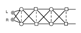
Figure 13: TBA for the susy version of the massless flow into the random bond Ising model.

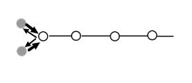
Figure 14: TBA for the susy version of the massless flow into the random bond Ising model: an equivalent form after folding.

Let us write the TBA explicitely. We give to the two grey nodes labels $0,\bar{0}$, and to the other nodes labels $1,2,\ldots$. We have thus

$$\epsilon_{0}(\theta) = {M\over 2}e^{\theta}-2Ts\star\ln\left(1+e^{-\epsilon_{1}/T}\right)$$

$$\epsilon_{\bar{0}}(\theta) = {M\over 2}e^{-\theta}-2Ts\star\ln\left(1+e^{-\epsilon_{1}/T}\right)$$

$$\epsilon_{1} = -Ts\star\left[\ln\left(1+e^{-\epsilon_{0}/T}\right)+\ln\left(1+e^{-\epsilon_{\bar{0}}/T}\right)+\ln\left(1+e^{-\epsilon_{2}/T}\right)\right]$$

$$\epsilon_{2} = -Ts\star\left[\ln\left(1+e^{-\epsilon_{1}/T}\right)+\ln\left(1+e^{-\epsilon_{3}/T}\right)+\ldots\right]$$ (106)

and

$${F\over L}=-{1\over 2\pi}\int{M\over 2}e^{\theta}\ln\left(1+e^{-\epsilon_{0}/T}\right)+{M\over 2}e^{-\theta}\ln\left(1+e^{-\epsilon_{\bar{0}}/T}\right)$$ (107)

where $s={1\over 2\pi\cosh\theta}$ and $\star$ denotes convolution.

This is quite similar to the TBA for the $O(3)$ sigma model at $\Theta=\pi$; in fact, the only difference is some factors of two in the coupling to the source nodes.

The game now consists in solving these equations numerically (after some truncation) and studying the IR limit. This is a long technical story delineated in the appendix. The main conclusion is that the TBA develops a singularity at some value of $M/T$, and that this value is very large, and probably infinite. Such intriguing behavior was studied in [42] for instance, where it was interpreted as a sign that the theory one is trying to define encounters some sort of phase transition. For the examples discussed in [42], the singularity remained at a finite value of $M/T$, so the vicinity of the IR fixed point at least was well defined. In our case, it seems the singularity might occur right near the IR fixed point, so the WZW theory sits on the border of a domain of instability in the massless region. Meanwhile, we have found that adding a CDD factor in the LR scattering seems to give a meaningful TBA, provided one chooses

$$f=\tanh^{2}(\theta/2+i\pi/4)$$ (108)

Note that this factor has a double pole at $\theta=i/2$, which leads to a ‘monstron’ with complex mass

$$M_{m}=Me^{i\pi/4}$$ (109)

similar to the one encountered in the study of the massless flow from dilute to dense polymers [43, 37]. The TBA now gives $c_{\hbox{eff}}=1$ in the UV, but it is not clear whether one should add to it a monstron contribution [44],[37]. We hope to present a more detailed study of this question elsewhere.

9 Conclusion

On the positive side, we have, in this paper:

• built the basic TBA for $OSp(2|2)$ symmetric integrable models

• found evidence that the S matrix of [12] for the GN model is the correct one

• uncovered an intriguing duality between different quantum field theories, somewhat generalizing to the massive case the results from [5, 6]

• uncovered yet another duality between the (q-deformation of) the $OSp(2|2)$ sigma model and some integrable two bosons theories

• shown that the proposal of [39] for the flow into the random bond Ising model is not correct

We have also uncovered some troubling features that seem very generic. In particular

• the S matrix of the $OSp(2|2)$ sigma model appear to be a very intriguing object, where some of the usual principles might not apply. It is not known up to now, even though the TBA has been extracted from a lattice regularization. It is also not known what kind of ‘sausage deformation’ of the sigma model corresponds to the q-deformation of the lattice equations.

It also remains to see how our analysis might fit into the more general scheme recently developed in the AdS/CFT enterprise. We note in this respect that the problems discussed in this paper could a priori be tackled as well with another form of the Bethe ansatz, corresponding to choosing a different Dynkin diagram. This question was briefly alluded to in [32]. We leave this question to further study, and simply notice that the Y system for the GN model reads (setting as usual $Y=e^{-\epsilon/T}$)

$$Y_{0}(\theta-i\pi/2)Y_{0}(\theta+i\pi/2) = (1+Y_{1}(\theta))^{2}$$

$$Y_{\bar{0}}(\theta-i\pi/2)Y_{\bar{0}}(\theta+i\pi/2) = (1+Y_{1}(\theta))^{2}$$

$$Y_{1}(\theta-i\pi/2)Y_{1}(\theta+i\pi/2) = (1+Y_{0}(\theta))(1+Y_{\bar{0}})(\theta))(1+Y_{2}(\theta))$$

$$Y_{i}(\theta-i\pi/2)Y_{i}(\theta+i\pi/2) = (1+Y_{i-1}(\theta))(1+Y_{i+1})(\theta))$$ (110)

This differs from the one for the $O(3)$ model only by a power of two appearing in the first two equations. It would be most interesting to match this Y system with some of the general results uncovered recently [45, 46, 47].

We would like to end this paper with a speculation. We have identified the q-deformed $OSp(2|2)$ sigma model with a complex version of the ${\cal C}_{1}^{(1)}$ theory discussed in [38]. Now, for the real case, V. Fateev conjectures that the ${\cal C}_{1}^{(1)}$ theory is dual to the complex sinh-Gordon model (CSG). Extending (maybe too naively) his conjecture to the complex case, we find that our q-deformed $OSp(2|2)$ sigma model should be equivalent to the complex sine-Gordon model with action

$$A={1\over 2}\int{\partial_{\mu}\chi\partial_{\mu}\bar{\chi}\over 1-{\pi^{2}\over\pi-\gamma}|\chi|^{2}}-m_{0}^{2}|\chi|^{2}+\hbox{ counterterms}$$ (111)

In particular, we obtain that the pure $OSp(2|2)$ case should correspond to

$$A={1\over 2}\int{\partial_{\mu}\chi\partial_{\mu}\bar{\chi}\over 1-\pi|\chi|^{2}}-m_{0}^{2}|\chi|^{2}+\hbox{ counterterms}$$ (112)

Of course, the coupling is now so big in the CSG that it is not clear what the action means. Yet, another important observation in favor of this proposal concerns conserved quantities. It is well known that the CSG model admits independent conserved quantities of arbitrary spin [48]. On the other hand, the S matrix encodes conserved quantities [49]; for instance, expanding the sine-Gordon S matrix (104), the poles at $k=(2n+1)i\pi$ correspond to the local conserved quantities, which act as $e^{(2n+1)\theta}$ on particles, and thus are present only for odd spin. Meanwhile, in the conjectured S matrix (103), there are poles at all $k=n\pi$, leading also to conserved quantities acting as $e^{2n\theta}$. These poles disappear in the product $Z_{I,I}Z_{I,II}$ but are otherwise present, as would be required for the CSG.

Interestingly, the question of S matrices for the complex sine-Gordon model is far from being settled [50, 51]. Our results provide an intriguing light on this question, indicating a spectrum quite different from the semi classical proposals. We will discuss this issue in more details elsewhere.

Acknowledgments: we thank A. Babichenko, D. Bernard, C. Candu, V. Fateev A. Leclair, S. Lukyanov, G. Mussardo, N. Dorey, N. Read and V. Schomerus for discussions. We also thank F. Essler, H. Frahm, I. Ikhlef and J. Jacobsen for earlier collaboration on related matters. One of the authors (B.P.) acknowledges support by the ESF INSTANS Exchange Grant (ref. number: 1799) and also by the Hungarian OTKA grants K75172 and K60040. The other author acknowledges support from the Agence Nationale pour la Recherche.

Appendix A: Numerical study of the massless TBA

A.1 $O(3)$ sigma-model with $\theta=\pi$: a reminder

We first consider this case as a warmup. The infinite set of TBA equations is well known (see also Fig. 15):

$$\begin{split}\epsilon_{0}&=re^{\theta}/2-s\star\ln\big{(}1+e^{-\epsilon_{1}}\big{)}\\ \epsilon_{\bar{0}}&=re^{-\theta}/2-s\star\ln\big{(}1+e^{-\epsilon_{1}}\big{)}\\ \epsilon_{1}&=-s\star\ln\big{(}1+e^{-\epsilon_{0}}\big{)}-s\star\ln\big{(}1+e^{-\epsilon_{\bar{0}}}\big{)}-s\star\ln\big{(}1+e^{-\epsilon_{2}}\big{)}\\ \epsilon_{i}&=-s\star\ln\big{(}1+e^{-\epsilon_{i-1}}\big{)}-s\star\ln\big{(}1+e^{-\epsilon_{i+1}}\big{)}\quad\text{for}\quad i=2,3,\dots\end{split}$$ (A1)

with $s=\frac{1}{2\pi\cosh{\theta}}$, we have rescaled the $\epsilon$’s with respect to the main text, and set $r=M/T$.

The dimensionless free energy per unit length $F(r)$ is calculated as

$$F=-\frac{1}{2\pi}\int\frac{e^{\beta}}{2}\ln\big{(}1+e^{-\epsilon_{0}}\big{)}+\frac{e^{-\beta}}{2}\ln\big{(}1+e^{-\epsilon_{\bar{0}}}\big{)}$$

In the UV and IR limit it is related to the central charge as $F=-c/12$.

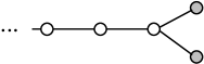
Figure 15: TBA for the $O(3)$ sigma-model with $\theta=\pi$

The above set of equations has to be truncated to be accesible to numerical investigations. Let us denote the total number of nodes with $N$. The expected values of the central charge are

$$c_{UV}=2-\frac{6}{N+2}\quad\quad\quad\quad c_{IR}=1-\frac{6}{(N+2)(N+3)}$$

The function $F(r)$ is plotted for two different values of $N$ in Fig. 16.

\psfrag{cinIR}{$c_{IR}$}\psfrag{cinUV}{$c_{UV}$}\psfrag{log10r}{$\log r$}\psfrag{F}{$F$}\includegraphics{sN6.eps}

(a) $N=6$

\psfrag{cinIR}{$c_{IR}$}\psfrag{cinUV}{$c_{UV}$}\psfrag{log10r}{$\log r$}\psfrag{F}{$F$}\includegraphics{sN10.eps}

(b) $N=10$

Figure 16: $F(r)$ in the truncated versions of the $\sigma$-model TBA

Convergence as a function of $N$ is clearly rather quick. To see this better, consider $F$ as a function of $N$ for different fixed values of $r$. The results for $r=0.1,1,10$ are shown in Fig. 17. One can see that there is a well-defined $N\to\infty$ limit, the leading correction is $O(1/N)$.

\psfrag{r0.1}{\small$r=0.1$}\psfrag{rii1}{\small$r=1$}\psfrag{ri10}{\small$r=10$}\includegraphics{F_of_N_sigma.eps}

Figure 17: $F$ as a function of $N$ for $r=0.1,1,10$ in the $O(3)$ sigma-model with $\theta=\pi$

A.2 The conjectured massless flow in the $OSP(2|2)$ case

The infinite set of TBA equations given in the text becomes:

$$\begin{split}\epsilon_{0}&=re^{\theta}/2-2s\star\ln\big{(}1+e^{-\epsilon_{1}}\big{)}\\ \epsilon_{\bar{0}}&=re^{-\theta}/2-2s\star\ln\big{(}1+e^{-\epsilon_{1}}\big{)}\\ \epsilon_{1}&=-s\star\ln\big{(}1+e^{-\epsilon_{0}}\big{)}-s\star\ln\big{(}1+e^{-\epsilon_{\bar{0}}}\big{)}-s\star\ln\big{(}1+e^{-\epsilon_{2}}\big{)}\\ \epsilon_{i}&=-s\star\ln\big{(}1+e^{-\epsilon_{i-1}}\big{)}-s\star\ln\big{(}1+e^{-\epsilon_{i+1}}\big{)}\quad\text{for}\quad i=2,3,\dots\end{split}$$ (A2)

with $s=\frac{1}{2\pi\cosh{\theta}}$. The only difference compared to the case of the $\sigma$-model is a factor of 2 in the equations for $\epsilon_{0}$ and $\epsilon_{\bar{0}}$. However, this factor dramatically changes the behaviour of the TBA. Similar to the $\sigma$-model, we first study the truncated systems with $N$ nodes.

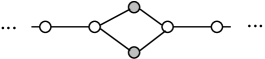
Figure 18: TBA for the susy version of the massless flow into the random bond Ising model: an equivalent form after folding.

The unfolded version of the TBA is represented by the graph in fig. 18, which only contains simple links. Given this structure of the TBA, only those diagrams can describe a meaningful flow for which the largest eigenvalue $\lambda_{\text{m}ax}$ of the incidence matrix is less than 2 [54]. If this condition is satisfied, in the UV limit one observes the usual pattern of plateus in the functions $L_{i}=\log(1+e^{-\epsilon_{i}})$ in the central region $|\theta|<\log r$. On the other hand, if $\lambda_{\text{m}ax}>2$, then one expects divergences in the UV limit . This is the case for the diagram 18, even for finite $N$. Nevertheless the calculation for the central charge is well-defined in the IR and leads to

$$c_{IR}=3-3\frac{3N-1}{N(N+1)}$$

We performed numerical calculations for different values of $N$, the results for $N=6$ and $N=10$ are shown in Fig. 19. One observes that the truncated equations work fine in the IR and produce the predicted central charges. However, the iterations become unstable (the pseudoenergies and also $F$ diverge to minus infinity) whenever $r$ is below some critical ($N$-dependent) value. One finds moreover that $r_{crit}$ increases with $N$.

\psfrag{cinIR}{$c_{IR}$}\includegraphics{N6.eps}

(a) $N=6$

\psfrag{cinIR}{$c_{IR}$}\includegraphics{N10.eps}

(b) $N=10$

Figure 19: $F(r)$ in the truncated version of the massless TBA (A2). The dashed line corresponds to the analytical prediction in the IR. The filled circles show the critical values of $r$ where the TBA equations become unstable.

We determined $r_{crit}$ for different values of $N$, the results are shown in Table 1. and Fig. 20. The numerical iterations become more time demanding as $N$ is increased, therefore we had to content ourselves with an accuracy of $\Delta r=0.1$ for the larger values of $N$.

$N$	$r_{crit}$
4	0.32175
6	1.305
8	2.016
12	2.95
20	4.1
30	4.7
50	5.5

Table 1: $r_{crit}$ for some values of $N$

\psfrag{rcrit}{$r_{crit}$}\includegraphics{critical_r.eps}

Figure 20: Critical value of $r$ as a function of $N$

At this point it is not clear what happens with $r_{crit}$ as $N$ is increased further. There are two possibilities:

1. There exists a limiting value for $r_{crit}$ as $N\to\infty$. In this case the infinite set of TBA equations would be meaningful in the interval $r=r_{crit}\dots\infty$. However, one would see unusually high effective central charges, since already for $N=20$ and $r=4$ one has $c_{eff}\approx 10$.

2. $r_{crit}\to\infty$ as $N\to\infty$.

To gain more insight, one can consider $F$ as a function of $N$ for different fixed values of $r$; the results are shown in Fig. 21. For $r\leq 5$ we observed, that the iterations become unstable whenever $N$ reaches a critical value $N_{c}<100$. These points are marked with solid squares in the figure. For $r>5$ we did not find the critical values of $N$, because we had to restrict the calculations to $N<100$. However, from the figure it is clear that even for $r>5$ there is no convergence. In fact one observes a linear gorwth in $N$ for every value of $r$, suggesting that even for $r>5$ there always exists a (possibly quite large) critical $N$. This means in turn, that in the $N\to\infty$ limit one has $r_{crit}\to\infty$.

Figure 21: $F$ as a function of $N$ for different fixed values of $r$. The solid square represent the critical values of $N$, where the iterations become unstable.

We tried the improve the TBA by introducing alternative truncation schemes for the infinite diagram, for example putting a “fork” at the end. However, none of these tricks works to stabilize the iterations for small $r$, because $\lambda_{\text{m}ax}$ will still be greater than 2.

Based on the evidence presented above, we conclude that the infinite set of equations (A2) cannot be solved for any finite $r$.

Appendix B: Modifications of the massless TBA

B.1 CDD-factors

It is a natural idea to add CDD factors to the conjectured S-matrix and to consider the resulting TBA equations. CDD factors in the LL and RR channels would alter the IR central charge, and therefore we can exclude them. The only possibility is to introduce CDD factors for $S_{RL}$ and $S_{LR}$.

A simple factor of

$$f_{\alpha}=\frac{\sinh\theta-i\sin\alpha\pi}{\sinh\theta+i\sin\alpha\pi}$$

introduces a coupling between the massless nodes in the TBA equations

$$\begin{split}\epsilon_{0}&=re^{\theta}/2-2s\star\ln\big{(}1+e^{-\epsilon_{1}}\big{)}-\varphi_{\alpha}\star\ln\big{(}1+e^{-\epsilon_{\bar{0}}}\big{)}\\ \epsilon_{\bar{0}}&=re^{-\theta}/2-2s\star\ln\big{(}1+e^{-\epsilon_{1}}\big{)}-\varphi_{\alpha}\star\ln\big{(}1+e^{-\epsilon_{0}}\big{)}\\ \epsilon_{1}&=-s\star\ln\big{(}1+e^{-\epsilon_{0}}\big{)}-s\star\ln\big{(}1+e^{-\epsilon_{\bar{0}}}\big{)}-s\star\ln\big{(}1+e^{-\epsilon_{2}}\big{)}\\ \epsilon_{i}&-s\star\ln\big{(}1+e^{-\epsilon_{i-1}}\big{)}-s\star\ln\big{(}1+e^{-\epsilon_{i+1}}\big{)}\quad\text{for}\quad i=2,3,\dots\end{split}$$ (B1)

where

$$\varphi_{\alpha}=\frac{1}{2\pi}\frac{2\cosh\theta\sin\alpha\pi}{\sinh\theta^{2}+\sin^{2}\alpha\pi}$$

The function $\varphi_{\alpha}$ has the same sign as $s=\frac{1}{2\pi\cosh\theta}$ if $\alpha>0$, therefore it makes the situation even worse. The only possibility to ”cure” the TBA is to choose $\alpha<0$. In this case there is a pole in the physical sheet at $\theta=i\alpha$, which should be explained. However, the TBA makes sense perfectly, irrespective of the value of $\alpha$. In fact, $\alpha$ can be chosen arbitrarily, because it only determines the crossover scale $M$. Choosing $\alpha=1/2$ one obtains

$$f=\tanh^{2}(\theta/2+i\pi/4)\qquad\text{with}\qquad\varphi=-\frac{1}{\pi\cosh\theta}$$

The folded version of the TBA is then represented by the graph below, where the vertical line with the arrows represents ,,negative” coupling.

The UV central charge cannot be obtained in the usual way, because there are still no finite plateus in $L=\log(1+e^{-\epsilon})$ and in the central region one has $\epsilon_{i}=-\infty$ for every node. Instead one can consider the truncated diagrams with $N$ nodes and let $N\to\infty$. This way one obtains

$$c_{\hbox{eff}}=1\quad\text{(UV)}\qquad\qquad c_{\hbox{eff}}=3\quad\text{(IR)}$$

The above results were obtained by numerically solving the Y-system equations

$$\begin{split}Y_{0}(\theta-i\pi/2)Y_{0}(\theta+i\pi/2)&=(1+Y_{1}(\theta))^{2}\frac{1}{(1+Y_{\bar{0}}(\theta))^{2}}\\ Y_{\bar{0}}(\theta-i\pi/2)Y_{\bar{0}}(\theta+i\pi/2)&=(1+Y_{1}(\theta))^{2}\frac{1}{(1+Y_{0}(\theta))^{2}}\\ Y_{1}(\theta-i\pi/2)Y_{1}(\theta+i\pi/2)&=(1+Y_{0}(\theta))(1+Y_{\bar{0}}(\theta))(1+Y_{2}(\theta))\\ Y_{i}(\theta-i\pi/2)Y_{i}(\theta+i\pi/2)&=(1+Y_{i-1}(\theta))(1+Y_{i+1}(\theta))\end{split}$$ (B2)

with constant numbers $y_{i}$ and evaluating the central charge with the usual rules. We do not know of an exact analytical proof. However, we can give an approximate solution, as follows.

Let us consider a truncated diagram with $N$ nodes denoted by $0,\bar{0},1,\dots(N-2)$. In the UV limit the variables $y_{i}=e^{-\epsilon_{i}}$ take the values

$$y_{0}=y_{\bar{0}}\approx\sqrt{\frac{27(N-2)^{2}}{4\pi^{2}}}\qquad\qquad y_{i}\approx\frac{9(N-2)^{2}}{2\pi^{2}}\left(1-\cos\left(\frac{2\pi(N-2-i)}{3(N-2)}\right)\right)$$ (B3)

in the central region. On the other hand, for $\theta\to\infty$ the constant values are approximately

$$y_{0}=0\qquad y_{\bar{0}}\approx\frac{4(N-2)^{2}}{\pi^{2}}\qquad y_{i}\approx\frac{2(N-2)^{2}}{\pi^{2}}\left(1-\cos\left(\frac{\pi(N-2-i)}{N-2}\right)\right)$$ (B4)

Actually, in this latter case the exact solution is known, because this corresponds to the Y-system equations of the $A_{n}$ diagram with $n=2N-3$. However, the exact solution is not needed. The effective central charge only depends on the way the variables $y_{i}$ approach infinity for $N\to\infty$ in (B3) and (B4). Substituting the above values into eq. (5.3) of [54] yields $c=1$ in the $N\to\infty$ limit.

We performed numerical simulations of the truncated equations (B1) with different values of $N$ between $N=10$ and $N=40$ and extrapolated the results to $N\to\infty$ applying a polynomial fit in $1/N$. The results are shown in Fig. 22.

\psfrag{log10r}{$\log_{10}r$}\psfrag{ceff}{$c_{eff}$}\includegraphics{Ninfty_CDD.eps}

Figure 22: The evolution of the effective central charge in the massless TBA with a CDD factor.

We note that a simple factor of $\tanh(\theta/2+i\pi/4)$ is not sufficient to stabilize the TBA, because in this case one still has $\lambda>2$ even for the truncated diagrams.

B.2 $S_{LR}$ being a pure CDD factor

In this case (which was in fact discussed earlier in the literature [39]) the theory posseses two independent $OSP(2|2)$ symmetries corresponding to $LL$ and $RR$ scattering.The TBA we are dealing with is now represented by the diagram

The vertical line connecting the two inifinite chains corresponds to the CDD factor. A simple factor of

$$S_{LR}=\tanh(\theta/2-i\pi/4)$$

(which proved to be the correct choice in [55] and [56]) does not work in this case, because once again the TBA will be oversaturated. The simplest possibility is to choose the inverse of the latter:

$$S_{LR}=\tanh(\theta/2+i\pi/4)$$

In this case the dashed link corresponds to

$$\varphi=-\frac{1}{2\pi\cosh\theta}$$

The TBA now gives $c_{eff}=0$ in the UV (the truncated diagrams have finite positive $c_{eff}$, which tends to zero if $N\to\infty$), which is a probably meaningless result.

References

- [1] H. Saleur and B. Wehefritz-Kaufmann, Nucl. Phys. B628. (2002) 407.
- [2] Z. Tsuboi, Phys.Lett. B544 (2002) 222.
- [3] B. Wehefritz Kaufmann and H. Saleur, Nucl.Phys. B663 (2003) 443.
- [4] N. Mann and J. Polchinski, Phys.Rev.D72:086002,2005; hep-th/0508232.
- [5] C. Candu and H. Saleur, N ucl. Phys. B808 (2009) 487.
- [6] V. Mitev, T. Quella and V. Schomerus, JHEP 0811:086,2008.
- [7] H. Saleur and V. Schomerus, Nucl.Phys.B775:312-340,2007.
- [8] F. Essler, H. Frahm and H. Saleur, Nucl.Phys. B712 (2005) 513.
- [9] W. Galleas and M.J. Martins, Nucl.Phys.B768 (2007) 219; hep-th/0612281.
- [10] A.B. Zamolodchikov and Al. B. Zamolodchikov, Ann. Phys. 120 (1979) 253.
- [11] M. Karowski and H.J. Thun, Nucl. Phys. B190 (1981) 61.
- [12] Z. Bassi and A. Leclair, Nucl. Phys. B578 (2000) 577; hep-th/9911105
- [13] M.P. Pfannm ller and H. Frahm, J. Phys. A 30 (1997) L543.
- [14] J. Balog, S. Naik, F. Niedermayer and P. Weisz, Phys. Rev. Lett. 69 (1992) 873.
- [15] D. Arnaudon, J. Avan, N. Crampé, A. Doikou, L. Frappat and E. Ragoucy, Nucl.Phys. B687 (2004) 257.
- [16] P. Kulish, N. Reshetikhin, and E. Sklyanin, Lett. Math. Phys. 5(1981) 393; L. Takhtajan, Phys. Lett. 90A (1982) 479 ; H. Babujan, Phys. Lett. 93A (1982) 464.
- [17] H. Saleur and B. Wehefritz-Kaufmann, Phys.Lett. B481 (2000) 419.
- [18] J.L. Jacobsen and H. Saleur, Nucl. Phys. B743 (2006) 207.
- [19] P. Fendley and K. Intrilligator, Nucl.Phys. B372 (1992) 533 ; Nucl.Phys. B380 (1992) 265
- [20] A. B. Zamolodchikov and Al. B. Zamolodchikov, Nucl. Phys. B379 (1992) 602.
- [21] A. B. Zamolodchikov, Nucl. Phys. B366 (1991) 122.
- [22] V. Fateev, Phys. Lett. B324 (1994) 45.
- [23] P. Hasenfratz, M. Maggiore and F. Niedermayer, Phys. Lett. B245 (1990) 522.
- [24] I. Bars and R. Kallosh, Phys. Lett. B233 (1989) 117.
- [25] N. Yu Reshetikhin and H. Saleur, Nucl. Phys. B419 (194) 507.
- [26] C. Destri and H. de Vega, Nucl. Phys. B438 (1995) 413.
- [27] A. Hegedus, Nucl.Phys. B679 (2004) 545; hep-th/0310051.
- [28] R. Shankar, Phys. Rev. Lett. 55, (1985) 453.
- [29] V. E. Korepin, Theo. Math. Phys. , 41:2 (1979), 169; N. Andrei and C. Destri, Nucl. Phys. B231 (1984) 445.
- [30] Al. Zamolodchikov, Int.J.Mod. Phys., A10 (1995) 115
- [31] M. Bocquet, D. Serban, M. Zirnbauer, Nucl. Phys. B 578 (2000) 628.
- [32] J.L. Jacobsen and H. Saleur, Nucl. Phys. B716 (2005) 439.
- [33] A. Strominger and T. Takayanagi, Adv. Theor. Math. Phys. 7 (2003) 369
- [34] S. Fredenhagen and V. Schomerus, hep-th/0308205.
- [35] Z. Maassarani, J.Phys. A28 (1995) 1305.
- [36] P. Fendley and H. Saleur, Nucl. Phys. B388 (1992) 609.
- [37] Al. B. Zamolodchikov, Phys. Lett. B335 (1994) 436.
- [38] V. Fateev, Nucl. Phys. B479 (1996) 594. See eq. (1) with , in this reference.
- [39] D.C. Cabra, A. Honecker, G. Mussardo and P. Pujol, J.Phys.A30 (1997) 8415.
- [40] P. Fendley, Phys.Rev. B63 (2001) 104429; cond-mat/0008372
- [41] D. Bernard, ‘(Perturbed) Conformal Field Theory Applied To 2D Disordered Systems: An Introduction’, hep-th/9509137.
- [42] G. Mussardo and P. Simon, Nucl.Phys. B578 (2000) 527.
- [43] P. Fendley, H. Saleur and A. Zamolodchikov, Int. J. Mod. Phys. A8 (1993) 5717.
- [44] P. Dorey, A. Pocklington and R. Tateo, Nucl.Phys. B661 (2003) 464; hep-th/0208202
- [45] Z. Tsuboi, “Solutions of the T-system and Baxter equations for supersymmetric spin chains”, arXiv:0906.2039
- [46] V. Kazakov, A. Sorin and A. Zabrodin, Nucl.Phys.B790 (2008) 345; hep-th/0703147.
- [47] V. Kazakov and P. Vieira, JHEP10:050,200; arXiv: 0711.2470.
- [48] I. Bakas, Int. J. Mod. Phys. A9 (1994) 3443.
- [49] M. Niedermaier, Nucl. Phys. B424 (1994) 184.
- [50] N. Dorey and T. J. Hollowood, Nucl. Phys., B440 (1995) 215; hep-th/9410140.
- [51] J.L. Miramontes, Nucl. Phys. B702 (2004) 419.
- [52] G. Feverati, F. Ravanini and G. Takacs, Nucl.Phys. B570 (2000) 615; hep-th/9909031
- [53] C. Ahn and A. Babichenko, “TBA analysis of invariant integrable model”, unpublished.
- [54] F. Ravanini, R. Tateo and A. Valleriani, Int.J.Mod.Phys. A8 (1993) 1707.
- [55] Al. B. Zamolodchikov, Nucl. Phys. B358 (1991) 524.
- [56] A. B. Zamolodchikov and Al. B. Zamolodchikov, Nucl. Phys. B379 (1992) 602.