Reducing multi-dimensional information into a 1-d histogram

Abstract

We present two methods for reducing multidimensional information to one dimension for ease of understand or analysis while maintaining statistical power. While not new, dimensional reduction is not greatly used in high-energy physics and has applications whenever there is a distinctive feature (for instance, a mass peak) in one variable but when signal purity depends on others; so in practice in most of the areas of physics analysis. While both methods presented here assume knowledge of the background, they differ in the fact that only one of the methods uses a model for the signal, trading some increase in statistical power for this model dependence.

1 Introduction

Statistical analysis in high-energy physics is a complex field, with many multi-dimensional analysis techniques used by the various experiments. The uncomfortable truth remains that while the visualisation and especially comparison of one dimensional information is relatively straightforward, two dimensional graphs are already extremely difficult to compare in a meaningful manner and higher dimensional distributions are essentially impossible. We therefore present two techniques intended to simplify that comparison, showing alternative versions of the projection into the relevant variable, both of which keep most of the statistical power of the other hidden ones. The basic ideas are not new[2, 1], but they have not been much used in high-energy physics.

Both techniques allow for fits etc. to be performed in one dimension, with the advantages of visibility of the fitting function and the background distribution, and therefore easier handling of the systematics. They thus partially undo the ‘curse of dimensionality’[3].

This paper is divided into different sections. The first (section 2) introduces an example distribution which is considered throughout this note. Section 3 discusses the first method, that consists in collapsing a multi-dimensional distribution into a 1-dimensional one, making only assumptions on the background. This method can provide a model-independent search for effects like mass peaks above a Standard Model background assumed to be known. It can also be used when signal model is uncertain and minimal assumptions are to be made.

The technique shown in section 4 also uses a weighting technique to reduce a multidimensional distribution into a one dimensional one, but this time having as an input also the expected signal density, such that for un-correlated variables (almost) the full statistical power is available in the one-dimensional distribution. Furthermore the use of approximate multi-dimensional distributions will lead to a decrease in the statistical power, and not to false discoveries.

2 Example search problem

In order to compare the different methods we introduce an example distribution. We chose to consider the simplest case of the reduction of a 2-dimensional distribution into 1D, as in this case the full information can be shown graphically, but the techniques extend trivially into higher dimensions. The example chosen is a Gaussian signal in one dimension, decaying exponentially in the other dimension, while the background is flat in the first dimension and exponentially falling (sharper than the signal) in the second one:

$$\sigma_{back} = e^{p_{T}/30}$$ (1)

$$\sigma_{sig} = e^{p_{T}/80}\cdot e^{-0.5((m-91)/3)^{2}}$$ (2)

This kind of behaviour may arise, for instance, in the search for a new particle where the mass and p_T of candidate objects are measured, and an excess is expected to have a particular mass plus a harder p_T distribution than the background. The distribution can be seen in Figure 1.

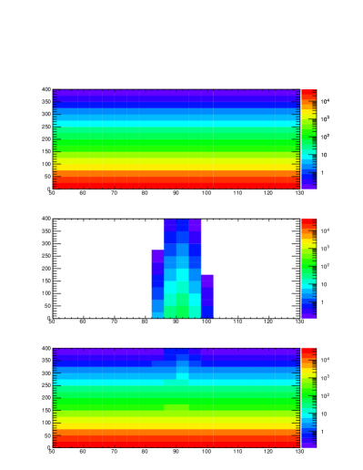
Figure 1: The distribution in mass and $p_{\mathrm{T}}$ space of the background (top), the signal (centre) and the total (bottom).

3 Signal model-independent dimensional reduction

Let’s start by considering the case where we assume we know the distribution of background, and we want to look for an excess in the data. We want to reduce the initial N-dimensional distribution into a single histogram, that keeps the same statistical power as the initial distribution. We define two N-dimensional histograms, for data and for the expected background, called $D_{i,j,...p}$ and $B_{i,j,...p}$ and assume for simplicity that we want to project them into the first dimension, denoted by the letter i. The problem can be seen as finding for each bin $i^{\prime}$ of the distribution along the first variable two values of signal and background that have the same $\chi^{2}$ probability as the combination of all the other bins with the first variable in bin $i^{\prime}$. In practice, for all bins with the first variable in $i^{\prime}$, we calculate the low-statistics Poisson approximation[4] value of

$$\chi^{2}=2(B_{i,j,...p}-D_{i,j,...p})+2D_{i,j,...p}ln(D_{i,j,...p}/B_{i,j,...p})$$

and sum these values over all the dimensions to collapse. We also calculate a signed $\chi^{2}_{sign}$ distribution, made of a sum the same terms as before, but with the minus sign for the bins where the number of data events is smaller than the background expectation.

Then we take the probability P to have the total value of the unsigned $\chi^{2}$ for the appropriate number of degrees of freedom. Since we want the final 1-dimensional histogram not to distort the observation from data, we assign the number of data events for the bin $i^{\prime}$ to be the total number of events observed there, i.e. the projection over all other dimensions, with no further manipulation. For background, if we want to keep the same statistical significance of the multi-dimensional distribution, we clearly cannot just sum over the other variables. Instead, we calculate the value of $\chi^{2}$ that would yield the probability P for one degree of freedom. Using the above expression, and given the number of observed data events, there are two solution for the number of background events, one larger and the other smaller than the number of data events. We select the first solution if $\chi^{2}_{sign}>0$, the second otherwise, in order to properly account for under-fluctuations in data.

4 Signal model-dependent dimensional reduction

The previous section discussed reduction of a multidimensional space into a one dimensional one without making any assumption on the distribution of signal, so it suits general search problems. The technique here, in contrast, will assume a signal distribution, and is more suited to the case when a model for the search signal is available.

Similarly to the previous case, the idea is to collapse N variables into a single one, this time using weights that would optimise the separation between a known signal and background.

4.1 Calculation of optimal weighting

Take the example of a search with two bins, with expected background $b_{i}$ and signal $s_{i}$, and with Gaussian distributed errors on the bins $\delta_{i}$ so that they each have an expected significance $\sigma_{i}=s_{i}/\delta_{i}$. If we combine them into one bin, applying weights $w_{i}$ to each of them as we do so, then the combined total is

$$b_{T} = W_{1}b_{1}+W_{2}b_{2}$$ (3)

$$s_{T} = W_{1}s_{1}+W_{2}s_{2}$$

$$\delta_{T}^{2} = (W_{1}\delta_{1})^{2}+(W_{2}\delta_{2})^{2}$$

$$\sigma_{T}^{2} = \frac{(W_{1}s_{1}+W_{2}s_{2})^{2}}{(W_{1}\sigma_{1})^{2}+(W_{2}\sigma_{2})^{2}}$$

The total significance is maximised if we use:

$$\frac{W_{2}}{W_{1}} = \frac{\sigma_{1}^{2}}{s_{1}}\frac{s_{2}}{\sigma_{2}^{2}}$$ (4)

We can set $W_{1}$ arbitrarily, as the weights are relative. If we choose $W_{1}=s_{1}/\sigma_{1}^{2}$ then we see $W_{2}=s_{2}/\sigma_{2}^{2}$. Given an arbitrary number of bins, and considering merging them sequentially pairwise, we see that this weight function is optimal for any number of bins. There remains however an arbitrary scale; in this note we scale all weights so that the largest weight in any bin is 1 in all cases.

There is an implicit assumption that the errors are Gaussian. Note that at this level this only effects the optimality or otherwise of the combination. If we assume that errors are of the form $\delta_{i}=\sqrt{b_{i}}$ then the optimal weight is $W_{i}=s_{i}/b_{i}$; an alternative assumption is $\delta_{i}=\sqrt{s_{i}+b_{i}}$, leading to $W_{i}=s_{i}/(s_{i}+b_{i})$. However, if the entire result is to be represented in a single one-dimensional plot, which is the aim, then the errors on the final combined bin must have a Gaussian form. This in turn requires that the effective number of events, $(\Sigma_{i}w_{i})^{2}/\Sigma_{i}w_{i}^{2}$, in each bin must be large.

The question of how to find the signal and background densities to calculate these weights is not addressed here. However, it must be stressed that an incorrect weight produces a non-optimal result, and not an incorrect one, and therefore an approximate method such as the matrix element technique or ignoring correlations between variables can legitimately be applied. The weighting treatment is being applied as a procedure to the data but all interpretation is reserved for the final distribution.

5 Application to the example problem

The problem introduced in section 2 is used here. The $p_{\mathrm{T}}$ spectra of signal and background are shown in figure 2. These functions are perfectly known, and used both to create distributions and to fit them.

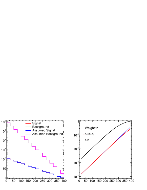
Figure 2: The $p_{\mathrm{T}}$ spectra. Top is the actual spectra used, bottom is the shapes of different possible weight functions. Shown in black is the one adopted; the straight blue line shows $s/b$ and $s/(s+b)$ is in red.

In the signal weighting reduction method the distinction between $s/b$ and $s/(s+b)$ errors needs discussion. The derivation assumed errors on the input bins were all Gaussian, but in multidimensional distributions this is unlikely to be correct. The choice of $s/(s+b)$ provides an upper cut-off on the weight function which serves to regulate the distribution of weights. This allows application of the central limit theorem to the sum of the weights to calculate the error on the resulting bins.

As has been stressed, it is a subjective decision how one builds these weights. For example, the background and signal strengths entering in these formula ignore the final dimension (in this case, mass). Thus the background strength actually affecting the analysis on the mass peak is much smaller than is estimated from the other variables. To reflect this the background strength parameter used to calculate the weight is reduced by width of the signal divided by the width of the total distribution.

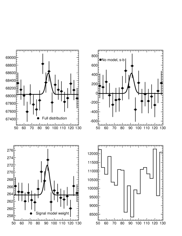
Figure 3: The mass spectra. Top left is all the events projected onto the mass axis. Top right shows the background-subtracted no-model projection. The bottom plots are the signal model weight projected version on the left and the corresponding effective number of events per bin on the right. This is a sample distribution for one trial.

The mass distributions appear as figure 3. The total projection (top left) has a very poor significance, and it is hard by eye to see any signal. The model-independent approach results in a final distribution (after background is subtracted from the signal) shown on the top right, with a peak which is more apparent. The weighted sum, however, (bottom left) also has a distinctly clearer picture. It will also be seen that it is statistically better distinguished as well. The distribution of the effective number of events (bottom right) is useful to check that a sufficiently large number of events is used, to justifying the use of the central limit theorem.

Four different approaches to the analysis are compared. The first is a fit to the full 2D distribution, an the other three are one one dimensional projections obtained simply by varying a cut or with the reduction methods discussed. In each case there are two free parameters: the signal level and the background level.

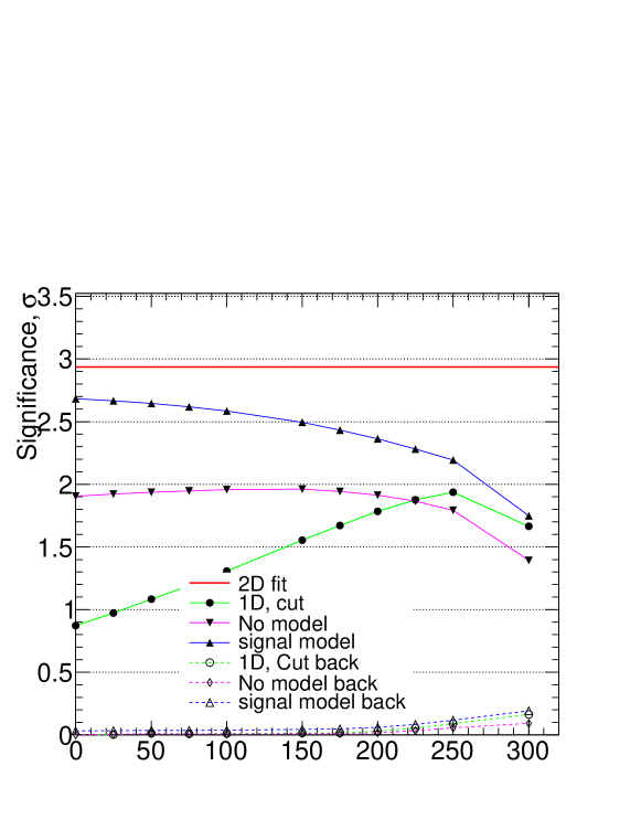
Figure 4: The mean significance over many trials reported by each analysis as a cut on the $p_{\mathrm{T}}$ is varied. In the case of the 2d fit, the cut was not applied and a fixed line is shown. Also shown, dashed, are the mean significances reported when fits are made to background only distributions. This climbs above zero when a $\chi^{2}$ approximation is used with insufficient events.

The statistical power of the various analysis methods is investigated in figure 4. For the three analyses where the final extraction is done with a $\chi^{2}$ fit in 1D with the signal and background size as free parameters. What is plotted is the claimed significance of the signal. For the 2D case a likelihood analysis is used as some bins have low numbers of events. The fit occasionally failed to converge, and so the signal size has been fixed at the expected value and what is measured is the difference in log likelihood with and without a signal. As $-2\log{\cal L}\simeq\chi^{2}$, the plot shows the mean of the signed square-root of twice the log likelihood, and it will be necessary to test how accurately this represents the number of sigmas.

The solid curves show the expected significance on signal plus background samples, while dashed is the expected significance for background only. This is not zero because the signal strength is not allowed to be negative as this causes problem in a likelihood fit.

The most powerful procedure is to make a 2D fit, as expected. The signal model weighted fit produces a performance almost equal to the 2D fit when applied to the whole distribution, gradually declining as data is cut away. The cut based analysis suffers from excessive background when all the data is considered, and rises in power as this is removed. After some point the reduction in signal becomes more important and the significance drops. Note that at this point the expected significance for the background only experiments is rising, suggesting that the Gaussian approximation is breaking down.

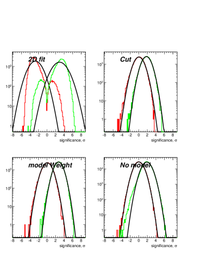
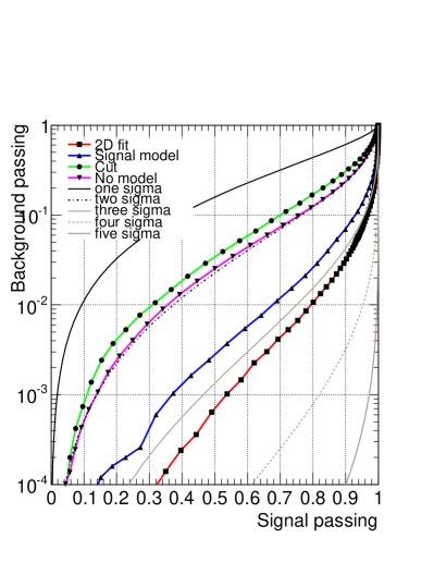
Figure 5: The actual separation power of the fits. The plot on the left shows the number of sigma reported in toy MC experiments for background only and signal plus background ensembles. The plot on the right shows the same data plotted as fractional efficiencies which could be achieved by a sliding cut. The simple cut based approach is evaluated at a 200 GeV cut, others are for the full distribution.

Figure 5 shows the power of each of the fits. The plots on the left show the significance in toy MC experiments. The four curves show reasonable agreement with the sensitivities reported by the fit means, with the only exception being the full 2D fit. The estimated mean significance was 2.9 $\sigma$, while the observed sensitivity is more like a 3.1 $\sigma$ separation. This is not surprising - the approximate connection between likelihood and $\chi^{2}$ used is conservative.

5.1 Signal biases

The model of the signal used will almost always be, in some details, imperfect. How major a problem this is depends upon the type of defect, but it will in general reduce the sensitivity to a new signal or distort the measurement of its parameters. Two biases are consider here: the first is that the dependence of cross-section on $p_{\mathrm{T}}$ has an exponential slope which is not the one expected, while the second is that there is a linear correlation between mass and $p_{\mathrm{T}}$ in the signal, which is assumed not to exist.

The slope of the signal, given in equation 2 as $e^{p_{T}/80}$ is changed to be 60, 70 100 or 200, while the 1D and 2D analysis techniques are applied, assuming a slope of 80. The results for the expected significance are shown in figure 6.

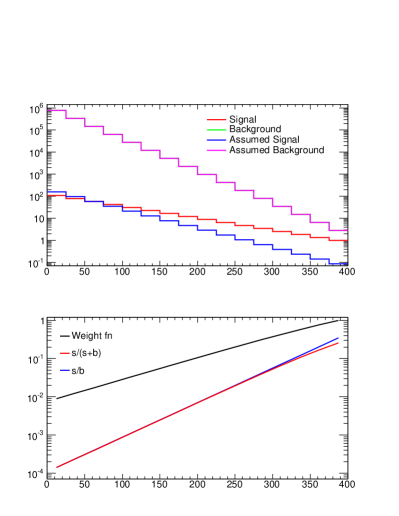
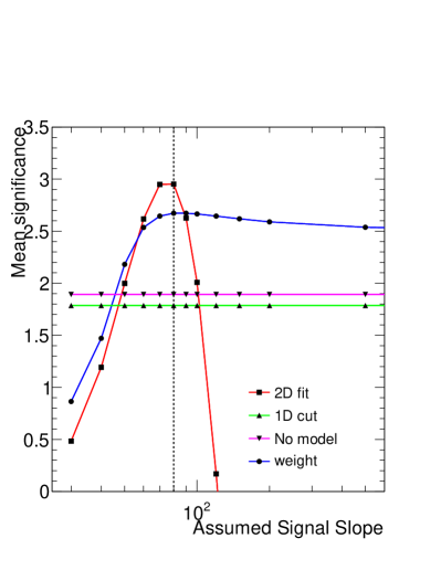
Figure 6: The effect of using the wrong slope in the analysis. The plot on the left shows an example for an assumed slope of 50. On the right is the expected significance of the various techniques when the wrong signal slope is used in the analysis. All samples have a slope of $e^{p_{T}/80}$, as marked. A large slope parameter corresponds to a flat distribution.

It can be seen that the two 2D fit performs best when the correct slope parameter is used. However, when too large or too small a slope is assumed, the power degrades. The weighted fit shows similar behaviour, with a lower peak power and a considerably reduced dependence upon the slope value so that if the slope estimate is 20% wrong or more it becomes more powerful. When the assumed slope is 30, this is the same as the background slope; at this point the weighted analysis is identical to simply ignoring any $p_{T}$ dependence. The cut analysis was not re-optimised but always used a 200 GeV $p_{T}$ cut, and therefore does not depend upon the assumed slope; in reality if the optimisation was done with the wrong slope its performance might reduce. The no-model approach has no dependence by construction.

The second bias investigated is when a correlation is inserted between the mass and the $p_{\mathrm{T}}$ of the signal, with a linear shift proportional to the $p_{\mathrm{T}}$. This means that any any particular $p_{\mathrm{T}}$ the signal width in mass is unchanged, but that averaged over $p_{\mathrm{T}}$ it is widened. The effects are shown in figure 7.

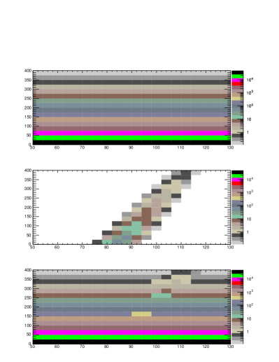
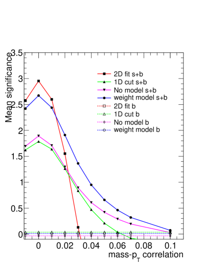
Figure 7: The effect of correlating mass and $p_{\mathrm{T}}$ in the signal. Left is the distribution when a correlation factor 0.7 is used, right is the expected significance of various techniques when the a correlations between mass and $p_{\mathrm{T}}$ is introduced in the signal but not the analysis.

This particular form of distortion means that a correct 2D fit, allowing for the slope, would not be affected. However, all the analyses loose power here, and the 2D fit is the most sensitive. This is probably because it is the highest weight events, at largest $p_{\mathrm{T}}$, which move most, thus distorting the likelihood. The signal weighting method uses weights whose distribution is truncated to obtain Gaussian errors, and this seems to protect it in this example.

5.2 Background biases

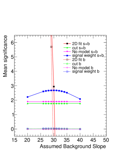
Figure 8: The effect of using the wrong background slope in the analysis. The expected significance of the various techniques is shown for background only and signal plus background samples.

Figure 8 shows the effect of using the wrong background slope on the fits. All the fits vary the background level, and for the one dimensional fits this means that there is no false discovery. For the 2D fit the slope error is interpreted as evidence for a signal. The blind application of the 2D method clearly produces absurd results.

This is a major advantage in using the 1D distributions - the analysis is done in 1D with less variables and everything visible in simple histograms. There is, in this case, no doubt enough information to extract the slope as part of the 2D fit, but in a real situation the slope will be more complicated than just an exponential, and distortions can easily be overlooked. In the 1D fits there is essentially no systematic, although the power of the signal weighting method declines as the wrong background strength is assumed.

6 Conclusions

Reducing multi-dimensional information to a 1-D histogram can be done in many different ways. Both methods presented here assume perfect knowledge of the background, but different in the treatment of signal. One approach has no assumption whatsoever on the shape of the signal, and aims at looking for an excess of observed data over the predicted background, weighting more the events where this excess is more significant (in the form of a smaller $\chi^{2}$ probability of being a fluctuation). The other approach assumes knowledge of the signal distribution in all variables, and exploits it to get the optimal weights for the reduction from N to 1 dimensions. Results on a simple model show how these reduction methods can be far superior to a simple cut-based approach, and have a similar sensitivity to the full multi-dimensional fit. Since the reduction technique is based on the assumption of knowing at least the background distribution, we discuss the effects of systematic biases on our results, concluding that the methods proposed here are surprisingly robust against reasonable shape uncertainties

References

- [1] A. Thompson, W. Cameron, P.J.Dornan, S. Goodsir, A. Moutoussi, R.W.Clifft, T.R.Edgecock, S.J.Haywood, J.C.Thompson A measurement of the hadronic W cross-section at 161GeV by a weighting method, ALEPH 96118.
- [2] M. Pivk and F. R. Le Diberder sPlot: a statistical tool to unfold data distributions, Nucl. Inst. Meth. 555, 1-2, Dec 2005, P 356-369.
- [3] Bellman, R.E. 1957. Dynamic Programming. Princeton University Press, Princeton, NJ.
- [4] S.Barker and R.D.Cousins, NIM 221 (1984) 437-442