Estimation of Magnetic Field Strength in the Turbulent Warm Ionized Medium

Abstract

We studied Faraday rotation measure (RM) in turbulent media with the rms Mach number of unity, using isothermal, magnetohydrodynamic turbulence simulations. Four cases with different values of initial plasma beta were considered. Our main findings are as follows. (1) There is no strong correlation between the fluctuations of magnetic field strength and gas density. So the magnetic field strength estimated with RM/DM (DM is the dispersion measure) correctly represents the true mean strength of the magnetic field along the line of sight. (2) The frequency distribution of RMs is well fitted to the Gaussian. In addition, there is a good relation between the width of the distribution of RM/$\overline{\rm RM}$ ($\overline{\rm RM}$ is the average value of RMs) and the strength of the regular field along the line of sight; the width is narrower, if the field strength is stronger. We discussed the implications of our findings in the warm ionized medium where the Mach number of turbulent motions is around unity.

1 Introduction

The warm ionized medium (WIM) is one of the major gas components of our Galaxy. It is a diffuse ionized gas with temperature $T\sim 8000$ K, scale height $H\sim 1$ kpc, and average density ${\bar{n}}\sim 0.03$ cm^-3, and occupies approximately 20% of the volume of the disk in the Galaxy (e.g., Reynolds, 1991; Haffner et al., 1999). The measured width of the H$\alpha$ line from the WIM is in the range of 15 to 50 km s^-1 (Tufte et al., 1999). Observations indicate that the WIM is in a turbulent state (see below). Assuming that the typical width of H$\alpha$ line and temperature are 30 km s^-1 and 8000 K, respectively, the non-thermal, turbulent velocity would be about 13 km s^-1, as is calculated, for instance, with Equation (1) of Reynolds (1985). So the sonic Mach number of turbulent motions, $M_{s}$, would be around unity in the WIM. It is smaller than $M_{s}$ of the cold neutral medium, which is a few (e.g., Heiles & Troland, 2003), and $M_{s}$ of molecular clouds, which is $\gtrsim 10$ (e.g., Larson, 1981).

The best evidence for turbulence in the interstellar medium (ISM) which includes the WIM comes from the power spectrum presented in Armstrong et al. (1995). It is a composite power spectrum of electron density collected from observations of velocity fluctuations of the interstellar gas, rotation measures (RM), dispersion measures (DM), interstellar scintillations, and others. The spectrum covers the spatial range of $\sim 10^{10}-10^{20}$ cm, and remarkably the whole spectrum is fitted to the power spectrum of Kolmogorov turbulence with slope $-5/3$. In addition, it has been recently reported that the H$\alpha$ emission measure for the WIM (Hill et al., 2008) and the densities of the diffuse ionized gas and the diffuse atomic gas (Berkhuijsen & Fletcher, 2008) follow the lognormal distribution. The lognormality in density (or column density) distributions can be regarded as another signature of turbulence in the WIM (e.g., Vázquez-Semadeni, 1994; Elmegreen & Scalo, 2004, and references therein).

The interstellar magnetic field that is pervasive in the Galaxy plays an important role in the dynamics of the ISM, star formation, acceleration of cosmic rays, etc. It has the energy density comparable to those of turbulence and cosmic rays, as well as the thermal energy density (Spitzer, 1978). The information on the field has been obtained through observations of Zeeman splitting, polarized thermal emission from dust, optical starlight polarization, radio synchrotron emission, and the Faraday rotation of polarized radio sources (see, Han & Wielebinski, 2002, for a review). Of them, the last method can be used to study the magnetic field in ionized media such as the WIM. It estimates the mean strength of the magnetic field along the line of sight, weighted with the electron density $n_{e}$,

$$\left<B_{\parallel}\right>=\frac{\int n_{e}B_{\parallel}ds}{\int n_{e}ds}\equiv\frac{\rm RM}{\rm DM},$$ (1)

where $B_{\parallel}\equiv B\cos\theta$ and $\theta$ is the angle between ${B}$ and the line of sight. Several authors (e.g., Han et al., 1998; Indrani & Deshpande, 1999; Frick et al., 2001; Han et al., 2006; Beck, 2007) have used the RMs and DMs of pulsars to reproduce the large-scale magnetic field of our Galaxy.

Recently, the distributions of RMs along many contiguous lines of sight have been obtained in multi-frequency polarimetric observations of the diffuse Galactic synchrotron background (Haverkorn et al., 2003, 2004; Schnitzeler et al., 2009) and the Perseus cluster (de Bruyn & Brentjens, 2005). While the peak in the frequency distribution of the RMs reflects the regular component of the magnetic field, the spread should reflect the turbulent component. This means that if the distribution of RMs is observed, the spread provides another way to quantify the magnetic field in turbulent ionized media such as the WIM.

Motivated by the importance of RM in the study of the magnetic field in the WIM, in this paper we study RM in turbulent media with the rms Mach number of unity. Simulations are outlined in Section 2. Results are presented in Sections 3 and 4.

2 Simulations

We performed three-dimensional simulations of isothermal, compressible, magnetohydrodynamic (MHD) turbulence, using a code based on the total variation diminishing scheme (Kim et al., 1999). The fact that the temperature of the WIM is in a relatively narrow range of 6000 - 10000 K (Haffner et al., 1999) would justify the assumption of isothermality. There are two parameters in our simulations: the root-mean-square (rms) sonic Mach number, $M_{s}$, and the initial plasma beta value, $\beta_{0}$. Hereafter, the subscript “0” is used to denote the initial values. The first parameter indicates the level of turbulence. In this paper, we focus on the turbulence with the rms Mach number of unity, and so set $M_{s}=1$. The second parameter tells the strength of the initially uniform magnetic field, or the regular field, $B_{0}$. In order to explore the effect of regular field, we varied the value of $\beta_{0}$ from 0.1, 1, 10, to 100. If we take 8000 K and 0.03 cm^-3 as the representative values of the temperature and electron density, assuming that hydrogen is completely ionized, helium is neutral, and the number ratio of hydrogen to helium is 0.1, we have $B_{0}=1.3(1/\beta_{0})^{1/2}(T/8000~{}{\rm K})^{1/2}(n_{e}/0.03~{}{\rm cm}^{-3})^{1/2}~{}\mu$G. So the initial magnetic field strength in our simulations corresponds to 4.1, 1.3, 0.41, 0.13 $\mu$G for $\beta_{0}$ = 0.1, 1, 10, and 100, respectively.

Simulations were started with $B_{0}$ along the $x$-direction in a uniform medium of density, $\rho_{0}$. The grid of $512^{3}$ zones was used for the periodic computational box of size $L$. Turbulence was driven with the recipe in Stone et al. (1999) and Mac Low (1999); velocity perturbations were drawn from a Gaussian random field determined by the top-hat power distribution in a narrow wavenumber range of $(2\pi/L)\leq k\leq 2(2\pi/L)$, and added at every $\Delta t=0.001L/c_{s}$. The amplitude of the perturbations was tuned in such a way that $M_{s}\equiv v_{\rm rms}/c_{s}$ became nearly unity at saturation. Here, $c_{s}$ is the isothermal sound speed and $v_{\rm rms}$ is the rms velocity of the resultant turbulent flow. In simulations $v_{\rm rms}$ initially increased and became saturated at $t\simeq(1/2)L/c_{s}$, and we ran the simulations up to $t=2L/c_{s}$, two sound crossing times. At saturation, the average strength of magnetic field reached 4.2, 1.45, 0.73, and 0.51 $\mu$G for $\beta_{0}$ = 0.1, 1, 10, and 100, respectively. The amplification factor was larger for the simulations with larger $\beta_{0}$ or weaker $B_{0}$.

3 Correlation between $B$ and $\rho$

We first check whether $\langle B_{\parallel}\rangle$ in Equation (1) correctly reproduces the unbiased strength of the magnetic field along the line of sight. That is true, only if there is no correlation between $B$ and $n_{e}$ (or the gas density $\rho$). If the correlation is positive, $\langle B_{\parallel}\rangle$ in Equation (1) overestimates the magnetic field strength, while if negative, it underestimates the strength.

It is known from observations (Crutcher, 1999; Padoan & Nordlund, 1999) and numerical simulations (e.g., Ostriker et al., 2001; Passot & Vázquez-Semadeni, 2003; Balsara & Kim, 2005; Mac Low et al., 2005; Burkhart et al., 2009) that in the highly compressible, supersonic, molecular cloud environment, the magnetic pressure (or $B$) and the gas pressure (or $\rho$ in isothermal gas) are positively correlated. Burkhart et al. (2009), on the other hand, reported a weak negative correlation for $M_{s}=0.7$ and $\beta_{0}=2$ (their model 1). Figure 1 shows the correlation between $B$ and $\rho$ in our simulations. The nearly circular shape of contour lines indicates weak correlation for $M_{s}=1$. To quantify it, we calculated the correlation coefficient

$$r(B,\rho)=\frac{{\Sigma}_{i,j,k}(B_{i,j,k}-\bar{B})(\rho_{i,j,k}-\bar{\rho})}{\left[\Sigma_{i,j,k}(B_{i,j,k}-\bar{B})^{2}\right]^{1/2}\left[\Sigma_{i,j,k}(\rho_{i,j,k}-\bar{\rho})^{2}\right]^{1/2}},$$ (2)

where $\bar{B}$ and $\bar{\rho}$ are the average values of $B$ and $\rho$. The values of $r$ at the end of simulations were 0.01, -0.12, -0.06, and 0.16 for $\beta_{0}$=0.1, 1, 10, and 100, respectively. Relatively small values of $r$ confirm that the correlation is weak for $M_{s}=1$, regardless of $\beta_{0}$.

Weak correlation means that the RM field in Equation (1) should correctly represent the true magnetic field. To test it, we compare the strengths of two fields in Figure 2; the frequency distributions of the true mean strength of the magnetic field along the line of sight (presented with solid lines) and the magnetic field strength calculated with Equation (1) (presented with dotted lines) coincide quite well. So we argue that the systematic bias, due to a correlation between $B$ and $n_{e}$, in the estimation of magnetic field strength with RM would be insignificant in the turbulent media with $M_{s}=1$.

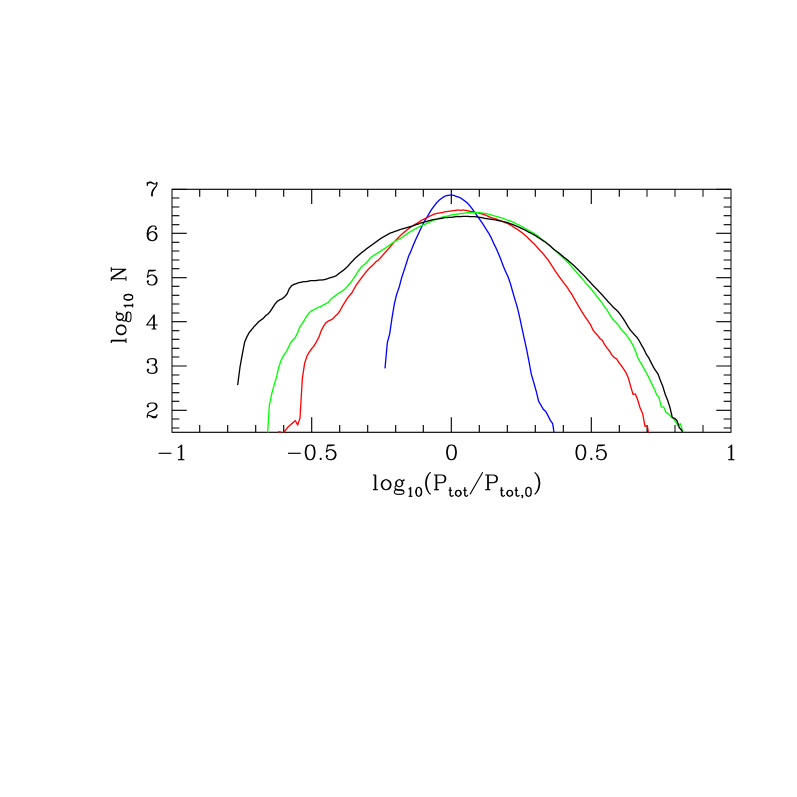
Figure 3: Frequency distribution of the total (gas and magnetic) pressure. The blue, red, green, and black lines are for the simulations with $\beta_{0}$ = 0.1, 1, 10, and 100, respectively.

Beck et al. (2003) pointed that the discrepancy in the strengths of the regular Galactic magnetic field estimated with RM and synchrotron emissivity could be reconciled, if the correlation between $B$ and $n_{e}$ is negative in the WIM and so the RM field was underestimated. Beck et al. (2003) postulated the pressure equilibrium, which results in the negative correlation between $B$ and $\rho$. If the pressure equilibrium is maintained, the combined pressure of gas and magnetic field, $P_{\rm tot}=P_{\rm gas}+P_{\rm mag}$, should exhibit a narrow distribution. Figure 3 shows the frequency distribution of $P_{\rm tot}$. Our simulations show broad distributions rather than peaked distributions. That is, our results do not support the prediction of Beck et al. (2003). However, we caution that we considered only the turbulent media with the rms Mach number $M_{s}=1$. On the other hand, the WIM may have $M_{s}$ which is not exactly unity. So we need to further investigate turbulent media with $M_{s}\neq 1$, before we exclude the postulation of Beck et al. (2003). We leave it as a future work.

4 Frequency Distribution of RMs

We then look at the frequency distribution of RMs. Figure 4 shows the probability distribution of RM/$\overline{\rm RM}$ for different $\beta_{0}$’s as well as for different $\theta$’s. Here, $\overline{\rm RM}$ is the average value of RMs. (The distribution was also calculated for $\theta=83^{\circ}$, but not shown in the figure for clarity. The distribution for $\theta=83^{\circ}$ is used in Figure 5.) The fit to the Gaussian is also shown. A noticeable point in the figure is that the distribution of RM/$\overline{\rm RM}$ is very well fitted to the Gaussian. The goodness-of-fit is between 0.89 and 0.99 . This result is consistent with the observations of Haverkorn et al. (2003, 2004). They took the multi-frequency polarimetric images of diffuse radio synchrotron backgrounds in the constellation Auriga and Horologium, and obtained RM maps. The distribution of the observed RMs is also fitted to the Gaussian.

Another noticeable point in Figure 4 is that the distribution is more widely spread for larger $\beta_{0}$ and larger $\theta$. It hints at a possible correlation between the spread in the distribution of RM/$\overline{\rm RM}$ with the strength of the magnetic field along the line of sight. Figure 5 shows the relation between the full width at half maximum, $W_{\rm FWHM}$, of the distribution of RM/$\overline{\rm RM}$ shown in Figure 4 and the strength of the regular field along the line of sight, $B_{0\parallel}\equiv\ B_{0}\cos\theta$. The best fit for the relation is

$$B_{0\parallel}=(2.45\pm 0.3)\times W_{\rm FWHM}^{-1.41\pm 0.1}~{}~{}\mu{\rm G}.$$ (3)

Note that the relation is for $T=8000$ K and $n_{e}=0.03$ cm^-3 as the representative values of the temperature and electron density, and scales as $(T/8000~{}{\rm K})^{1/2}(n_{e}/0.03~{}{\rm cm}^{-3})^{1/2}$ for other values of $T$ and $n_{e}$. The empirical relation in (3) may provide a handy way to quantify the strength of the regular field along the line of sight in regions where the map of RMs has been obtained along many contiguous lines of sight with the multi-frequency polarimetric observations (see Introduction). The accompanying map of DMs is not necessary for it.

The estimation of magnetic field strength with the relation in (3), however, should be done with caution because of its limitations: First, the relation is valid only for $M_{s}=1$. Second, no stratification of gas and magnetic field was assumed, which is apparent in the polarization maps of a larger area of our Galaxy. Third, no source emitting polarized light in the medium between background polarized continua and us was considered.

From a physical point of view, the broadening of the width of RM distribution is due to fluctuating magnetized gas. We can easily expect that, for a given regular field, the width would be larger if the rms Mach number, $M_{s}$, is larger. So $W_{\rm FWHM}$ should be a function of not only $B_{0\parallel}$ but also $M_{s}$. In order to quantify the relation of $W_{\rm FWHM}$ versus $B_{0\parallel}$ and $M_{s}$, we need simulations that cover the parameter space of $\beta_{0}$ and $M_{s}$. Low-resolution simulations with $M_{s}=0.5$ and 2.0 show that the probability distribution of RM/$\overline{\rm RM}$ is still fitted to the Gaussian, and $W_{\rm FWHM}$ can differ by a factor of two to three if $M_{s}$ differs by a factor of two. We leave the report of the $M_{s}\neq 1$ results, including the correlation between $B$ and $\rho$, from high-resolution simulations as a future work.

Nevertheless, we can try to apply the relation in (3) to RM observations in the WIM, assuming $M_{s}=1$ there. For instance, from the figures of the frequency distribution of RMs in Auriga and Horologium in Haverkorn et al. (2003, 2004), we read $W_{\rm FWHM}\simeq 2$ and 7, and get $B_{0\parallel}\sim 0.6$ and 0.1 $\mu$G for Auriga and Horologium, respectively (if $n_{e}=0.016$ cm^-3 is used as in Haverkorn et al. (2004)). These are close to, but somewhat larger than, the values estimated in Haverkorn et al. (2004), $\sim 0.42$ and 0.085 $\mu$G, respectively. However, by considering the limitations of the relation in (3) and the uncertainty in the values of $W_{\rm FWHM}$ which we read from figures, we regard the agreement to be fair.

Currently the number of the synchrotron backgrounds, which can be used for the observation of RM maps, is still limited due to the relatively low sensitivity of present-day radio telescopes. However, the new-generation radio telescopes, such as LOFAR (Low Frequency Array) and SKA (Square Kilometer Array) with much higher sensitivity, will certainly provide RM maps in much larger portions of the sky. Then, the relation like the one in (3) will become a useful diagnosis.

Figure 1: Contour plots showing the correlation between the magnetic field strength and the gas density at the end of fours simulations. The contour levels are from 10% to 90% of the peak value with the interval of 10%.

Figure 2: Frequency distribution of (a) $\langle B_{x}\rangle$ and (b) $\langle B_{y}\rangle$, normalized with the initial magnetic field strength, $B_{0}$. The solid lines present the true mean strength of the magnetic field along the line of sight, and the dotted lines present the magnetic field strength calculated with RM/DM, along $512^{2}$ lines aligned the (a) $x$ and (b) $y$-axes. The blue, red, green, and black lines are for the simulations with $\beta_{0}$ = 0.1, 1, 10, and 100, respectively.

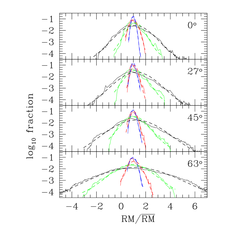
Figure 4: Probability distribution of RMs normalized with the average value. The solid lines are the distribution, and the corresponding dashed lines are the Gaussian fit. The blue, red, green, and black lines are for $\beta_{0}$ = 0.1, 1, 10, and 100, respectively. Different panels are for different values of $\theta$ (the angle between the direction of the regular field and the line of sight).

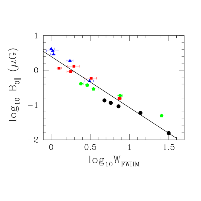
Figure 5: Relation between the full width at half maximum of the distribution of RM/$\overline{\rm RM}$ ($W_{\rm FWHM}$) and the strength of the regular field along the line of sight ($B_{0\parallel}$). Blue, red, green, and black symbols are from the simulations with $\beta_{0}$ = 0.1, 1, 10, and 100, respectively (for five different $\theta$’s including $\theta=83^{\circ}$). The error bar shows the error in the Gaussian fit in Figure 4. The solid line shows the best fit of the relation between $W_{\rm FWHM}$ and $B_{0\parallel}$.

References

- Armstrong et al. (1995) Armstrong, J. W., Rickett, B. J., & Spangler, S. R. 1995, ApJ, 443, 209
- Balsara & Kim (2005) Balsara, D. S., & Kim, J. 2005, ApJ, 634, 390
- Beck (2007) Beck, R. 2007, A&A, 470, 539
- Beck et al. (2003) Beck, R., Shukurov, A, Sokoloff, D., & Wielebinski, R. 2003, A&A, 411, 99
- Berkhuijsen & Fletcher (2008) Berkhuijsen, E. M., & Fletcher, A. 2008, MNRAS, 390, L19
- Burkhart et al. (2009) Burkhart, B., Falceta-Goncalves, D., Kowal, G., & Lazarian, A. 2009, ApJ, 693, 250
- Crutcher (1999) Crutcher, R. M. 1999, ApJ, 520, 706
- de Bruyn & Brentjens (2005) de Bruyn, A. G., & Brentjens, M. A. 2005, A&A, 441, 931
- Elmegreen & Scalo (2004) Elmegreen, B. G., & Scalo, J. 2004, ARA&A, 42, 211
- Frick et al. (2001) Frick, P., Stepanov, R., Shukurov, A., & Sokoloff, D. 2001, MNRAS, 325, 649
- Haffner et al. (1999) Haffner, L. M., Reynolds, R. J., & Tufte, S. L. 1999, ApJ, 523, 223
- Han et al. (1998) Han, J. L., Beck, R., & Berkhuijsen, E. M. 1998, A&A, 335, 1117
- Han et al. (2006) Han, J. L., Manchester, R. N., Lyne, A. G., Qiao, G. J., & van Straten, W. 2006, ApJ, 642, 868
- Han & Wielebinski (2002) Han, J. L., & Wielebinski, R. 2002, Chinese J. Astron. Astrophys., 2, 293
- Haverkorn et al. (2003) Haverkorn, M., Katgert, P., & de Bruyn, A. G. 2003, A&A, 403, 1031
- Haverkorn et al. (2004) Haverkorn, M., Katgert, P., & de Bruyn, A. G. 2004, A&A, 427, 167
- Heiles & Troland (2003) Heiles, C., & Troland, T. H. 2003, ApJ, 586, 1067
- Hill et al. (2008) Hill, A. S., Benjamin, R. A., Kowal, G., Reynolds, R. J., Haffner, M., & Lazarian, A. 2008, ApJ, 686, 363
- Indrani & Deshpande (1999) Indrani, C., & Deshpande, A. A. 1999, New A, 4, 33
- Kim et al. (1999) Kim, J., Ryu, D., Jones, T. W., & Hong, S. S. 1999, ApJ, 514, 506
- Larson (1981) Larson, R. B. 1981, MNRAS, 194, 809
- Mac Low (1999) Mac Low, M.-M. 1999, ApJ, 524, 169
- Mac Low et al. (2005) Mac Low, M.-M., Balsara, D. S., Kim, J., & de Avillez, M. A. 2005, ApJ, 626, 864
- Ostriker et al. (2001) Ostriker, E. C., Stone, J. M., & Gammie, C. F. 2001, ApJ, 546, 980
- Padoan & Nordlund (1999) Padoan, P., & Nordlund, A. 1999, ApJ, 526, 279
- Passot & Vázquez-Semadeni (2003) Passot, T., & Vázquez-Semadeni, E. 2003, A&A, 398, 845
- Reynolds (1985) Reynolds, R. J. 1985, ApJ, 294, 256
- Reynolds (1991) Reynolds, R. J. 1991, ApJ, 372, L17
- Schnitzeler et al. (2009) Schnitzeler, D. H. F. M., Katgert, P., & de Bruyn, A. G. 2009, A&A, 494, 611
- Spitzer (1978) Spitzer, L. 1978, Physical Processes in the Interstellar Medium (New York: Wiley)
- Stone et al. (1999) Stone, J. M., Ostriker, E. C., & Gammie, C. F. 1998, ApJ, 508, L99
- Tufte et al. (1999) Tufte, S. L., Reynolds, R. J., & Haffner, L. M. 1999, in Interstellar Turbulence, ed. J. Franco & A. Carraminana (Cambridge: Cambridge Univ. Press), p27
- Vázquez-Semadeni (1994) Vázquez-Semadeni, E. 1994, ApJ, 423, 681