Update on onium masses with three flavors of dynamical quarks

Abstract:

We update results presented at Lattice 2005 on charmonium masses. New ensembles of gauge configurations with 2+1 flavors of improved staggered quarks have been analyzed. Statistics have been increased for other ensembles. New results are also available for $P$-wave mesons and for bottomonium on selected ensembles.

1 Introduction

The calculation of the onium spectrum from first principles from lattice QCD represents a significant goal. There are a number of states that are stable to strong decay and far from thresholds (that might make finite size effects more significant). It should be possible to accurately calculate all of their masses. Further, since there are no valence up and down quarks, we have to consider only the sea quark mass dependence. However, one must be careful in dealing with heavy quarks on the lattice because $aM$ is not small. Some early results using dynamical quark configurations were published in 2004 [1]. Using clover type quarks with the Fermilab interpretation [2], we have been calculating the onium spectrum for some time [3] on MILC gauge configurations [4]. The HPQCD/UKQCD collaborations have successfully been using NRQCD to treat the bottom quark on many of the same ensembles [5]. Recently, they have started to use highly improved staggered quarks (HISQ) to study charm [6].

At Lattice 2005 [7], we presented results for lattice spacings $a\approx 0.18$, 0.12 and 0.09 fm. These are denoted extra coarse, coarse and fine, respectively. This year we have several new ensembles with a lattice spacing of $\approx 0.15$ fm, denoted medium coarse in the plots. On these new ensembles, we have tuned the dynamical strange quark mass closer to its physical value based upon experience with the earlier ensembles. At the fine lattice spacing, we have new results on a more chiral ensemble with $am_{l}=0.0031$ and $am_{s}=0.031$ on a $40^{3}\times 96$ grid. All of our results for bottomonium are new. We also have some new results for the $\chi_{c2}$. (See Table 1 for details of the ensembles.)

$am_{q}$ / $am_{s}$	$10/g^{2}$	$\approx a$	size	volume	config.
0.0492 / 0.082	6.503	0.18	$16^{3}\times 48$	$(2.8\;{\rm fm})^{3}$	401
0.0328 / 0.082	6.485	0.18	$16^{3}\times 48$	$(2.8\;{\rm fm})^{3}$	331
0.0164 / 0.082	6.467	0.18	$16^{3}\times 48$	$(2.8\;{\rm fm})^{3}$	645
0.0082 / 0.082	6.458	0.18	$16^{3}\times 48$	$(2.8\;{\rm fm})^{3}$	400
0.0194 / 0.0484	6.586	0.15	$16^{3}\times 48$	$(2.4\;{\rm fm})^{3}$	631
0.0097 / 0.0484	6.566	0.15	$20^{3}\times 48$	$(3.0\;{\rm fm})^{3}$	631
0.03 / 0.05	6.81	0.12	$20^{3}\times 64$	$(2.4\;{\rm fm})^{3}$	549
0.02 / 0.05	6.79	0.12	$20^{3}\times 64$	$(2.4\;{\rm fm})^{3}$	460
0.01 / 0.05	6.76	0.12	$20^{3}\times 64$	$(2.4\;{\rm fm})^{3}$	593
0.007 / 0.05	6.76	0.12	$20^{3}\times 64$	$(2.4\;{\rm fm})^{3}$	403
0.005 / 0.05	6.76	0.12	$24^{3}\times 64$	$(2.9\;{\rm fm})^{3}$	397
0.0124 / 0.031	7.11	0.09	$28^{3}\times 96$	$(2.4\;{\rm fm})^{3}$	517
0.0062 / 0.031	7.09	0.09	$28^{3}\times 96$	$(2.4\;{\rm fm})^{3}$	557
0.0031 / 0.031	7.08	0.09	$40^{3}\times 96$	$(3.4\;{\rm fm})^{3}$	504

Table 1: Ensembles used in this calculation.

To calculate the onium spectrum, we need to find an appropriate value of the heavy quark hopping parameter $\kappa$. We do this by studying the $D_{s}$ and $B_{s}$ kinetic masses. We do this study on one ensemble for each lattice spacing and use the selected values of $\kappa_{c}$ and $\kappa_{b}$ for all the ensembles with that lattice spacing. Errors in the kinetic masses tend to be large, and so we calculate mass splittings based on differences in the rest energy.

2 Charmonium Results

We will examine a number of splittings in the charmonium spectrum. Let’s look at the difference between the spin averaged $2S$ and $1S$ states. In Fig. 2, we plot the splitting in MeV as a function of the light bare sea quark mass. The experimental value is shown as a black fancy cross. The points in red are linear extrapolations in quark mass. We find that at each lattice spacing (except for the fine lattice) the extrapolated value is in good agreement with experiment. On the fine lattice, there is a considerable slope and the extrapolated value is quite high. (We note that as the horizonal axis is the bare quark mass, the slope is not a physical quantity; it also reflects a change in the mass renormalization as the lattice spacing changes.)

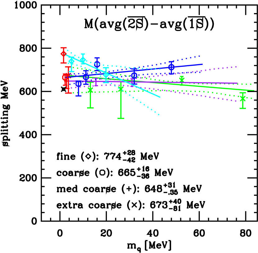
Figure 1: Splitting between the spin-averaged $2S$ and $1S$ states of charmonium.

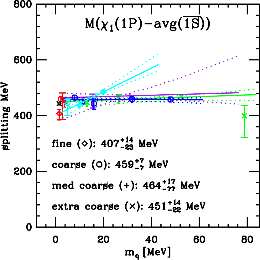
Figure 2: Splitting between the $\chi_{c1}(1P)$ and spin-averaged $1S$ states.

Next we turn to issues of fine structure and look at the splitting between the $\chi_{c1}(1P)$ and the spin averaged $1S$ mass. It would be more natural to compare with the spin average of all the $1P$ states, but the $\chi_{c2}$ mass is not yet available on all ensembles, so we compare with the $1S$ spin average. Using the same color scheme and symbols as in the previous figure, we see in Fig. 2, that there is good agreement with experiment except on the fine ensembles which again exhibit a substantial slope. In this case, the two more chiral ensembles are in good agreement with the experimental value, but the ensemble with the heaviest value of the light sea quark mass gives too large a value for the splitting, leading to a large slope and too small a chiral limit.

For the $h_{c}(1P)$ state shown in Fig. 4, we find good agreement with the experimental value on all ensembles. For the finest lattice spacing, there is only a modest slope from the chiral extrapolation.

Turning next to the hyperfine splitting, we look at the $J/\psi(1S)$ – $\eta_{c}(1S)$ mass splitting in Fig. 4. In this case, we find that the splittings are sytematically small, but that the value is increasing toward the experimental value as the lattice spacing decreases.

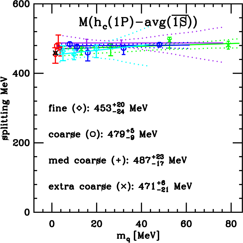
Figure 3: Splitting between the $h_{c}(1P)$ and spin-averaged $1S$ states.

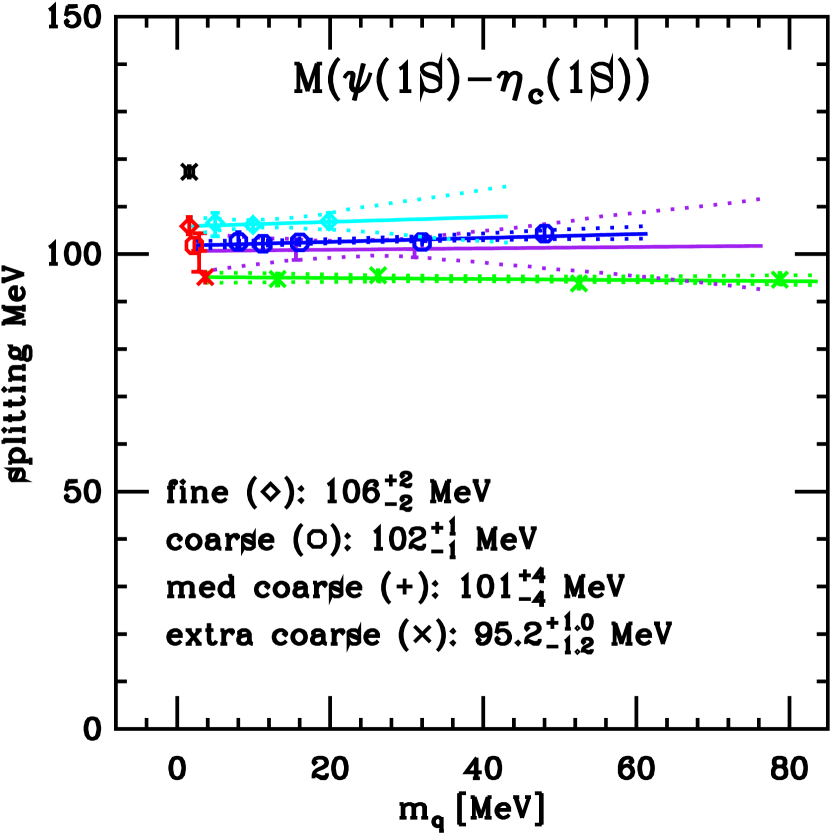
Figure 4: Hyperfine splitting of the $1S$ states.

The $\chi_{c2}(1P)$ has only been studied on two ensembles so far. We have new results on one fine ensemble. In Fig. 5, we summarize the results for all the states studied. Except for the $\chi_{c2}(1P)$, we plot results from our linear chiral extrapolation for each lattice spacing. For the ground states, if we focus our attention on the diamonds representing our smallest lattice spacing, we find the most serious discrepancy between our results and experiment is for the $\chi_{c1}$. We have seen that our linear chiral extrapolation may be the culprit here, as the two more chiral ensembles are in good agreement with the experimental value. The $S$ wave first excited states are not that well determined, but are rather heavy compared to the observed values. We have seen that on the finest lattice spacing, the high slope of the chiral extrapolation is accentuating the difference between our calculation and observations. Furthermore, the observed states are quite close to the $D\bar{D}$ threshold, which makes these states harder to calculate on the lattice without careful attention to finite volume effects. Thus, we are not seriously concerned about the high masses we are seeing for the 2$S$ states.

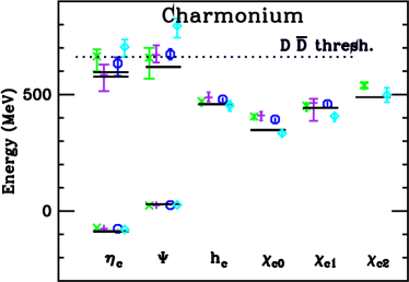
Figure 5: Summary of charmonium spectrum.

3 Bottomonium Results

We have new results this year for bottomonium on the three smallest lattice spacings. Some important ground states in this system, the $\eta_{b}$ and $h_{b}$, have not been observed, so we shall modify some of the splittings we display. It is also interesting to compare our results with those using NRQCD for the heavy quarks [5]. We expect that our results have larger discretization errors, when comparing them to the results of Ref. [5] at a fixed lattice spacing, because the NRQCD action used in that work is more improved.

In Fig. 7, we plot the splitting between the $\Upsilon(2S)$ and $\Upsilon(1S)$ masses. On the fine ensembles, the result is in good agreement with experiment. With larger lattice spacings, the splitting is a bit low. We look only at the $\Upsilon$ level since the $\eta_{b}$ masses are not well measured. In the bottomonium system, the $2S$ and $3S$ states are both below the $B\bar{B}$ threshold. Thus, possible finite size effects from a nearby threshold are not an issue, and we should get the $2S$ levels right.

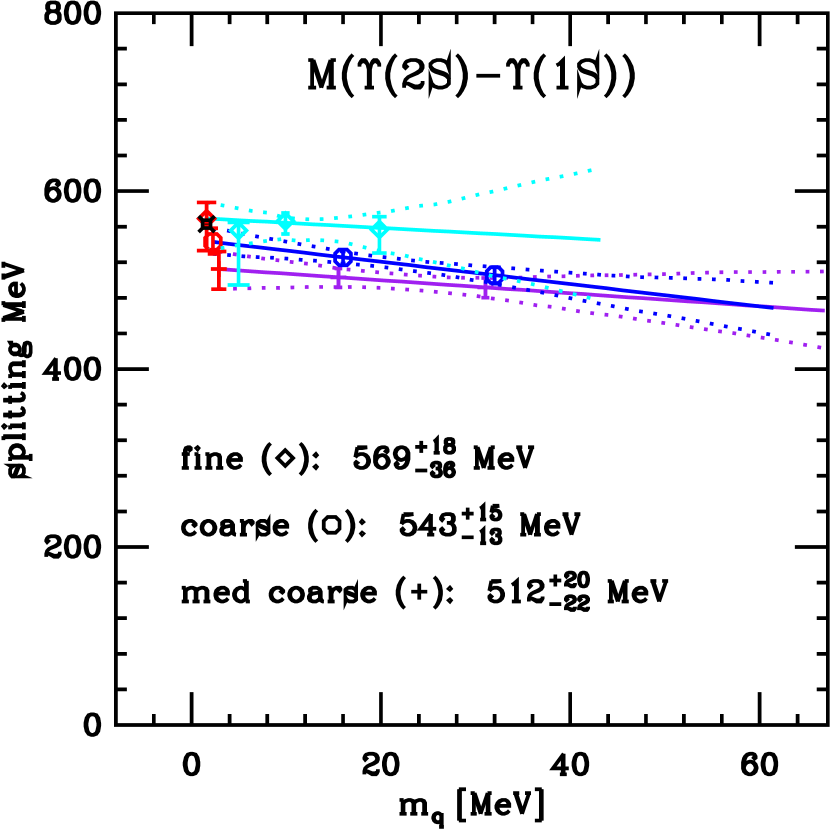
Figure 6: Chiral extrapolation of the $\Upsilon(2S)$-$\Upsilon(1S)$ splitting.

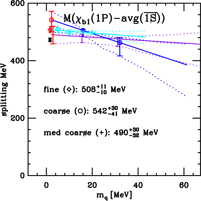
Figure 7: Chiral extrapolation of the $\chi_{b1}(1P)$ – spin averaged $1S$ splitting.

In considering the fine structure of the bottomonium spectrum we are faced with two issues. First, the $h_{b}$ has not been observed so we cannot compare our results with the experimental value (but we can make a prediction). Second, we have no results for $\chi_{b2}$ yet, so we can’t compute a spin average of the $P$ states. So, we consider the $\chi_{b1}$, in the middle of the three ${}^{3}P_{J}$ states. We compare it to the spin averaged $1S$ states assuming our $\eta_{b}$ mass is correct. The result shown in Fig. 7 has the splitting about 35 MeV too large on the fine lattices.

The hyperfine splitting in the $1S$ states is shown in Fig. 9. We find a value of about 38 MeV for this splitting for all $a$. The experimental result plotted comes from the PDG and is based on the observation of a single $\eta_{b}$. It should be noted that a preliminary result from CDF with higher statistics had a splitting of only 15 MeV. With this factor of 10 difference between the experimental results, it is hard to reach any definite conclusion about how accurate our hyperfine splitting is for the $1S$ states. It turns out, however, that on four ensembles we can directly compare our calculation with the HPQCD results. In Fig. 9, we compare the splitting in lattice units. The results are plotted on a semilogarithmic scale so that equal vertical differences represent equal fractional differences in the splittings. The upper two octagons and diamonds are coarse lattice results. The lower two octagons and diamonds are on fine ensembles. Points with the same bare quark mass are calculated on the same ensembles, but the HPQCD collaboration did not analyze every available configuration, so the actual set of configurations selected for analysis differs. We see that the fraction difference in the hyperfine splittings is larger at the smaller lattice spacing and that the NRQCD hyperfine splitting is larger than that for clover. The difference is not unexpected, because the leading error for this splitting with the clover action is of order $mv^{6}$, whereas in Ref. [5] it is of order $mv^{8}$.

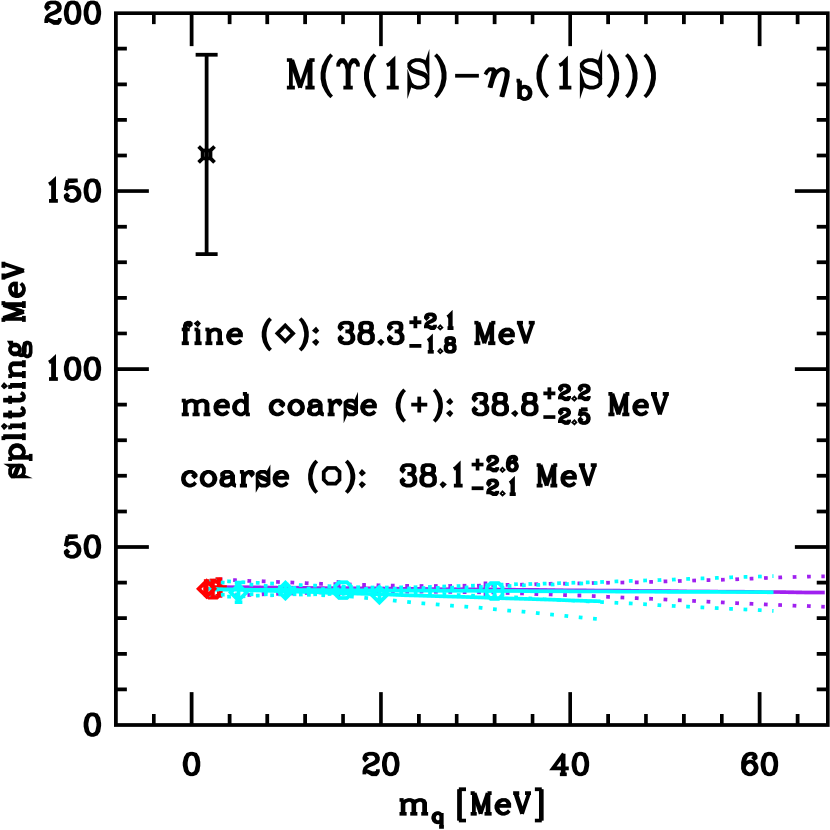
Figure 8: Hyperfine splitting of the bottomonium $1S$ states.

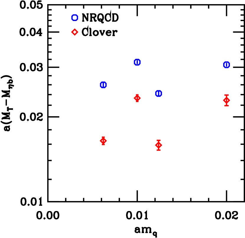
Figure 9: Comparison of HPQCD’s hyperfine splitting using NRQCD with this work.

In Fig. 10, we summarize the spectrum of observed states using the spin-averged $1S$ states (assuming a 38 MeV $\Upsilon$–$\eta_{b}$ splitting) to set the additive constant needed to go from splittings to masses. Solid lines on the plot are experimentally determined masses. Dashed lines on the plot denote unobserved (or poorly observed) states. In the case of the $\eta_{b}$ we use dashed lines and mark them CDF and PDG as discussed above. We find good agreement with experiment for the $\Upsilon(2S)$. The $\eta_{b}(2S)$ is in good agreement with theoretical expectations. Our masses for the $P$ wave states $h_{b}$, $\chi_{b0}$ and $\chi_{b1}$ are too large.

Figure 10: Summary of the bottomonium spectrum for ensembles with $a\approx 0.15$, 0.12 and 0.09 fm.

4 Conclusions and Outlook

We observe only a mild dependence on the sea quark mass for most of the quantities studied here. In particular, the hyperfine splittings and the $2S$-$1S$ splittings appear to be essentially independent of the sea quark mass. Hence a linear extrapolation seems adequate. For the $P$-wave states, we do observe a sea quark mass dependence at the 10% level on some ensembles.

There are several positive features of the charmonium spectrum. The $h_{c}$ and $\chi_{c1}$ masses look quite good (although the latter is driven low by the chiral extrapolation on the fine ensembles). At the smallest lattice spacing studied so far, the $P$ wave splitting looks good (but see previous sentence). The hyperfine splitting is too small but improving as the lattice spacing decreases. However, the $2S$ states are not accurately calculated. For the bottomonium spectrum, the excited state splitting looks good. It is not yet possible to test the hyperfine splitting, but our splitting is smaller than that coming from NRQCD calculations. Our $P$ wave states seem too heavy.

In the coming year, we expect to increase our statistics on a number of existing ensembles. In addition, MILC is generating ensembles with a lattice spacing of 0.06 fm and has plans to reduce the lattice spacing to 0.045. There is also some chance that there will be some ensembles with $a=0.105$ fm. Currently, we are using an automatic criterion for picking the best fit. We need to consider alternative methods and whether picking a single fit properly reflects the systematic errors.

The $P$ wave splitting in the bottomonium spectrum does not seem to be in agreement with experiment. It will be interesting to see if the bottomonium spectrum improves as we reduce the lattice spacing (and $am_{b}$). Kronfeld and Oktay [8] have been developing a highly improved clover quark action that we hope to use in the future.

References

- [1] C. Davies et al. [Fermilab Lattice, HPQCD, MILC, UKQCD], Phys. Rev. Lett. 92 (2004) 022001 [hep-lat/0304004].
- [2] A. El-Khadra, A.S. Kronfeld, P.B. Mackenzie, Phys. Rev. D 55 (1997) 3933 [hep-lat/9604004].
- [3] M. di Pierro et al., Nucl. Phys. B (Proc. Suppl.) 129 (2004) 340 [hep-lat/0310042].
- [4] C. Bernard et al. [MILC], Phys. Rev. D 64 (2001) 054506 [hep-lat/0104002]; C. Aubin et al. [MILC], Phys. Rev. D 70 (2004) 094505 [hep-lat/0402030].
- [5] A. Gray et al.[HPQCD, UKQCD], Phys. Rev. D 72 (2005) 094507 [hep-lat/0507013].
- [6] E. Follana et al.[HPQCD] [hep-lat/0610092]; Nucl. Phys. B (Proc. Suppl.) 129 (2004) 447 [hep-lat/0311004]; 129 (2004) 384 [hep-lat/0406021].
- [7] S. Gottlieb et al., \posPoS(LAT2005)203 [hep-lat/0510072].
- [8] A.S. Kronfeld and M.B. Oktay, \posPoS(LAT2006)159 [hep-lat/0610069]; M.B. Oktay et al., Nucl. Phys. B (Proc. Suppl.) 129 (2004) 349 [hep-lat/0309107]; 119 (2003) 464 [hep-lat/0209150].