A Tasty Combination:
Multivariable Calculus and Differential Forms

Abstract.

Differential Calculus is a staple of the college mathematics major’s diet. Eventually one becomes tired of the same routine, and wishes for a more diverse meal. The college math major may seek to generalize applications of the derivative that involve functions of more than one variable, and thus enjoy a course on Multivariate Calculus. We serve this article as a culinary guide to differentiating and integrating functions of more than one variable – using differential forms which are the basis for de Rham Cohomology.

Introduction

Differential Calculus is a staple of the college mathematics major’s diet. It is relatively easy to explain the Fundamental Theorem of Calculus: Given a differentiable function $f:I\to\mathbb{R}$ defined on closed interval $I=[a,b]$, there is the identity

$$\int_{a}^{b}\frac{d}{dt}\bigl{[}f(t)\bigr{]}dt=f(b)-f(a).$$

Eventually one becomes tired of the same routine, and wishes for a more diverse meal. The college math major may seek to generalize applications of the derivative that involve functions of more than one variable, and thus enjoy a course on Multivariate Calculus. Actually, there is a veritable buffet of ways to differentiate and integrate a function of more than one variable: there is the gradient, curl, divergence, path integrals, surface integrals, and volume integrals. Plus, there are many “Fundamental” Theorems of Multivariate Calculus, such as Stokes’ Theorem, Green’s Theorem, and Gauss’ Theorem.

We serve this article as a culinary guide to differentiating and integrating functions of more than one variable – using differential forms which are the basis for de Rham Cohomology.

Gradient, Curl, and Divergence

Let’s focus on functions of three variables. First, let’s fix a “simply connected” closed subset $D\subseteq\mathbb{R}^{3}$; this means we can define an integral between two points without concern of a choice of path in $D$ which connects them. (For example, a subset in the form $D=[a,b]\times[c,d]\times[p,q]$ is simply connected.) Recall that the gradient of a scalar function $f:D\to\mathbb{R}$ is the vector-valued function $\nabla f:D\to\mathbb{R}^{3}$ defined by

$$\nabla f=\frac{\partial f}{\partial x}\,\mathbf{i}+\frac{\partial f}{\partial y}\,\mathbf{j}+\frac{\partial f}{\partial z}\,\mathbf{k}.$$

(Here $\mathbf{i}=(1,0,0)$, $\mathbf{j}=(0,1,0)$, and $\mathbf{k}=(0,0,1)$ are the standard basis vectors for 3-dimensional space.) The curl of a vector field $\mathbf{F}:D\to\mathbb{R}^{3}$, which we write in the form $\mathbf{F}=M\,\mathbf{i}+N\,\mathbf{j}+P\,\mathbf{k}$, is the vector-valued function $\nabla\times\mathbf{F}:D\to\mathbb{R}^{3}$ defined by

$$\nabla\times\mathbf{F}=\left|\begin{matrix}\mathbf{i}&\mathbf{j}&\mathbf{k}\\[8.0pt] \dfrac{\partial}{\partial x}&\dfrac{\partial}{\partial y}&\dfrac{\partial}{\partial z}\\[8.0pt] M&N&P\end{matrix}\right|=\left(\frac{\partial P}{\partial y}-\frac{\partial N}{\partial z}\right)\mathbf{i}+\left(\frac{\partial M}{\partial z}-\frac{\partial P}{\partial x}\right)\mathbf{j}+\left(\frac{\partial N}{\partial x}-\frac{\partial M}{\partial y}\right)\mathbf{k}.$$

(If you don’t remember how to compute $3\times 3$ determinants, don’t worry; we have a short exposition on them contained in the appendix.) Finally, the divergence of a vector field $\mathbf{G}:D\to\mathbb{R}^{3}$, which we write in the form $\mathbf{G}=S\,\mathbf{i}+T\,\mathbf{j}+U\,\mathbf{k}$, is the scalar function $\nabla\cdot\mathbf{G}:D\to\mathbb{R}$ defined by

$$\nabla\cdot\mathbf{G}=\frac{\partial S}{\partial x}+\frac{\partial T}{\partial y}+\frac{\partial U}{\partial z}.$$

Larson [4] provides more information on Multivariable Calculus. Marsden and Tromba [5] is also an excellent source. Hughes-Hallet et al. [3] provides a novel approach to the subject using concept-based learning.

We would like to answer the following questions:

1. Which $\mathbf{F}:D\to\mathbb{R}^{3}$ have a scalar potential $f:D\to\mathbb{R}$ such that $\mathbf{F}=\nabla f$?

2. Which $\mathbf{G}:D\to\mathbb{R}^{3}$ have a vector potential $\mathbf{F}:D\to\mathbb{R}^{3}$ such that $\mathbf{G}=\nabla\times\mathbf{F}$?

3. Which $f:D\to\mathbb{R}$ have a vector potential $\mathbf{G}:D\to\mathbb{R}^{3}$ such that $f=\nabla\cdot\mathbf{G}$?

Relating Gradients and Curls

Let’s answer the first of our motivating questions. We’ll show the following:

$\mathbf{F}=\nabla f$ is a gradient if and only if the curl $\nabla\times\mathbf{F}=\mathbf{0}$.

First assume that $\mathbf{F}=\nabla f$. That is, $\mathbf{F}=M\,\mathbf{i}+N\,\mathbf{j}+P\,\mathbf{k}=\dfrac{\partial f}{\partial x}\,\mathbf{i}+\dfrac{\partial f}{\partial y}\,\mathbf{j}+\dfrac{\partial f}{\partial z}\,\mathbf{k}.$ To find the curl of $\mathbf{F}$, we have

$$\nabla\times\mathbf{F} =\left(\frac{\partial P}{\partial y}-\frac{\partial N}{\partial z}\right)\mathbf{i}+\left(\frac{\partial M}{\partial z}-\frac{\partial P}{\partial x}\right)\mathbf{j}+\left(\frac{\partial N}{\partial x}-\frac{\partial M}{\partial y}\right)\mathbf{k}$$

$$=\left(\frac{\partial^{2}f}{\partial y\,\partial z}-\frac{\partial^{2}f}{\partial z\,\partial y}\right)\mathbf{i}+\left(\frac{\partial^{2}f}{\partial z\,\partial x}-\frac{\partial^{2}f}{\partial x\,\partial z}\right)\mathbf{j}+\left(\frac{\partial^{2}f}{\partial x\,\partial y}-\frac{\partial^{2}f}{\partial y\,\partial x}\right)\mathbf{k}$$

$$=\mathbf{0}.$$

Note that we can change the order of differentiation as long as $f$ is continuously twice-differentiable: with this assumption, Clairaut’s Theorem states that the mixed partial derivatives are equal. (This theorem and its proof can be found in [6, pgs. 885 and A-48].)

Now what if $\nabla\times\mathbf{F}=\mathbf{0}$? Can we find an $f$ such that $\mathbf{F}=\nabla f$? Well, if $\nabla\times\mathbf{F}=\mathbf{0}$, then

$$\left(\frac{\partial P}{\partial y}-\frac{\partial N}{\partial z}\right)=\left(\frac{\partial M}{\partial z}-\frac{\partial P}{\partial x}\right)=\left(\frac{\partial N}{\partial x}-\frac{\partial M}{\partial y}\right)=0.$$

Now define the scalar function $f=u+v+w$ in terms of the definite integrals

$$u(x,y,z) =\int_{x_{0}}^{x}M(\sigma,\,y,\,z)\,d\sigma,$$

$$v(x,y,z) =\int_{y_{0}}^{y}\left[N(x,\tau,z)-\frac{\partial u}{\partial y}(x,\tau,z)\right]d\tau,$$

$$w(x,y,z) =\int_{z_{0}}^{z}\left[P(x,y,\zeta)-\frac{\partial u}{\partial z}(x,y,\zeta)-\frac{\partial v}{\partial z}(x,y,\zeta)\right]d\zeta$$

where we have fixed a point $x_{0}\,\mathbf{i}+y_{0}\,\mathbf{j}+z_{0}\,\mathbf{k}\in D$. (Here’s where we subtly use the assumption that $D$ is simply connected: the integrals are independent of a choice of path in $D$ which connects $x_{0}\,\mathbf{i}+y_{0}\,\mathbf{j}+z_{0}\,\mathbf{k}$ and $x\,\mathbf{i}+y\,\mathbf{j}+z\,\mathbf{k}$.) Upon changing the order of differentiation and integration, we have the derivatives

$$\frac{\partial v}{\partial x} =\int_{y_{0}}^{y}\left[\frac{\partial N}{\partial x}-\frac{\partial M}{\partial y}\right]d\tau=0,$$

$$\frac{\partial w}{\partial x} =\int_{z_{0}}^{z}\left[\left(\frac{\partial P}{\partial x}-\frac{\partial M}{\partial z}\right)-\frac{\partial v}{\partial x}\right]d\zeta=0,$$

$$\frac{\partial w}{\partial y} =\int_{z_{0}}^{z}\left[\frac{\partial P}{\partial y}-\frac{\partial}{\partial z}\left(\frac{\partial u}{\partial y}+\frac{\partial v}{\partial y}\right)\right]d\zeta=\int_{z_{0}}^{z}\left[\frac{\partial P}{\partial y}-\frac{\partial N}{\partial z}\right]d\zeta=0.$$

(We can only do this if $M$, $N$, and $P$ are continuously differentiable functions; this also follows from Clairaut’s Theorem.) It follows that $\mathbf{F}=\nabla f$:

$$\nabla f=\biggl{[}\frac{\partial u}{\partial x}+\cancelto{0}{\frac{\partial v}{\partial x}}+\cancelto{0}{\frac{\partial w}{\partial x}}\biggr{]}\mathbf{i}+\biggl{[}\frac{\partial u}{\partial y}+\frac{\partial v}{\partial y}+\cancelto{0}{\frac{\partial w}{\partial y}}\biggr{]}\mathbf{j}+\biggl{[}\frac{\partial u}{\partial z}+\frac{\partial v}{\partial z}+\frac{\partial w}{\partial z}\biggr{]}\mathbf{k}=M\,\mathbf{i}+N\,\mathbf{j}+P\,\mathbf{k}.$$

We conclude that $\mathbf{F}:D\to\mathbb{R}^{3}$ has a scalar potential $f:D\to\mathbb{R}$ such that $\mathbf{F}=\nabla f$ if and only if the curl $\nabla\times\mathbf{F}=\mathbf{0}$.

Example

Let’s see this result in action. Consider the scalar function

$$f(x,y,z)=\sqrt{x^{2}+y^{2}+z^{2}}.$$

We compute the gradient using the Chain Rule:

$$\frac{\partial f}{\partial x} =\frac{1}{2}\left(x^{2}+y^{2}+z^{2}\right)^{-1/2}\cdot 2\,x=\frac{x}{\sqrt{x^{2}+y^{2}+z^{2}}},$$

$$\frac{\partial f}{\partial y} =\frac{1}{2}\left(x^{2}+y^{2}+z^{2}\right)^{-1/2}\cdot 2\,y=\frac{y}{\sqrt{x^{2}+y^{2}+z^{2}}},$$

$$\frac{\partial f}{\partial z} =\frac{1}{2}\left(x^{2}+y^{2}+z^{2}\right)^{-1/2}\cdot 2\,z=\frac{z}{\sqrt{x^{2}+y^{2}+z^{2}}}.$$

This gives the vector field

$$\mathbf{F}=\nabla f=\frac{x\,\mathbf{i}+y\,\mathbf{j}+z\,\mathbf{k}}{\sqrt{x^{2}+y^{2}+z^{2}}}.$$

(See Figure 1 for a plot. To keep with the gastronomical motif of this article, perhaps we should call this direction field a “Prickly Pear”?) Recall that the curl of this vector field is

$$\nabla\times\mathbf{F}=\left(\frac{\partial^{2}f}{\partial y\,\partial z}-\frac{\partial^{2}f}{\partial z\,\partial y}\right)\mathbf{i}+\left(\frac{\partial^{2}f}{\partial z\,\partial x}-\frac{\partial^{2}f}{\partial x\,\partial z}\right)\mathbf{j}+\left(\frac{\partial^{2}f}{\partial x\,\partial y}-\frac{\partial^{2}f}{\partial y\,\partial x}\right)\mathbf{k}.$$

We compute the mixed partial derivatives as follows:

$$\frac{\partial^{2}f}{\partial y\,\partial z} =\frac{\partial}{\partial y}\left[\frac{z}{\sqrt{x^{2}+y^{2}+z^{2}}}\right]=-\frac{1}{2}\,z\,\left(x^{2}+y^{2}+z^{2}\right)^{-3/2}\cdot 2\,y$$

$$=-\frac{y\,z}{\bigl{(}x^{2}+y^{2}+z^{2}\bigr{)}^{3/2}}$$

$$\frac{\partial^{2}f}{\partial z\,\partial y} =\frac{\partial}{\partial z}\left[\frac{y}{\sqrt{x^{2}+y^{2}+z^{2}}}\right]=-\frac{1}{2}\,y\,\left(x^{2}+y^{2}+z^{2}\right)^{-3/2}\cdot 2\,z$$

$$=-\frac{y\,z}{\bigl{(}x^{2}+y^{2}+z^{2}\bigr{)}^{3/2}}$$

Note that the other mixed partial derivatives give rise to a similar function. Thus, $\nabla\times\mathbf{F}=\mathbf{0}$.

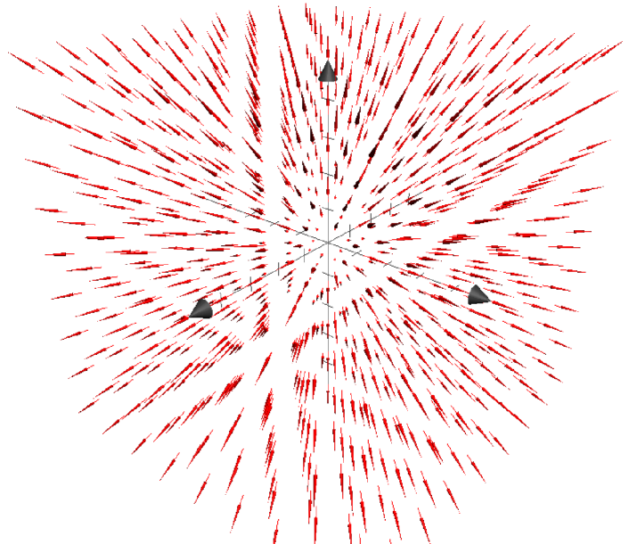
Figure 1. Plot of $\mathbf{F}=\nabla f$ for $f(x,y,z)=\sqrt{x^{2}+y^{2}+z^{2}}$

Relating Curls and Divergence

Let’s return to the second of our motivating questions. We’ll show the following:

$\mathbf{G}=\nabla\times\mathbf{F}$ is a curl if and only if the divergence $\nabla\cdot\mathbf{G}=0$.

First assume that $\mathbf{G}=\nabla\times\mathbf{F}$ for some $\mathbf{F}=M\,\mathbf{i}+N\,\mathbf{j}+P\,\mathbf{k}$. That is,

$$S\,\mathbf{i}+T\,\mathbf{j}+U\,\mathbf{k}=\left(\frac{\partial P}{\partial y}-\frac{\partial N}{\partial z}\right)\mathbf{i}+\left(\frac{\partial M}{\partial z}-\frac{\partial P}{\partial x}\right)\mathbf{j}+\left(\frac{\partial N}{\partial x}-\frac{\partial M}{\partial y}\right)\mathbf{k}.$$

We compute the divergence as

$$\nabla\cdot\mathbf{G} =\frac{\partial S}{\partial x}+\frac{\partial T}{\partial y}+\frac{\partial U}{\partial z}$$

$$=\left(\frac{\partial^{2}P}{\partial x\,\partial y}-\frac{\partial^{2}N}{\partial x\,\partial z}\right)+\left(\frac{\partial^{2}M}{\partial y\,\partial z}-\frac{\partial^{2}P}{\partial y\,\partial x}\right)+\left(\frac{\partial^{2}N}{\partial z\,\partial x}-\frac{\partial^{2}M}{\partial z\,\partial y}\right)$$

$$=0.$$

(Here, we assume that $M$, $N$, and $P$ are continuously twice-differentiable so that we can interchange the order of differentiation.)

Now what if $\nabla\cdot\mathbf{G}=0$? In this case, we write

$$\frac{\partial S}{\partial x}+\frac{\partial T}{\partial y}+\frac{\partial U}{\partial z}=0\qquad\implies\qquad U(x,y,z)=U(x,y,z_{0})-\int_{z_{0}}^{z}\left[\frac{\partial S}{\partial x}+\frac{\partial T}{\partial y}\right]d\zeta$$

for any fixed point $x_{0}\,\mathbf{i}+y_{0}\,\mathbf{j}+z_{0}\,\mathbf{k}\in D$. Define the function $\mathbf{F}=M\,\mathbf{i}+N\,\mathbf{j}+P\,\mathbf{k}$ in terms of the definite integrals

$$M(x,y,z) =\int_{z_{0}}^{z}T(x,y,\zeta)\,d\zeta-\int_{y_{0}}^{y}U(x,\tau,z_{0})\,d\tau$$

$$N(x,y,z) =-\int_{z_{0}}^{z}S(x,y,\zeta)\,d\zeta$$

$$P(x,y,z) =0.$$

Upon changing the order of differentiation and integration, we have the derivatives

$$\frac{\partial P}{\partial y}-\frac{\partial N}{\partial z} =S(x,y,z)$$

$$\frac{\partial M}{\partial z}-\frac{\partial P}{\partial x} =T(x,y,z)$$

$$\frac{\partial N}{\partial x}-\frac{\partial M}{\partial y} =U(x,y,z_{0})-\int_{z_{0}}^{z}\left[\frac{\partial S}{\partial x}+\frac{\partial T}{\partial y}\right]d\zeta=U(x,y,z).$$

It follows that $\nabla\times\mathbf{F}=\mathbf{G}$.

Exercise

Fix three real numbers $a$, $b$, and $c$ such that $a+b+c=0$, and define the function

$$\mathbf{G}=a\,x\,\mathbf{i}+b\,y\,\mathbf{j}+c\,z\,\mathbf{k}.$$

(See Figure 2 for a plot.) Show that $\nabla\cdot\mathbf{G}=0$. Moreover, find a function $\mathbf{F}$ such that $\mathbf{G}=\nabla\times\mathbf{F}$. (Hint: Guess a function in the form $\mathbf{F}=A\,y\,z\,\mathbf{i}+B\,x\,z\,\mathbf{j}+C\,x\,y\,\mathbf{k}$ for some real numbers $A$, $B$, and $C$.) How many such functions $\mathbf{F}$ do you think there are?

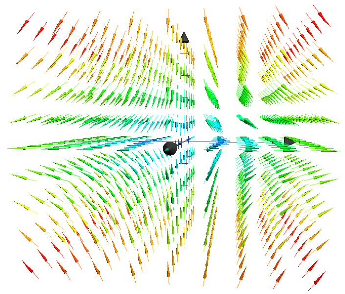
Figure 2. Plot of $\mathbf{G}=x\,\mathbf{i}+2\,y\,\mathbf{j}-3\,z\,\mathbf{k}$

Example

Consider the vector function

$$\mathbf{G}=\nabla f=\frac{x\,\mathbf{i}+y\,\mathbf{j}+z\,\mathbf{k}}{\sqrt{x^{2}+y^{2}+z^{2}}}\qquad\text{in terms of}\qquad f(x,y,z)=\sqrt{x^{2}+y^{2}+z^{2}}.$$

(Remember the “Prickly Pear”?) We will show that there is no vector potential $\mathbf{F}$ such that $\mathbf{G}=\nabla\times\mathbf{F}$. The idea is to show that the divergence of $\mathbf{G}$ is nonzero. To this end, we compute the higher-order partial derivatives using the Quotient Rule:

$$\frac{\partial^{2}f}{\partial x^{2}} =\frac{\partial}{\partial x}\left[\frac{x}{\sqrt{x^{2}+y^{2}+z^{2}}}\right]=\frac{y^{2}+z^{2}}{\left(x^{2}+y^{2}+z^{2}\right)^{3/2}}$$

$$\frac{\partial^{2}f}{\partial y^{2}} =\frac{\partial}{\partial y}\left[\frac{y}{\sqrt{x^{2}+y^{2}+z^{2}}}\right]=\frac{x^{2}+z^{2}}{\left(x^{2}+y^{2}+z^{2}\right)^{3/2}}$$

$$\frac{\partial^{2}f}{\partial z^{2}} =\frac{\partial}{\partial z}\left[\frac{z}{\sqrt{x^{2}+y^{2}+z^{2}}}\right]=\frac{x^{2}+y^{2}}{\left(x^{2}+y^{2}+z^{2}\right)^{3/2}}$$

(Check as an exercise!) Hence we find the divergence

$$\nabla\cdot\mathbf{G}=\frac{\partial^{2}f}{\partial x^{2}}+\frac{\partial^{2}f}{\partial y^{2}}+\frac{\partial^{2}f}{\partial z^{2}}=\frac{2\,x^{2}+2\,y^{2}+2\,z^{2}}{\left(x^{2}+y^{2}+z^{2}\right)^{3/2}}=\frac{2}{f}.$$

Since $\nabla\cdot\mathbf{G}\neq 0$, there cannot exist a function $\mathbf{F}$ such that $\mathbf{G}=\nabla\times\mathbf{F}$.

Differential Forms

Naturally, the three motivating questions in the introduction are rather naive questions to ask – although a bit difficult to answer! – so let’s make them a little more interesting. We’ll rephrase the definitions above in a way using differential $k$-forms; this will make integration more natural.

• A 0-form is a continuously differentiable function $f:D\to\mathbb{R}$. These are the functions we know and love from the one-variable Differential Calculus.
  

• A 1-form is an arc length differential in the form $\eta=M\,dx+N\,dy+P\,dz$ for some continuously differentiable vector field $\mathbf{F}:D\to\mathbb{R}^{3}$ in the form $\mathbf{F}=M\,\mathbf{i}+N\,\mathbf{j}+P\,\mathbf{k}$. Note that we can express this in the form $\eta=\mathbf{F}\cdot d\mathbf{r}$ using the dot product. We’ll use this to define path integrals later.
  

• A 2-form is an area differential in the form $\omega=S\,dy\,dz+T\,dx\,dz+U\,dx\,dy$ for some continuously differentiable vector field $\mathbf{G}:D\to\mathbb{R}^{3}$ in the form $\mathbf{G}=S\,\mathbf{i}+T\,\mathbf{j}+U\,\mathbf{k}$. Note that we can express this in the form $\omega=\mathbf{G}\cdot d\mathbf{A}$. As the notation suggests, we’ll use this to define surface integrals.
  

• 3-form is a volume differential in the form $\nu=f\,dx\,dy\,dz$ for some continuously differentiable function $f:D\to\mathbb{R}$. Note that we can express this in the form $\nu=f\,dV$. As the notation suggests, we’ll use this to define volume integrals.

We’ll denote $\Omega^{k}(D)$ as the collection of $k$-forms on $D$ for $k=0$, 1, 2, and 3. Boothby [2] provides a rigorous treatment of differential forms.

We claim that each $\Omega^{k}(D)$ these is a linear vector space. This means that the linear combination of two $k$-forms is another $k$-form. Consider, for example, 1-forms and 2-forms. Given scalars $\alpha$ and $\beta$, we have the identities

$$\left.\begin{aligned} \alpha\,&\bigl{(}M_{1}\,dx+N_{1}\,dy+P_{1}\,dz\bigr{)}+\beta\,\bigl{(}M_{2}\,dx+N_{2}\,dy+P_{2}\,dz\bigr{)}\\ &\qquad\qquad=\bigl{(}\alpha\,M_{1}+\beta\,M_{2}\bigr{)}\,dx+\bigl{(}\alpha\,N_{1}+\beta\,N_{2}\bigr{)}\,dy+\bigl{(}\alpha\,P_{1}+\beta\,P_{2}\bigr{)}\,dy\\[5.0pt] \alpha\,&\bigl{(}S_{1}\,dy\,dz+T_{1}\,dx\,dz+U_{1}\,dx\,dy\bigr{)}+\beta\,\bigl{(}S_{2}\,dy\,dz+T_{2}\,dx\,dz+U_{2}\,dx\,dy\bigr{)}\\ &\qquad\qquad=\bigl{(}\alpha\,S_{1}+\beta\,S_{2}\bigr{)}\,dy\,dz+\bigl{(}\alpha\,T_{1}+\beta\,T_{2}\bigr{)}\,dx\,dz+\bigl{(}\alpha\,U_{1}+\beta\,U_{2}\bigr{)}\,dx\,dy\end{aligned}\right.$$

Thus $\Omega^{k}(D)$ is a linear vector space for $k=1,2$. The argument for $k=0,3$ is similar.

Maps Between Differential Forms

How are these linear vector spaces related? Well, there are linear maps between them! Consider the following “differential” map $d:\Omega^{0}(D)\to\Omega^{1}(D)$ from 0-forms to 1-forms:

$$\begin{matrix}f\\[5.0pt] \downarrow\\[5.0pt] df=\dfrac{\partial f}{\partial x}\,dx+\dfrac{\partial f}{\partial y}\,dy+\dfrac{\partial f}{\partial z}\,dz=\nabla f\cdot d\mathbf{r}.\end{matrix}$$

This is linear because $d\bigl{(}\alpha\,f_{1}+\beta\,f_{2}\bigr{)}=\alpha\,df_{1}+\beta\,df_{2}$. Here, we write $d\mathbf{r}=dx\,\mathbf{i}+dy\,\mathbf{j}+dz\,\mathbf{k}$ as the arc length differential – expressed as a vector. Hence we find the answer to our first motivating question:

The vector-valued function $\mathbf{F}=\nabla f$ has a scalar potential $f$ if and only if the 1-form $\mathbf{F}\cdot d\mathbf{r}=df$ is the differential of some 0-form $f$.

Similarly, consider the following “differential” map $d:\Omega^{1}(D)\to\Omega^{2}(D)$ from 1-forms to 2-forms:

$$\begin{matrix}\eta=M\,dx+N\,dy+P\,dz=\mathbf{F}\cdot d\mathbf{r}\\[5.0pt] \downarrow\\[5.0pt] \begin{aligned} d\eta&=\left(\dfrac{\partial P}{\partial y}-\dfrac{\partial N}{\partial z}\right)dy\,dz+\left(\dfrac{\partial M}{\partial z}-\dfrac{\partial P}{\partial x}\right)dx\,dz+\left(\dfrac{\partial N}{\partial x}-\dfrac{\partial M}{\partial y}\right)dx\,dy\\ &=\bigl{(}\nabla\times\mathbf{F}\bigr{)}\cdot d\mathbf{A}.\end{aligned}\end{matrix}$$

This is linear because $d\bigl{(}\alpha\,\eta_{1}+\beta\,\eta_{2}\bigr{)}=\alpha\,d\eta_{1}+\beta\,d\eta_{2}$. Here, we write $d\mathbf{A}=dy\,dz\,\mathbf{i}+dx\,dz\,\mathbf{j}+dx\,dy\,\mathbf{k}$ as the area differential – also expressed as a vector. Hence we find the answer to our second motivating question:

The vector-valued function $\mathbf{G}=\nabla\times\mathbf{F}$ has a vector potential $\mathbf{F}$ if and only if the 2-form $\mathbf{G}\cdot d\mathbf{A}=d\eta$ is the differential of some 1-form $\eta=\mathbf{F}\cdot d\mathbf{r}$.

Recall that $\mathbf{F}=\nabla f$ is a gradient if and only if the curl $\nabla\times\mathbf{F}=\mathbf{0}$. In other words, given a 1-form $\eta=M\,dx+N\,dy+P\,dz=\mathbf{F}\cdot d\mathbf{r}$, we have $\eta=df$ as the differential of a 0-form if and only if the 2-form $d\eta=0$. This is yet another answer to our first question!

Finally, consider the following “differential” map $d:\Omega^{2}(D)\to\Omega^{3}(D)$ from 2-forms to 3-forms:

$$\begin{matrix}\omega=S\,dy\,dz+T\,dx\,dz+U\,dx\,dy=\mathbf{G}\cdot d\mathbf{A}\\[5.0pt] \downarrow\\[5.0pt] d\omega=\left(\dfrac{\partial S}{\partial x}+\dfrac{\partial T}{\partial y}+\dfrac{\partial U}{\partial z}\right)dx\,dy\,dz=\bigl{(}\nabla\cdot\mathbf{G}\bigr{)}\,dV.\end{matrix}$$

Again, this is linear because $d\bigl{(}\alpha\,\omega_{1}+\beta\,\omega_{2}\bigr{)}=\alpha\,d\omega_{1}+\beta\,d\omega_{2}$. Remember that $dV=dx\,dy\,dz$ is the volume differential. Hence we find the answer to the last of our three motivating questions:

The vector-valued function $f=\nabla\cdot\mathbf{G}$ has a vector potential $\mathbf{G}$ if and only if the 3-form $f\,dV=d\omega$ is the differential of some 2-form $\omega=\mathbf{G}\cdot d\mathbf{A}$.

Recall that $\mathbf{G}=\nabla\times\mathbf{F}$ is a curl if and only if the divergence $\nabla\cdot\mathbf{G}=0$. In other words, given a 2-form $\omega=S\,dy\,dz+T\,dx\,dz+U\,dx\,dy=\mathbf{G}\cdot d\mathbf{A}$, we have $\omega=d\eta$ as the differential of a 1-form if and only if the 3-form $d\omega=0$. This is yet another answer to our second question!

We’ll summarize this via the following diagram of maps:

$$\setcounter{MaxMatrixCols}{11}\begin{CD}\{0\}@>{}>{}>\Omega^{0}(D)@>{\text{gradient}}>{}>\Omega^{1}(D)@>{\text{curl}}>{}>\Omega^{2}(D)@>{\text{divergence}}>{}>\Omega^{3}(D)@>{}>{}>\{0\}.\end{CD}$$

All of the various definitions of differentiation for functions in three variables are all related via linear transformations on the vector spaces of $k$-forms!

Example

Let’s consider the differential 1-form

$$\eta=y\,z\,dx+x\,z\,dy+x\,y\,dz.$$

This is in the form $M\,dx+N\,dy+P\,dz$ for $M=y\,z$, $N=x\,z$, and $P=x\,y$. (See Figure 3 for a plot of $\mathbf{F}=M\,\mathbf{i}+N\,\mathbf{j}+P\,\mathbf{k}$.) We’ll compute the differential $d\eta$. We have the partial derivatives

$$\dfrac{\partial P}{\partial y}-\dfrac{\partial N}{\partial z}=x-x=0,\quad\dfrac{\partial M}{\partial z}-\dfrac{\partial P}{\partial x}=y-y=0,\quad\dfrac{\partial N}{\partial x}-\dfrac{\partial M}{\partial y}=z-z=0.$$

Hence $d\eta=0$.

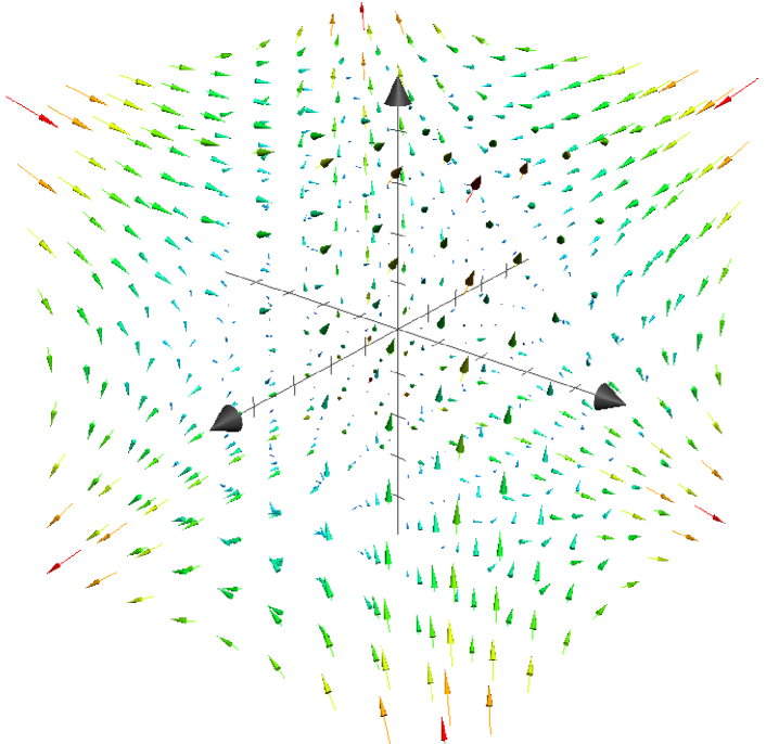
Figure 3. Plot of $\mathbf{F}=y\,z\,\mathbf{i}+x\,z\,\mathbf{j}+x\,y\,\mathbf{k}$

Exercise

Fix three real numbers $a$, $b$, and $c$ such that $a+b+c=0$, and differential 2-form

$$\omega=a\,x\,dy\,dz+b\,y\,dx\,dz+c\,z\,dx\,dy.$$

Show that $\omega=d\eta$ is the differential of the 1-form $\eta=b\,y\,z\,dx-a\,x\,z\,dy$. Is this the only 1-form $\eta$ such that $\omega=d\eta$?

Integration

We know now how the various forms of differentiation are all related, but what about integration? First, we review what we mean by integration. As $D\subseteq\mathbb{R}^{3}$ is a subset of three-dimensional space, we can define integration for one variable, two variables, or even three variables.

Fundamental Theorem of Calculus

In order to define an integral for one variable, let $\mathbf{r}:I\to D$ be a continuously differentiable map, which we write in the form $\mathbf{r}=x\,\mathbf{i}+y\,\mathbf{j}+z\,\mathbf{k}$, defined on a closed interval $I=[a,b]$. We say that the image $C\subseteq D$ is a path. Given vector field $\mathbf{F}:D\to\mathbb{R}^{3}$, the composition gives the 1-form $\eta=\mathbf{F}\bigl{(}\mathbf{r}(t)\bigr{)}\cdot d\mathbf{r}$, so naturally a path integral as

$$\int_{C}\eta=\int_{a}^{b}\left[M\bigl{(}\mathbf{r}(t)\bigr{)}\,\frac{dx}{dt}+N\bigl{(}\mathbf{r}(t)\bigr{)}\,\frac{dy}{dt}+P\bigl{(}\mathbf{r}(t)\bigr{)}\,\frac{dz}{dt}\right]dt.$$

Recall that $\mathbf{F}=\nabla f$ has a scalar potential $f$ if and only if $\eta=df$ is the differential of a 0-form $f$. In this case, the path integral simplifies to

$$\int_{a}^{b}\frac{d}{dt}\biggl{[}f\bigl{(}\mathbf{r}(t)\bigr{)}\biggr{]}dt=\int_{C}df=f(\mathbf{r})\biggr{|}_{\partial C}=f\bigl{(}\mathbf{r}(b)\bigr{)}-f\bigl{(}\mathbf{r}(a)\bigr{)}.$$

Hence the integral is independent of the path $C$, and it is only dependent on the endpoints $\partial C=\left\{\mathbf{r}(a),\ \mathbf{r}(b)\right\}$. This is just the Fundamental Theorem of Calculus.

Example

Let $D=\mathbb{R}^{3}$ be all of three-dimensional space, and let $C$ denote the circle of radius $r$ in the plane. Note that $C$ is the set of points $x\,\mathbf{i}+y\,\mathbf{j}+z\,\mathbf{k}$ such that $x^{2}+y^{2}=r^{2}$ and $z=0$. We may think of this as being the image of the map $\mathbf{r}:[0,2\pi]\to\mathbb{R}^{3}$ which sends $t\mapsto r\,\cos t\,\mathbf{i}+r\,\sin t\,\mathbf{j}$. The circle is just an example of a path!

Now let’s consider a vector field $\mathbf{F}=-(y/2)\,\mathbf{i}+(x/2)\,\mathbf{j}$. (See Figure 4 for a plot.) We’ll explain why there does not exist a scalar function $f$ such that $\mathbf{F}=\nabla f$. The idea is to suppose that $f$ does indeed exist and then compute the integral of $\mathbf{F}$ around the path $C$. Let’s consider the following differential 1-form:

$$\eta =\mathbf{F}\bigl{(}\mathbf{r}(t)\bigr{)}\cdot d\mathbf{r}=\biggl{(}-\frac{r\,\cos t}{2}\,\mathbf{i}+\frac{r\,\sin t}{2}\,\mathbf{j}\biggr{)}\cdot\biggl{(}-r\,\cos t\,dt\,\mathbf{i}+r\,\sin t\,dt\,\mathbf{j}\biggr{)}$$

$$=\frac{r^{2}\,\cos^{2}t\,dt+r^{2}\,\sin^{2}t\,dt}{2}=\frac{r^{2}}{2}\,dt.$$

If $\mathbf{F}=\nabla f$, then $\int_{C}\eta=f\bigl{(}\mathbf{r}(2\pi)\bigr{)}-f\bigl{(}\mathbf{r}(0)\bigr{)}=0.$ But actually,

$$\int_{C}\eta=\int_{0}^{2\pi}\frac{r^{2}}{2}\,dt=\pi\,r^{2}.$$

Hence there is no function $f$ such that $\mathbf{F}=\nabla f$. (Of course, we could have seen this sooner by computing the curl $\nabla\times\mathbf{F}=\mathbf{k}$ and realizing it’s a nonzero vector.)

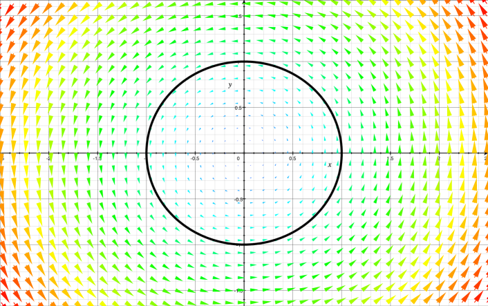
Figure 4. Plot of $\mathbf{F}=-(y/2)\,\mathbf{i}+(x/2)\,\mathbf{j}$

Stokes’ Theorem and Green’s Theorem

In order to define an integral for two variables, let $\mathbf{r}:R\to D$ be a continuously differentiable map, which we write in the form $\mathbf{r}=x\,\mathbf{i}+y\,\mathbf{j}+z\,\mathbf{k}$, that is defined on an closed region $R=[a,b]\times[c,d]$. We say that the image $S\subseteq D$ is a surface, and assume that its boundary $C=\partial S$ is a curve as before. Given vector field $\mathbf{G}:D\to\mathbb{R}^{3}$, the composition gives the 2-form $\omega=\mathbf{G}\bigl{(}\mathbf{r}(u,v)\bigr{)}\cdot d\mathbf{A}$, so naturally surface integral is defined as

$$\iint_{S}\omega=\int_{a}^{b}\int_{c}^{d}\left|\begin{matrix}S\bigl{(}\mathbf{r}(u,v)\bigr{)}&T\bigl{(}\mathbf{r}(u,v)\bigr{)}&U\bigl{(}\mathbf{r}(u,v)\bigr{)}\\[8.0pt] \dfrac{\partial x}{\partial u}&\dfrac{\partial y}{\partial u}&\dfrac{\partial z}{\partial u}\\[8.0pt] \dfrac{\partial x}{\partial v}&\dfrac{\partial y}{\partial v}&\dfrac{\partial z}{\partial v}\end{matrix}\right|du\,dv.$$

Recall that $\mathbf{G}=\nabla\times\mathbf{F}$ has a vector potential $\mathbf{F}$ if and only if $\omega=d\eta$ is the differential of a 1-form $\eta$. In this case, the surface integral simplifies to

$$\iint_{S}\bigl{(}\nabla\times\mathbf{F}\bigr{)}\cdot d\mathbf{A}=\iint_{S}d\eta=\int_{\partial S}\eta=\int_{C}\mathbf{F}\cdot d\mathbf{r}.$$

Hence the integral is independent of the surface $\mathcal{S}$, and it is only dependent on the boundary $C=\partial S$. This is known as Stokes’ Theorem.

Let’s consider a special case, where $\mathbf{r}:R\to\mathbb{R}^{2}$ actually maps into the plane. Then $S\subseteq\mathbb{R}^{2}$, so write $\mathbf{F}=M\,\mathbf{i}+N\,\mathbf{j}$. Stokes’ Theorem in the plane reduces to the statement

$$\iint_{S}\left(\frac{\partial N}{\partial x}-\frac{\partial M}{\partial y}\right)dx\,dy=\iint_{S}d\eta=\int_{\partial R}\eta=\int_{\partial S}\bigl{[}M\,dx+N\,dy\bigr{]}.$$

This is known as Green’s Theorem. Similarly, for the orthogonal vector field $\mathbf{F}_{\perp}=-N\,\mathbf{i}+M\,\mathbf{j}$, the Divergence Theorem in the Plane is the expression

$$\iint_{S}\left(\frac{\partial M}{\partial x}+\frac{\partial N}{\partial y}\right)dx\,dy=\int_{\partial S}\bigl{[}-N\,dx+M\,dy\bigr{]}.$$

Example

Let $D=\mathbb{R}^{3}$ be all of three-dimensional space, and let $S$ denote the disk of radius $r$ in the plane. The latter is just the set of points $x\,\mathbf{i}+y\,\mathbf{j}+z\,\mathbf{k}$ such that $x^{2}+y^{2}\leq r^{2}$ and $z=0$. We may think of this as being the image of the map $\mathbf{r}:[0,r]\times[0,2\pi]\to\mathbb{R}^{3}$ which sends $(\rho,\theta)\mapsto\rho\,\cos\theta\,\mathbf{i}+\rho\,\sin\theta\,\mathbf{j}$. Note that the boundary $C=\partial S$ is simply the circle $x^{2}+y^{2}=r^{2}$, which we considered before.

Let’s return to the vector field $\mathbf{F}=-(y/2)\,\mathbf{i}+(x/2)\,\mathbf{j}$. We’ll consider the differential 2-form $\omega=\bigl{(}\nabla\times\mathbf{F}\bigr{)}\cdot d\mathbf{A}=\mathbf{k}\cdot d\mathbf{A}=dx\,dy$. Stokes’ Theorem (or really Green’s Theorem, since it’s in the plane) states that

$$\iint_{S}\omega=\int_{C}\mathbf{F}\cdot d\mathbf{r}=\pi\,r^{2}.$$

(Recall the previous example.) Let’s compute the integral on the left-hand side in a different way. This differential 2-form can also expressed in polar coordinates using the determinant

$$\omega =\left|\begin{matrix}S\bigl{(}\mathbf{r}(\rho,\theta)\bigr{)}&T\bigl{(}\mathbf{r}(\rho,\theta)\bigr{)}&U\bigl{(}\mathbf{r}(\rho,\theta)\bigr{)}\\[8.0pt] \dfrac{\partial x}{\partial\rho}&\dfrac{\partial y}{\partial\rho}&\dfrac{\partial z}{\partial\rho}\\[8.0pt] \dfrac{\partial x}{\partial\theta}&\dfrac{\partial y}{\partial\theta}&\dfrac{\partial z}{\partial\theta}\end{matrix}\right|d\rho\,d\theta=\left|\begin{matrix}0&0&1\\ \cos\theta&\sin\theta&0\\ -\rho\,\sin\theta&\rho\,\cos\theta&0\end{matrix}\right|d\rho\,d\theta$$

$$=\rho\,d\rho\,d\theta.$$

Hence we have the integral

$$\iint_{S}dx\,dy=\iint_{S}\omega=\int_{0}^{r}\int_{0}^{2\pi}\rho\,d\rho\,d\theta=\left[\int_{0}^{r}\rho\,d\rho\right]\left[\int_{0}^{2\pi}d\theta\right]=\pi\,r^{2}.$$

Of course, this is just the area of the disk $S$.

Exercise

Let $S$ be any surface in the plane $\mathbb{R}^{2}$ with a boundary $C=\partial S$. Show that its area can be computed using a path integral around along $C$. That is,

$$\text{Area}(S)=\iint_{S}dx\,dy=\int_{C}\frac{-y\,dx+x\,dy}{2}.$$

Gauss’ Theorem and the Divergence Theorem.

In order to define an integral for three variables, let $\mathbf{r}:B\to\mathbb{R}^{3}$ be a continuously differentiable map, which we write in the form $\mathbf{r}=x\,\mathbf{i}+y\,\mathbf{j}+z\,\mathbf{k}$, defined on an closed region $B=[a,b]\times[c,d]\times[p,q]$. We say that the image $D\subseteq\mathbb{R}^{3}$ is a region, and assume that its boundary $S=\partial D$ is a surface as before. Given a scalar function $f:D\to\mathbb{R}$, the composition gives the differential 3-form $\nu=f\bigl{(}\mathbf{r}(u,v,w)\bigr{)}\,dV$, so naturally define a volume integral as

$$\iiint_{D}\nu=\int_{a}^{b}\int_{c}^{d}\int_{p}^{q}f\bigl{(}\mathbf{r}(u,v,w)\bigr{)}\left|\begin{matrix}\dfrac{\partial x}{\partial u}&\dfrac{\partial y}{\partial u}&\dfrac{\partial z}{\partial u}\\[8.0pt] \dfrac{\partial x}{\partial v}&\dfrac{\partial y}{\partial v}&\dfrac{\partial z}{\partial v}\\[8.0pt] \dfrac{\partial x}{\partial w}&\dfrac{\partial y}{\partial w}&\dfrac{\partial z}{\partial w}\end{matrix}\right|du\,dv\,dw.$$

(As with surface integrals, we’ve expressed the integrand above using a $3\times 3$ determinant. Most texts refer to this as the Jacobian of the transformation $\mathbf{r}:B\to D$.) Recall that $f=\nabla\cdot\mathbf{G}$ has a vector potential $\mathbf{G}$ if and only if $\nu=d\omega$ is a differential of a 2-form $\omega$. In this case, the volume integral simplifies to

$$\iiint_{D}\bigl{(}\nabla\cdot\mathbf{G}\bigr{)}\,dV=\iiint_{D}d\omega=\iint_{\partial D}\omega=\iint_{S}\mathbf{G}\cdot d\mathbf{A}.$$

Hence the integral is independent of the region $V$, and it is only dependent on the boundary $S=\partial D$. This is known as Gauss’ Theorem, or the Divergence Theorem.

Example

Let $D$ denote the solid sphere of radius $r$ in three-dimensional space. This is just the set of points $x\,\mathbf{i}+y\,\mathbf{j}+z\,\mathbf{k}$ such that $x^{2}+y^{2}+z^{2}\leq r^{2}$. We may think of this as being the image of the map $\mathbf{r}:[0,r]\times[0,\pi]\times[0,2\pi]\to\mathbb{R}^{3}$ which sends

$$(\rho,\phi,\theta)\mapsto\rho\,\sin\phi\,\cos\theta\,\mathbf{i}+\rho\,\sin\phi\,\sin\theta\,\mathbf{j}+\rho\,\cos\phi\,\mathbf{k}.$$

Note that the boundary $S=\partial D$ is simply the sphere $x^{2}+y^{2}+z^{2}=r^{2}$.

Let’s return to the vector field

$$\mathbf{G}=\nabla g=\frac{x\,\mathbf{i}+y\,\mathbf{j}+z\,\mathbf{k}}{\sqrt{x^{2}+y^{2}+z^{2}}}\qquad\text{in terms of}\qquad g(x,y,z)=\sqrt{x^{2}+y^{2}+z^{2}}.$$

(The “Prickly Pear” again!) We will compute integrals and verify the Divergence Theorem. We may express the volume element $dV=dx\,dy\,dz$ in spherical coordinates using the determinant

$$dV =\left|\begin{matrix}\dfrac{\partial x}{\partial\rho}&\dfrac{\partial y}{\partial\rho}&\dfrac{\partial z}{\partial\rho}\\[8.0pt] \dfrac{\partial x}{\partial\phi}&\dfrac{\partial y}{\partial\phi}&\dfrac{\partial z}{\partial\phi}\\[8.0pt] \dfrac{\partial x}{\partial\theta}&\dfrac{\partial y}{\partial\theta}&\dfrac{\partial z}{\partial\theta}\end{matrix}\right|d\rho\,d\phi\,d\theta=\left|\begin{matrix}\cos\theta\,\sin\phi&\sin\theta\,\sin\phi&\cos\phi\\[5.0pt] \rho\,\cos\theta\,\cos\phi&\rho\,\sin\theta\,\cos\phi&-\rho\,\sin\phi\\[5.0pt] -\rho\,\sin\theta\,\sin\phi&\rho\,\cos\theta\,\sin\phi&0\end{matrix}\right|d\rho\,d\phi\,d\theta$$

$$=\rho^{2}\,\sin\phi\,d\rho\,d\phi\,d\theta.$$

Hence we have the differential 3-form

$$\nu=\nabla\cdot\mathbf{G}\bigr{(}\mathbf{r}(\rho,\phi,\theta)\bigl{)}\,dV=\frac{2}{\rho}\cdot\bigl{(}\rho^{2}\,\sin\phi\,d\rho\,d\phi\,d\theta\bigr{)}=2\,\rho\,\sin\phi\,d\rho\,d\phi\,d\theta.$$

(Recall that $\nabla\cdot\mathbf{G}=2/g$.) This gives the integral

$$\iiint_{D}\nu =\int_{0}^{r}\int_{0}^{\pi}\int_{0}^{2\pi}2\,\rho\,\sin\phi\,d\rho\,d\phi\,d\theta=\left[\int_{0}^{r}2\,\rho\,d\rho\right]\left[\int_{0}^{\pi}\sin\phi\,d\phi\right]\left[\int_{0}^{2\pi}d\theta\right]$$

$$=4\,\pi\,r^{2}.$$

On the other hand, we may express the area element is the determinant

$$d\mathbf{A} =\left|\begin{matrix}\mathbf{i}&\mathbf{j}&\mathbf{k}\\[8.0pt] \dfrac{\partial x}{\partial\phi}&\dfrac{\partial y}{\partial\phi}&\dfrac{\partial z}{\partial\phi}\\[8.0pt] \dfrac{\partial x}{\partial\theta}&\dfrac{\partial y}{\partial\theta}&\dfrac{\partial z}{\partial\theta}\end{matrix}\right|d\phi\,d\theta=\left|\begin{matrix}\mathbf{i}&\mathbf{j}&\mathbf{k}\\[5.0pt] \rho\,\cos\theta\,\cos\phi&\rho\,\sin\theta\,\cos\phi&-\rho\,\sin\phi\\[5.0pt] -\rho\,\sin\theta\,\sin\phi&\rho\,\cos\theta\,\sin\phi&0\end{matrix}\right|d\phi\,d\theta$$

$$=\rho\,\sin\phi\,\bigl{(}\rho\,\sin\phi\,\cos\theta\,\mathbf{i}+\rho\,\sin\phi\,\sin\theta\,\mathbf{j}+\rho\,\cos\phi\,\mathbf{k}\bigr{)}\,d\phi\,d\theta.$$

Hence we have the differential 2-form

$$\omega=\mathbf{G}\bigl{(}\mathbf{r}(\rho,\phi,\theta)\bigr{)}\cdot d\mathbf{A}=\frac{\mathbf{r}}{\rho}\cdot\bigl{(}\rho\,\sin\phi\,\mathbf{r}\,d\theta\,d\phi\bigr{)}=\rho^{2}\,\sin\phi\,d\phi\,d\theta.$$

This gives the integral

$$\iint_{\partial D}\omega=\int_{0}^{\pi}\int_{0}^{2\pi}r^{2}\,\sin\phi\,d\theta\,d\phi=r^{2}\left[\int_{0}^{\pi}\sin\phi\,d\phi\right]\left[\int_{0}^{2\pi}d\theta\right]=4\,\pi\,r^{2}.$$

(Remember that $\rho=r$ along the boundary $S=\partial D$.) This indeed verifies that

$$\iiint_{D}\bigl{(}\nabla\cdot\mathbf{G}\bigr{)}\,dV=\iint_{S}\mathbf{G}\cdot d\mathbf{A}.$$

Arfken and Weber [1] provides a plethora of formulas for integrating in different coordinate systems other than spherical.

Exercise

Let $D$ be any region in $\mathbb{R}^{3}$ with a boundary $S=\partial D$. Show that its volume can be computed using a surface integral on $S$. That is,

$$\text{Vol}(D)=\iiint_{D}dx\,dy\,dz=\iint_{S}\frac{x\,dy\,dz+y\,dx\,dz+z\,dx\,dy}{3}.$$

The Moral of the Story

In this paper we have shown that all of the theorems – those for differentiation and integration – can be expressed using differential forms. Here’s the idea in a nutshell for any region $D$. We consider a series of linear vector spaces $\Omega^{k}(D)$, where we have “differential” maps

$$\begin{CD}\cdots @>{}>{}>\Omega^{k-1}(D)@>{d}>{}>\Omega^{k}(D)@>{d}>{}>\Omega^{k+1}(D)@>{}>{}>\cdots\end{CD}$$

We would like to know the answer to the following question involving differentiation:

Which $k$-forms $\omega\in\Omega^{k+1}(D)$ are in the form
$\omega=d\eta$ for some $(k-1)$-form $\eta\in\Omega^{k}(D)$?

The partial answer should be:

If $\omega=d\eta$ for some $(k-1)$-form $\eta$,
then $d\omega=0$ as a $(k+1)$-form.

A complete answer involves computing something called de Rham Cohomology. (The desert after the Main Course?) For instance, we have computed de Rham Cohomlogy in this article for certain subsets of three-dimensional space. We expect to generalize the integration formulas above by saying something like

$$\int_{D}\omega=\int_{D}d\eta=\int_{\partial D}\eta$$

so that the integral would be independent of the region $D$, and would be only dependent on the boundary $\partial D$. This is the Generalized Stokes’ Theorem. Surprisingly, this entire theory can be worked out for “many” sets $D$. But don’t take our words for it – just a friendly Differential Geometer!

Appendix: $3\times 3$ Determinants

A $3\times 3$ determinant is the quantity

$$\left|\begin{tabular}[]{ccc}$a_{11}$&$a_{12}$&$a_{13}$\\ $a_{21}$&$a_{22}$&$a_{23}$\\ $a_{31}$&$a_{32}$&$a_{33}$\end{tabular}\right|=\begin{aligned} a_{11}(\,a_{22}\,a_{33}&-a_{23}\,a_{32})-a_{12}(\,a_{23}\,a_{31}-\,a_{21}\,a_{33})\\ &+a_{13}(\,a_{21}\,a_{32}-a_{22}\,a_{31}).\end{aligned}$$

Another way is to compute the determinant is by using the following diagram:

Here we multiply along the arrows, then add or subtract depending on the direction of the arrow:

$$\left|\begin{tabular}[]{ccc}$a_{11}$&$a_{12}$&$a_{13}$\\ $a_{21}$&$a_{22}$&$a_{23}$\\ $a_{31}$&$a_{32}$&$a_{33}$\end{tabular}\right|=\begin{aligned} &\left(a_{11}\,a_{22}\,a_{33}+a_{12}\,a_{23}\,a_{31}+a_{13}\,a_{21}\,a_{32}\right)\\ &\quad\qquad\qquad-\left(a_{11}\,a_{23}\,a_{32}+a_{12}\,a_{21}\,a_{33}+a_{13}\,a_{22}\,a_{31}\right).\end{aligned}$$

References

- [1] George B. Arfken and Hans J. Weber. Mathematical methods for physicists. Harcourt/Academic Press, Burlington, MA, fifth edition, 2001.
- [2] William M. Boothby. An introduction to differentiable manifolds and Riemannian geometry, volume 120 of Pure and Applied Mathematics. Academic Press Inc., Orlando, FL, second edition, 1986.
- [3] Deborah Hughes-Hallett, Andrew M. Gleason, William G. McCallum, Daniel E. Flath, Patti Frazer Lock, Thomas W. Tucker, David O. Lomen, David Lovelock, David Mumford, Brad G. Osgood, Douglas Quinney, Karen Rhea, and Jeff Tecosky-Feldman. Calculus: Single and Multivariable. Wiley-Interscience [John Wiley & Sons], 4th edition, December 2004.
- [4] Ron Larson, Robert P. Hostetler, and Bruce H. Edwards. Calculus: Early Transcendental Functions. Houghton Mifflin, fourth edition, 2007.
- [5] Jerrold E. Marsden and Anthony J. Tromba. Vector Calculus. W. H. Freeman, 5th edition, 2004.
- [6] James Stewart. Calculus: Early Transcendentals, volume 6E of Calculus. Brooks Cole, 2008.