Pionic BEC–BCS crossover at finite isospin chemical potential

Abstract

We study the character change of the pionic condensation at finite isospin chemical potential $\mu_{\mathrm{I}}$ by adopting the linear sigma model as a non-local interaction between quarks. At low $|\mu_{\mathrm{I}}|$ the condensation is purely bosonic, then the Cooper pairing around the Fermi surface grows gradually as $|\mu_{\mathrm{I}}|$ increases. This $q$-$\bar{q}$ pairing is weakly coupled in comparison with the case of the $q$-$q$ pairing that leads to color superconductivity.

Recent progress in computer power makes it possible to reliably simulate quantum chromodynamics (QCD) at finite temperature $T$. As for finite density (usually parametrized by finite baryon chemical potential $\mu_{\mathrm{B}}$), however, the well known sign problem limits simulations. Alternatively, QCD at finite isospin chemical potential $\mu_{\mathrm{I}}=\mu_{u}-\mu_{d}$ (where $\mu_{u}$ and $\mu_{d}$ denoting the chemical potential of $u$ and $d$ quark, respectively) as well as the SU(2) color systems, in which the sign problem does not exist, are studied to give insights into the actual finite $\mu_{\mathrm{B}}$ physics J. B. Kogut and D. K. Sinclair (2002a). These systems are also studied extensively in terms of effective models M. Frank et al. (2003); Y. Nishida (2004); A. Barducci et al. (2004); M. Loewe and C. Villavicencio (2005); S. Mukherjee et al. (2007); Z. Zhang and Y.-X. Liu (2007); J. O. Andersen and T. Brauner (2008). One of the most interesting aspects of the finite $\mu_{\mathrm{I}}$ systems is that they accommodate pion condensation for $|\mu_{\mathrm{I}}|>m_{\pi}$ D. K. Campbell et al. (1975), with $m_{\pi}$ denoting the mass of pions. Son and Stephanov D. T. Son and M. A. Stephanov (2001) predicted that the pion condensed phase evolves to Cooper pairing between $u$ and $\bar{d}$ ($d$ and $\bar{u}$) for $\mu_{\mathrm{I}}>0$ ($<0$) at high $|\mu_{\mathrm{I}}|$, but the quantitative process of the character change of the condensation has not been discussed.

The BEC–BCS crossover has long been expected to occur in various quantum systems A. J. Leggett (1980); P. Nozières and S. Schmitt-Rink (1985); H. E. Haber and H. A. Weldon (1982); it was experimentally observed in ultra cold atomic gases, in which the strength of the interaction can be tuned artificially, only recently. At least in principle, it can occur also in systems governed by the strong interaction, in which the strength of the interaction can not be tuned artificially aside from theoretical simulations Y. Nishida and H. Abuki (2005). Rather, the change in the environment, typically density, would lead to the crossover G. Sun et al. (2007). In symmetric nuclear matter, the neutron ($n$)–proton ($p$) pairing in the ${}^{3}S_{1}$ + ${}^{3}D_{1}$ channel that leads to bound deuteron formation was studied in Ref. M. Baldo et al. (1995). The $n$–$n$ and $p$–$p$ ${}^{1}S_{0}$ pairing, that has attracted attention from viewpoints of both nuclear structure and neutron stars, however, does not reach the BEC T. Tanigawa and M. Matsuzaki (1999); M. Matsuo (2006). In intermediate density quark matter, the present author discussed that the spatial extension of quark Cooper pairs in a color superconductor is comparable with the mean interparticle distance M. Matsuzaki (2000). Later, a wide enough density region was studied H. Abuki et al. (2002) and it was shown that the diquark pairing becomes weak at extremely high density. The properties of the pseudo gap phase and bosonic excitations were studied in Refs. M. Kitazawa et al. (2004); P. Castorina et al. (2005); T. Brauner (2008).

Since the mechanism of the fermion-antifermion condensation that produces the fermion mass is essentially the same as the BCS pairing as recognized in Nambu and Jona-Lasinio’s celebrated paper Y. Nambu and G. Jona-Lasinio (1961), the evolution of the charged pion condensation to $q$–$\bar{q}$ Cooper pairs can be analyzed in the context of the BEC–BCS crossover in terms of the spatial structure of the pion condensation. To this end, one must introduce a non-local interaction between $q$ and $\bar{q}$ that gives momentum dependent condensations. In the present study, we adopt the linear sigma model M. Gell-Mann and M. Lèvy (1960), which respects chiral symmetry, as an inter-quark interaction, since 1) the pion condensation occurs as a spontaneous symmetry breaking among three pions that have light but non-zero masses after the chiral symmetry breaking between the sigma meson and the pions, and 2) the effect of high $|\mu_{\mathrm{I}}|$ on it has long been studied D. K. Campbell et al. (1975); L. He et al. (2005); H. Mao et al. (2006); J. O. Andersen (2007). In Ref. J. Deng et al. (2007) the BEC–BCS crossover in the diquark pairing was studied in a boson–fermion model similar to that of the present study but the condensation is momentum independent.

Finite $\mu_{\mathrm{I}}$ occurs with finite $\mu_{\mathrm{B}}$ in the real world; with finite $T$ and small $\mu_{\mathrm{B}}$, for example 0.04 GeV W. Broniowski and W. Florkowski (2001), in heavy ion collisions and with (near) zero $T$ and large $\mu_{\mathrm{B}}$, for example $\gtrsim$ 1 GeV, in compact stars. In this sense, the present study of the system with $\mu_{\mathrm{B}}=0$ is just the first step to investigate the realistic systems. However, since a signature of the BEC–BCS crossover in the chemical potential dependence of the condensation is measured in a lattice simulation for the SU(2) color system S. Hands et al. (2005) that is in a sense dual J. B. Kogut and D. K. Sinclair (2002b) to the finite $\mu_{\mathrm{I}}$ system, the spatial structure of the composite pions would be worth studying even with $\mu_{\mathrm{B}}=0$.

When a conserved charge density $\mathcal{N}$ exists, the effective Lagrangian density is obtained with replacing the Hamiltonian density $\mathcal{H}$ by $\mathcal{H}-\mu\mathcal{N}$, here $\mu$ denoting the corresponding chemical potential, in the partition function and performing momentum-field integrations J. I. Kapusta (1989). The result for the charged pion is

$$\mathcal{L}_{\mathrm{eff}}=\mathcal{L}(\dot{\pi_{1}}\rightarrow\dot{\pi_{1}}-\mu\pi_{2},\dot{\pi_{2}}\rightarrow\dot{\pi_{2}}+\mu\pi_{1}).$$ (1)

Since the isospin chemical potential $\mu_{\mathrm{I}}$ corresponds to the charge chemical potential in the hadronic world, this form applies to the present purpose. This indicates that the role of $\mu_{\mathrm{I}}$ corresponds to that of the angular frequency in the non-relativistic spatial rotation, that is, to move to a “coordinate frame” rotating in the 3 dimensional isospin space; the zero-energy rotational motion is a physical image of the Nambu–Goldstone mode.

The adopted effective Lagrangian for the quarks, sigma mesons and pions is

$$\mathcal{L}_{\mathrm{eff}}=\mathcal{L}_{\mathrm{q}}+\mathcal{L}_{\mathrm{M}}+\mathcal{L}_{\mathrm{couple}},$$

$$\mathcal{L}_{\mathrm{q}}=\bar{q}(i\ooalign{\hfil/\hfil\crcr$\partial$}-m_{q}+\frac{\mu_{\mathrm{I}}}{2}\gamma^{0}\tau_{3})q,$$ (4)

$$\mathcal{L}_{\mathrm{M}}=\frac{1}{2}(\partial_{\mu}\sigma\partial^{\mu}\sigma+\partial_{\mu}\overrightarrow{\pi}\cdot\partial^{\mu}\overrightarrow{\pi})-U(\sigma,\overrightarrow{\pi})$$

$$+\mu_{\mathrm{I}}(\pi_{1}\dot{\pi_{2}}-\pi_{2}\dot{\pi_{1}})+\frac{\mu_{\mathrm{I}}^{2}}{2}(\pi_{1}^{2}+\pi_{2}^{2}),$$

$$U(\sigma,\overrightarrow{\pi})=\frac{\lambda^{2}}{4}(\sigma^{2}+\overrightarrow{\pi}^{2})^{2}-\frac{m_{0}^{2}}{2}(\sigma^{2}+\overrightarrow{\pi}^{2})-c\sigma,$$

$$m_{0}^{2}=\lambda^{2}f_{\pi}^{2}-m_{\pi}^{2}\quad(>0),\quad c=f_{\pi}m_{\pi}^{2},$$

$$\mathcal{L}_{\mathrm{couple}}=-G\bar{q}(\sigma+i\gamma^{5}\overrightarrow{\tau}\cdot\overrightarrow{\pi})q,$$ (5)

where $f_{\pi}$ and $m_{\pi}$ stand for the pion decay constant and the pion mass, respectively. Hereafter, quantum fluctuations are indicated by primes, such as,

$$\bar{q}\gamma^{\mu}q=\langle\bar{q}\gamma^{\mu}q\rangle+(\bar{q}\gamma^{\mu}q)^{\prime},$$

$$\sigma=\langle\sigma\rangle+\sigma^{\prime},\quad\pi_{i}=\langle\pi_{i}\rangle+\pi_{i}^{\prime}.$$ (6)

Since the quantum fluctuations of the quark densities and the meson fields after subtracting the mean field couple to each other, the normal product in $\mathcal{L}_{\mathrm{eff}}$ is understood. Note here that charge neutrality forced by electrons are often considered in studies of realistic $\mu_{\mathrm{B}}\neq 0$ matter expected to exist in compact stars D. Ebert and K. G. Klimenko (2006); H. Abuki et al. (2009). In the present study, however, charge neutrality is not forced since the asymmetric ($\mu_{\mathrm{I}}\neq 0$) but $\mu_{\mathrm{B}}=0$ system is an idealized one from the beginning. On the other hand, the charge introduced by $\mu_{\mathrm{I}}$ is conserved among quarks and mesons.

It is well known that, in the mean field level, $U_{\mathrm{eff}}=U(\sigma,\overrightarrow{\pi})-\frac{\mu_{\mathrm{I}}^{2}}{2}(\pi_{1}^{2}+\pi_{2}^{2})$ has the minimum at

$$\langle\sigma\rangle=\frac{f_{\pi}m_{\pi}^{2}}{\mu_{\mathrm{I}}^{2}},\quad\langle\pi\rangle^{2}=\frac{\mu_{\mathrm{I}}^{2}-m_{\pi}^{2}}{\lambda^{2}}+f_{\pi}^{2}-\langle\sigma\rangle^{2}$$ (7)

for $|\mu_{\mathrm{I}}|>m_{\pi}$, assuming $\langle\pi_{3}\rangle=0$ D. K. Campbell et al. (1975); L. He et al. (2005). We take $\langle\pi_{1}\rangle=\langle\pi\rangle$ and $\langle\pi_{2}\rangle=0$ without loss of generality. This means that the pion condensation exists in both charge sectors irrespective of the sign of $\mu_{\mathrm{I}}$. After expanding $\mathcal{L}_{\mathrm{M}}$ up to the quadratic terms in $\sigma^{\prime}$ and $\pi_{i}^{\prime}$, diagonalization of the coupled Klein-Gordon equations for $\sigma^{\prime}$, $\pi_{1}^{\prime}$ and $\pi_{2}^{\prime}$ gives the mass eigenvalues, one of which is zero as done in Ref. L. He et al. (2005). But the meson mixing can not be calculated since the $3\times 3$ mass matrix is not regular. Thus, another approximation must be sought. Note that the meson mixing was calculated in another model X. Hao and P. Zhuang (2007). Since the essential character of the massless meson propagation in the pion condensed phase is the rotational motion in the isospin space, we adopt a polar coordinate representation,

$$\pi_{\pm}=\frac{1}{\sqrt{2}}(\pi_{1}\pm i\pi_{2})=\frac{1}{\sqrt{2}}\pi\exp{(\pm i\theta)}=\frac{1}{\sqrt{2}}(\langle\pi\rangle+\pi^{\prime})\exp{(\pm i\theta)},$$ (8)

without expanding the angular field. This representation assures the conservation of the (third component of the isospin) current of the total system seen in the “rotating” frame:

$$\partial_{\mu}j^{\mu}=\partial_{\mu}(\bar{q}\gamma^{\mu}\frac{\tau_{3}}{2}q)+\partial_{\mu}(\pi_{1}\partial^{\mu}\pi_{2}-\pi_{2}\partial^{\mu}\pi_{1})+\mu_{\mathrm{I}}\partial_{t}(\pi_{1}^{2}+\pi_{2}^{2})=0,$$ (9)

within the quadratic terms of the fluctuating quantum fields. In other words, the equation of motion of the angular field assures the current conservation.

After confirming this point, we write down the coupled Klein-Gordon equations retaining the lowest order terms in each equation as

$$\partial_{\mu}\partial^{\mu}\sigma^{\prime}+(2\lambda^{2}\langle\sigma\rangle^{2}+\mu_{\mathrm{I}}^{2})\sigma^{\prime}+2\lambda^{2}\langle\sigma\rangle\langle\pi\rangle\pi^{\prime}=-G(\bar{q}q)^{\prime},$$

$$\partial_{\mu}\partial^{\mu}\pi^{\prime}+2\lambda^{2}\langle\pi\rangle^{2}\pi^{\prime}+2\lambda^{2}\langle\sigma\rangle\langle\pi\rangle\sigma^{\prime}-2\mu_{\mathrm{I}}\langle\pi\rangle\dot{\theta}=-G(\bar{q}i\gamma^{5}\tau_{1}q)^{\prime},$$

$$\langle\pi\rangle\partial_{\mu}\partial^{\mu}\theta=-G(\bar{q}i\gamma^{5}\tau_{2}q)^{\prime},$$

$$\partial_{\mu}\partial^{\mu}\pi_{3}^{\prime}+\mu_{\mathrm{I}}^{2}\pi_{3}^{\prime}=-G(\bar{q}i\gamma^{5}\tau_{3}q)^{\prime}.$$ (10)

Here we make one additional approximation to handle the set of equations: We ignore $-2\mu_{\mathrm{I}}\langle\pi\rangle\dot{\theta}$ in the second equation that corresponds to the Coriolis coupling. Its influence will be checked later. The obtained set contains 1) the $\sigma$–$\pi$ mixing (the first and second equations), and 2) the rotational massless field (the third equation) due to the existence of the pion condensation $\langle\pi\rangle$.

The equation of motion of the quark propagator

$$G_{\alpha\beta}^{ij}(x-x^{\prime})=-i\langle\tilde{0}|Tq_{\alpha}^{i}(x)\bar{q}_{\beta}^{j}(x^{\prime})|\tilde{0}\rangle,$$ (11)

where $i$, $j$ and $\alpha$, $\beta$ represent isospin and Dirac indices, respectively, and $|\tilde{0}\rangle$ is the pion condensed ground state, is given by

$$\begin{split}&(i\ooalign{\hfil/\hfil\crcr$\partial$}-m_{q}+\frac{\mu_{\mathrm{I}}}{2}\gamma^{0}\tau_{3})G(x-x^{\prime})\\ &=\delta^{4}(x-x^{\prime})-iG\langle\tilde{0}|T(\sigma(x)+i\gamma^{5}\overrightarrow{\tau}\cdot\overrightarrow{\pi}(x))q(x)\bar{q}(x^{\prime})|\tilde{0}\rangle.\end{split}$$ (12)

After sorting the mean field terms in

$$\sigma+i\gamma^{5}\overrightarrow{\tau}\cdot\overrightarrow{\pi}\simeq\langle\sigma\rangle+i\gamma^{5}\tau_{1}\langle\pi\rangle+\sigma^{\prime}+i\gamma^{5}(\tau_{1}\pi^{\prime}+\tau_{2}\langle\pi\rangle\theta+\tau_{3}\pi^{\prime}_{3})$$ (13)

to the left-hand side, we substitute Eq.(10) inverted by diagonalizing the meson mixing to Eq.(12). Then we perform a one-body reduction (the Wick decomposition) such as

$$\langle\tilde{0}|T\bar{q}(y)q(y)q(x)\bar{q}(x^{\prime})|\tilde{0}\rangle\rightarrow\langle\tilde{0}|Tq(x)\bar{q}(y)|\tilde{0}\rangle\langle\tilde{0}|Tq(y)\bar{q}(x^{\prime})|\tilde{0}\rangle.$$ (14)

Note that only the Fock terms appear since the Hartree (mean field) terms have already been sorted. Consequently the resulting equation of motion reads

$$\begin{split}&(i\ooalign{\hfil/\hfil\crcr$\partial$}-m_{q}-G(\langle\sigma\rangle+i\gamma^{5}\tau_{1}\langle\pi\rangle)+\frac{\mu_{\mathrm{I}}}{2}\gamma^{0}\tau_{3})G(x-x^{\prime})\\ &=\delta^{4}(x-x^{\prime})-\Sigma(x-y)G(y-x^{\prime}),\end{split}$$ (15)

where $\Sigma(x-y)$ stands for the non-local Fock selfenergy that depends on $G(x-y)$, and an integration over $y$ is understood. By a Fourier transformation and an isospin decomposition,

$$A^{ik}=A^{0}\delta^{ik}+A^{3}\tau_{3}^{ik}+A^{-}\tau_{+}^{ik}+A^{+}\tau_{-}^{ik},$$

$$\tau_{\pm}=\frac{1}{\sqrt{2}}(\tau_{1}\pm i\tau_{2}),$$ (16)

we obtain a Gor’kov L. P. Gor’kov (1958) type equation,

$$\left(\begin{array}[]{@{\,}cc@{\,}}\gamma^{0}(\omega-h\pm\mu_{\mathrm{I}}/2)+\Sigma^{0}\pm\Sigma^{3}&-G\langle\pi\rangle i\gamma^{5}+\sqrt{2}\Sigma^{\mp}\\ -G\langle\pi\rangle i\gamma^{5}+\sqrt{2}\Sigma^{\pm}&\gamma^{0}(\omega-h\mp\mu_{\mathrm{I}}/2)+\Sigma^{0}\mp\Sigma^{3}\end{array}\right)\left(\begin{array}[]{@{\,}c@{\,}}G^{0}\pm G^{3}\\ \sqrt{2}G^{\pm}\end{array}\right)=\left(\begin{array}[]{@{\,}c@{\,}}1\\ 0\end{array}\right),$$ (17)

with $h=\mathbf{\alpha}\cdot\mathbf{k}+\beta(m_{q}+G\langle\sigma\rangle)$ being the free single particle Hamiltonian with the constituent quark mass, $M_{q}=m_{q}+G\langle\sigma\rangle$. This form clearly indicates that the present subject is a pairing problem. The upper and lower double signs mean the $u$ and $d$ quark sector, respectively; both contain the same information. In the following we take the lower one.

In order to solve Eq.(17) and look into the spatial structure of the composite two body system, the pair wave function F. Pistolesi and G. C. Strinati (1994) given by the Bogoliubov amplitudes is necessary. The route is parallel to the non-relativistic case depicted in App. A. This method was utilized for the nucleon pairing in Ref. M. Matsuzaki (1998). In the present case, $G^{0}\pm G^{3}$ corresponds to the normal Green function and $\sqrt{2}G^{\pm}$ does to the anomalous one. First we express them in terms of the densities. The relativistic free quark field of $i$-th flavor without pairing is expressed as

$$q_{\alpha}^{i}(x)=\frac{1}{\sqrt{V}}\sum_{\mathbf{k}s}[a_{\mathbf{k}s}^{i}U_{\alpha}(\mathbf{k}s)\mathrm{e}^{-ikx}+b_{\mathbf{k}s}^{i\,\dagger}V_{\alpha}(\mathbf{k}s)\mathrm{e}^{ikx}]$$ (18)

with $k^{0}=E_{k}\equiv\sqrt{\mathbf{k}^{2}+M_{q}^{2}}$. The number of single particle states must be doubled so as to have two energy states mixed by pairing interaction, as done by means of the Nambu representation Y. Nambu (1960) in field theoretical terms. The doubled states are diagonalized by means of the Bogoliubov transformation. Then the upper half states are regarded as unoccupied quasiparticle states while the lower half ones are occupied quasihole states. Therefore the particle states before transformation are regarded as superpositions of the quasiparticle with energy $\mathcal{E}_{k}$ and the quasihole with energy $-\mathcal{E}_{k}$. Thus, in the present case, the quark field that defines $G(x-x^{\prime})$ is thought to be expanded in the same form as Eq.(18) but with

$$k^{0}=\begin{cases}+\mathcal{E}_{k}&\text{particle part with coefficient $u^{i}$}\\ -\mathcal{E}_{k}&\text{hole part with coefficient $v^{i}$},\end{cases}$$ (19)

with the Bogoliubov amplitudes specified below. Substituting it to Eq.(11) and Fourier transformation lead to

$$\begin{split}G_{\alpha\beta}^{ij}(\omega,\mathbf{k})=&\sum_{s}U_{\alpha}(\mathbf{k}s)\bar{U}_{\beta}(\mathbf{k}s)\Big{(}\frac{\langle a_{\mathbf{k}s}^{i}a_{\mathbf{k}s}^{j\,\dagger}\rangle}{\omega-\mathcal{E}_{k}+i\eta}+\frac{\langle a_{\mathbf{k}s}^{j\,\dagger}a_{\mathbf{k}s}^{i}\rangle}{\omega+\mathcal{E}_{k}-i\eta}\Big{)}\\ +&\sum_{s}V_{\alpha}(-\mathbf{k}-s)\bar{V}_{\beta}(-\mathbf{k}-s)\Big{(}\frac{\langle b_{-\mathbf{k}-s}^{i\,\dagger}b_{-\mathbf{k}-s}^{j}\rangle}{\omega-\mathcal{E}_{k}+i\eta}+\frac{\langle b_{-\mathbf{k}-s}^{j}b_{-\mathbf{k}-s}^{i\,\dagger}\rangle}{\omega+\mathcal{E}_{k}-i\eta}\Big{)}\\ +&\sum_{s}U_{\alpha}(\mathbf{k}s)\bar{V}_{\beta}(-\mathbf{k}-s)\Big{(}\frac{\langle a_{\mathbf{k}s}^{i}b_{-\mathbf{k}-s}^{j}\rangle}{\omega-\mathcal{E}_{k}+i\eta}+\frac{\langle b_{-\mathbf{k}-s}^{j}a_{\mathbf{k}s}^{i}\rangle}{\omega+\mathcal{E}_{k}-i\eta}\Big{)}\\ +&\sum_{s}V_{\alpha}(-\mathbf{k}-s)\bar{U}_{\beta}(\mathbf{k}s)\Big{(}\frac{\langle b_{-\mathbf{k}-s}^{i\,\dagger}a_{\mathbf{k}s}^{j\,\dagger}\rangle}{\omega-\mathcal{E}_{k}+i\eta}+\frac{\langle a_{\mathbf{k}s}^{j\,\dagger}b_{-\mathbf{k}-s}^{i\,\dagger}\rangle}{\omega+\mathcal{E}_{k}-i\eta}\Big{)}.\end{split}$$ (20)

Next, the densities such as $\langle aa^{\dagger}\rangle$ are expressed in terms of the Bogoliubov amplitudes by specifying the relevant transformation. In general, the exchange of quantum mesonic field produces non-local interactions of the type $a^{i}$–$a^{i}$, $b^{i}$–$b^{i}$, $a^{i}$–$b^{i}$, $a^{i}$–$a^{j}$, $b^{i}$–$b^{j}$, and $a^{i}$–$b^{j}$ ($i\neq j$). Therefore the quasiparticle takes the form of Eq.(37). To be specific, however, here we consider $a^{i}$–$b^{j}$ that leads to the momentum dependent pionic gap function, and $a^{i}$–$a^{i}$ and $b^{i}$–$b^{i}$ that lead to the Fock mass, among them. Then the two types of quasiparticles specified in App. B decouple from each other; $a^{i}$ and $b^{i\,\dagger}$ in $q^{i}$ become a constituent of different kind of quasiparticles. Then the normal and anomalous propagators are given as

$$\begin{split}(G^{0}-G^{3})_{\alpha\beta}&=\Big{(}\sum_{s}U_{\alpha}\bar{U}_{\beta}u^{2}u^{2\,\ast}+\sum_{s}V_{\alpha}\bar{V}_{\beta}v^{2}v^{2\,\ast}\Big{)}\Big{(}\frac{1}{\omega-\mathcal{E}_{k}+i\eta}-\frac{1}{\omega+\mathcal{E}_{k}-i\eta}\Big{)},\\ \sqrt{2}G^{-}_{\alpha\beta}&=\Big{(}\sum_{s}U_{\alpha}\bar{V}_{\beta}u^{1}v^{2\,\ast}+\sum_{s}V_{\alpha}\bar{U}_{\beta}v^{1}u^{2\,\ast}\Big{)}\Big{(}\frac{1}{\omega-\mathcal{E}_{k}+i\eta}-\frac{1}{\omega+\mathcal{E}_{k}-i\eta}\Big{)}.\end{split}$$ (21)

Note that the expectation values arisen from the commutation relation are already subtracted in the backward terms.

Substituting these expressions back to Eq.(17) and taking residues at $\omega=\mathcal{E}_{k}$, finally we obtain a $4\times 4$ hermitian matrix equation at each $k$,

$$\begin{split}&\left(\begin{array}[]{@{\,}cccc@{\,}}e-E_{k}-\mu_{\mathrm{I}}/2-m_{2}&0&-\pi&0\\ 0&e+E_{k}-\mu_{\mathrm{I}}/2-\tilde{m}_{2}&0&-\tilde{\pi}\\ -\pi&0&e+E_{k}+\mu_{\mathrm{I}}/2-\tilde{m}_{1}&0\\ 0&-\tilde{\pi}&0&e-E_{k}+\mu_{\mathrm{I}}/2-m_{1}\end{array}\right)\\ &\times\left(\begin{array}[]{@{\,}c@{\,}}A\\ B\\ C\\ D\end{array}\right)=0.\end{split}$$ (22)

Here the eigenenergy is denoted by $e$ since both the quasiparticle and quasihole solutions are obtained from this, and use has been made of

$$hU=E_{k}U,\quad hV=-E_{k}V.$$ (23)

The real Bogoliubov amplitudes are defined as

$$A=u^{2}=\langle\tilde{0}|a_{d}\eta^{\dagger}|\tilde{0}\rangle,\quad B=v^{2}=\langle\tilde{0}|b_{-d}^{\dagger}\eta^{\dagger}|\tilde{0}\rangle,$$

$$C=-iv^{1}=-i\langle\tilde{0}|b_{-u}^{\dagger}\eta^{\dagger}|\tilde{0}\rangle,\quad D=-iu^{1}=-i\langle\tilde{0}|a_{u}\eta^{\dagger}|\tilde{0}\rangle,$$ (24)

and all quantities appearing in Eq.(22) are real. Among them,

$$\begin{split}\pi(k)&=-i\bar{U}(k)(-G\langle\pi\rangle i\gamma^{5}+\sqrt{2}\Sigma^{+})V(k),\\ \tilde{\pi}(k)&=-i\bar{V}(k)(-G\langle\pi\rangle i\gamma^{5}+\sqrt{2}\Sigma^{+})U(k),\end{split}$$ (25)

represent the momentum dependent pionic gap functions for the $d\bar{u}$ and $u\bar{d}$ condensation, respectively, while

$$\begin{split}&m_{2}(k)=-\bar{U}(k)(\Sigma^{0}-\Sigma^{3})U(k),\\ &\tilde{m}_{2}(k)=-\bar{V}(k)(\Sigma^{0}-\Sigma^{3})V(k),\\ &\tilde{m}_{1}(k)=-\bar{V}(k)(\Sigma^{0}+\Sigma^{3})V(k),\\ &m_{1}(k)=-\bar{U}(k)(\Sigma^{0}+\Sigma^{3})U(k)\end{split}$$ (26)

do the Fock masses. The first term in each equation in Eq.(25) stems from the momentum independent pion condensation $\langle\pi\rangle$ of the meson system, which produces a strong momentum dependence, $\bar{U}\gamma^{5}V=M_{q}/E_{k}$, and the second one from the non-local Fock selfenergy. This type of $4\times 4$ matrix equation appears also in the cases of the relativistic 1 flavor pairing including the Dirac sea M. Matsuzaki (1998) and the non-relativistic 2 flavor pairing P. Camiz et al. (1966). Since the Fock selfenergy at a momentum $k$ is a function of $A(k^{\prime})$–$D(k^{\prime})$, the equations for all momenta are coupled. Actually, when evaluating each matrix element of $\Sigma$, a 4-momentum integration is necessary. For the energy integration among them, we make an instantaneous approximation, that is, energy transfer$\rightarrow 0$ as in previous works M. Matsuzaki (1998, 2000); H. Abuki et al. (2002). As for the remaining 3-momentum integration, the BCS type calculation needs a cutoff in general. In the present case it is thought to be around the typical hadronic scale. Therefore we adopt that for the standard NJL model for simplicity. Solving the coupled equations selfconsistently determines all the physical quantities: The Bogoliubov amplitudes, quasiparticle energies, and the mass and gap functions at each $\mu_{\mathrm{I}}$. Then the pair wave functions and the coherence length are calculated from them.

Now we proceed to numerical calculations. Parameters used are the current quark mass $m_{q}=$ 0.0055 GeV, the momentum cutoff $\Lambda=$ 0.63 GeV, the pion decay constant $f_{\pi}=$ 0.093 GeV, the pion mass $m_{\pi}=$ 0.138 GeV, the potential parameter in the linear sigma model $\lambda=$ 4.5, and the quark–meson coupling $G=$ 3.3. The momentum space $0\leq k\leq\Lambda$ is divided to 100 equi-intervals for the coupled Newton method. Calculations are done for $\mu_{\mathrm{I}}<0$ where the $d\bar{u}$ condensation dominates. The results depend on the parameters quantitatively but the qualitative behavior is robust; this will be confirmed later with respect to the behavior of the coherence length, which is of direct physical relevance.

First, we check the meson masses under the present approximation in Fig. 1. The cusp just after the transition $|\mu_{\mathrm{I}}|=m_{\pi}$ is brought about by the neglect of the Coriolis coupling term in Eq.(10). Definitely, the eigenvalues of the $2\times 2$ diagonalization after that in the polar coordinate representation are

$$M^{2}=\frac{1}{2}\Big{(}2\lambda^{2}(\langle\sigma\rangle^{2}+\langle\pi\rangle^{2})+\mu_{\mathrm{I}}^{2}\pm\sqrt{[2\lambda^{2}(\langle\sigma\rangle^{2}-\langle\pi\rangle^{2})+\mu_{\mathrm{I}}^{2}]^{2}+16\lambda^{4}\langle\sigma\rangle^{2}\langle\pi\rangle^{2}}\Big{)},$$ (27)

while two non-zero eigenvalues of the $3\times 3$ diagonalization in the Cartesian coordinate representation L. He et al. (2005) are

$$M^{2}=\frac{1}{2}\Big{(}2\lambda^{2}(\langle\sigma\rangle^{2}+\langle\pi\rangle^{2})+5\mu_{\mathrm{I}}^{2}\pm\sqrt{[2\lambda^{2}(\langle\sigma\rangle^{2}-\langle\pi\rangle^{2})-3\mu_{\mathrm{I}}^{2}]^{2}+16\lambda^{4}\langle\sigma\rangle^{2}\langle\pi\rangle^{2}}\Big{)}.$$ (28)

The present result given by Eq.(27), the lower one of which tends to 0 when $\langle\pi\rangle$ approaches 0, is not consistent with the one obtained in the frame of the chiral perturbation M. Loewe and C. Villavicencio (2004), but this difference is a trade-off for obtaining the meson mixing. Practically, its influence is limited to just after the transition.

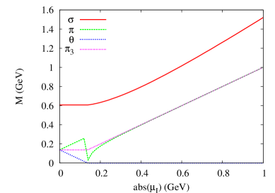
Figure 1: (Color online) Meson masses given by the linear sigma model with the approximation described in the text. Note that $\pi$ and $\theta$ correspond to $\pi_{1}$ and $\pi_{2}$, respectively, at $|\mu_{\mathrm{I}}|<m_{\pi}$.

Figure 2 shows the results at $|\mu_{\mathrm{I}}|=$ 0.5 GeV $\gg m_{\pi}$. Figure 2 (a) is the quasiparticle energy diagram as a function of the relative momentum $k$ (dispersion relation). Its unperturbed structure is quite simple: The positive and negative energy $u$ ($d$) quark levels with $\pm E_{k}$ are shifted upward (downward) by $|\mu_{\mathrm{I}}|/2$. Then, the negative energy $u$, that is the hole state of the $\bar{u}$, and the positive energy $d$ interact around the Fermi surface. This means the $d\bar{u}$ pairing. Hereafter we name these quasiparticle (hole) levels the first, second, third and fourth, from the bottom. The third level, the lower quasiparticle, is the main interest in the following discussion. This lower quasiparticle consists only of $A$ and $C$. In the usual pairing problem, for example in the case of Ref. M. Matsuzaki (1998), this type of $2\times 2$ equation can be cast into the form of the gap equation. In the present case, however, $\pi(k)$ is represented as a function of $A(k^{\prime})$ and $C(k^{\prime})$ as

$$\pi(k)=-\frac{1}{2}\sum_{k^{\prime}}^{\Lambda}(v(k,k^{\prime})2A(k^{\prime})C(k^{\prime})+v^{\prime}(k,k^{\prime})(A^{2}(k^{\prime})-C^{2}(k^{\prime}))),$$

$$2A(k^{\prime})C(k^{\prime})=\frac{\pi(k^{\prime})}{e(k^{\prime})-\frac{m_{1}(k^{\prime})+\tilde{m}_{2}(k^{\prime})}{2}},$$

$$A^{2}(k^{\prime})-C^{2}(k^{\prime})=\frac{E_{k^{\prime}}+\frac{\mu_{\mathrm{I}}}{2}+\frac{m_{1}(k^{\prime})-\tilde{m}_{2}(k^{\prime})}{2}}{e(k^{\prime})-\frac{m_{1}(k^{\prime})+\tilde{m}_{2}(k^{\prime})}{2}}.$$ (29)

Therefore the $v^{\prime}$ term due to the $\sigma$–$\pi$ mixing prevents one from casting Eq.(22) into the form of the gap equation. Nevertheless, the notion of the pair wave function F. Pistolesi and G. C. Strinati (1994) is useful for looking into the physical contents since $A^{2}-C^{2}$ is small around the Fermi surface. Figure 2 (b) shows the Bogoliubov amplitudes $A$ and $C$. Aside from the bump around $k=0$ mentioned below, the hole character changes gradually to the particle character around the Fermi surface as the usual Cooper pairing. This leads to the peak in the pair wave function $\phi(k)=A(k)C(k)$ (see Eq.(29)) shown in Fig. 2 (c). The bump around $k=0$ is a novel feature of the present case; this is brought about by the mesonic contribution $\langle\pi\rangle$ to the gap function $\pi(k)$ (see Eq.(25)) as shown in Fig. 2 (d). In this gap function, the mesonic and the Cooper pair components are comparable around the Fermi surface, whereas the former is dominant around $k=0$ because of the $k$ dependence $\propto M_{q}/E_{k}$.

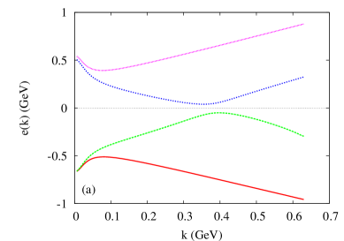
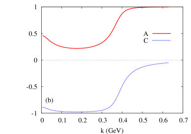
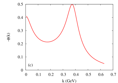
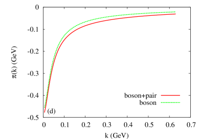
Figure 2: (Color online) Momentum dependence of various quantities at $\mu_{\mathrm{I}}=-0.5$ GeV: (a) the quasiparticle energies, (b) the Bogoliubov amplitudes, (c) the pair wave function, and (d) the gap function. Note that (b) – (d) are associated with the third (from the bottom) solution in (a).

Figure 3 shows the $\mu_{\mathrm{I}}$ dependence of various quantities. Figure 3 (a) shows the pair wave functions at several $\mu_{\mathrm{I}}$s as functions of the momentum. This shows that, leaving room for possible error related to the discussion about Fig. 1, at low $|\mu_{\mathrm{I}}|$ the peak due to the Cooper pairing can not be seen. Actually, $q$ and $\bar{q}$ are bound to each other for $|\mu_{\mathrm{I}}|<2M_{q}$ as shown in Fig. 3 (b). Thus, we can conclude that the pionic condensation has a mixed character: Purely bosonic just after the appearance of the condensation, then the Cooper pairing gradually grows as $|\mu_{\mathrm{I}}|$ increases with retaining significant bosonic component. To look into the spatial structure of Cooper pairs more closely, we Fourier transform $\phi(k)$ as

$$\phi(r)=\frac{1}{2\pi^{2}}\int_{0}^{\Lambda}\phi(k)j_{0}(kr)k^{2}dk.$$ (30)

The results for several $\mu_{\mathrm{I}}$s are shown in Fig. 3 (c) as functions of the relative distance. Obviously those for higher $|\mu_{\mathrm{I}}|$ wave till longer distance. Figure 3 (d) graphs the coherence length,

$$\xi=\left(\frac{\int_{0}^{\Lambda}|\frac{d\phi}{dk}|^{2}k^{2}dk}{\int_{0}^{\Lambda}|\phi|^{2}k^{2}dk}\right)^{1/2},$$ (31)

and 3 (e) the gap at the Fermi surface as functions of $\mu_{\mathrm{I}}$. The obtained coherence length at low $|\mu_{\mathrm{I}}|$ is consistent with the value obtained by an analysis of the $\pi$-$\pi$ scattering, $\langle r^{2}\rangle_{S}^{\pi}=0.61\pm 0.04$ fm² G. Colangelo et al. (2001). In relation to heavy ion collisions, this value is very close to the typical inter-pion distance $d$ at the freeze-out: An example of numbers, the charged particle multiplicity $N_{\mathrm{c}}=555$ B. B. Back et al. (2000) and the source size $V=(\mathrm{6.48fm})^{3}$ W. Broniowski and W. Florkowski (2001), and the fact that the pion is the most abundant, lead to $d\gtrsim(V/N_{\mathrm{c}})^{1/3}=$ 0.79 fm. The picture of a gas of bound mesons may apply to $\xi<d$ while that of a liquid (see also Ref. A. Ayala and A. Smerzi (1997)) of Cooper pairs would be appropriate for $\xi>d$ although the latter realizes at rather high $|\mu_{\mathrm{I}}|$. Figure 3 clearly indicates that the Cooper pairing becomes weakly coupled as $|\mu_{\mathrm{I}}|$ increases. Comparing these figures with corresponding ones in Ref. M. Matsuzaki (2000), one can see that the Cooper pairing part of the present case is more weakly coupled than the case of color superconductivity, as represented by the narrower peak in $\phi(k)$ and longer spatial extent. Figure 3 (d) also shows the cutoff dependence; the dependence is weak.

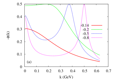
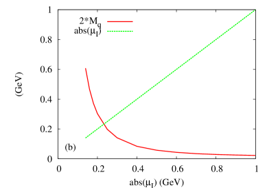
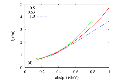
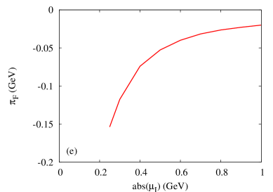
Figure 3: (Color online) Isospin chemical potential dependence of various quantities: (a) the $k$ space pair wave function, (b) the twice of the constituent quark mass, (c) the $r$ space pair wave function, (d) the coherence length, and (e) the gap at the Fermi surface. (d) also contains the cutoff dependence.

At higher $|\mu_{\mathrm{I}}|$, in the present calculation $|\mu_{\mathrm{I}}|\geq$ 0.8 GeV, a gapless pairing ($e<0$) takes place. The gapless dispersion is known to occur in the case of pairing between particles with different masses S.-T. Wu and S. Yip (2003). In the present case, the Fock term produces the difference in the mass (see the denominator in Eq.(29)).

Finally we look into the character of the fourth level, the higher quasiparticle, that corresponds to the Dirac sea pairing in Ref. M. Matsuzaki (1998). This level is of almost pure $u$ quark particle character ($D(k)\simeq 1$) for $k\gtrsim$ 0.1 GeV; but the $\bar{d}$ component strongly mixes around $k=0$ because of two reasons: 1) $\langle\pi\rangle$ equally contributes to $\tilde{\pi}(k)$ and $\pi(k)$ (but with the opposite sign), and 2) the unperturbed energy difference between $u$ and $\bar{d}$ is the same as that between $\bar{u}$ and $d$ at $k=0$.

To summarize, we have studied the momentum dependence of the pionic gap function $\pi(k)$ that determines the spatial structure of the condensation by adopting the linear sigma model as an inter-quark interaction at finite isospin chemical potential as a first step towards the study of the asymmetric matter in the real world. Although confinement is not taken into account in the present study, the character of the condensation is bosonic at low $|\mu_{\mathrm{I}}|$, then the Cooper pairing gradually grows as $|\mu_{\mathrm{I}}|$ increases. This $q$–$\bar{q}$ pairing is weaker than the $q$–$q$ pairing of the case of color superconductivity. The spatial structure (wave function) of the composite pionic system is expected to be measured in lattice QCD simulations as well as the $\mu_{\mathrm{I}}$ dependence of the magnitude of the condensation as signatures of the BEC–BCS crossover. The spatial structure may affect the description of pions created in heavy ion collisions.

Appendix A The Gor’kov formalism

Gor’kov L. P. Gor’kov (1958) first proposed a field theoretical method to describe the pairing problem. In addition to the normal Green function $G(x-x^{\prime})$, the anomalous Green function $F^{\dagger}(x-x^{\prime})$ of $\langle T(\psi^{\dagger}\psi^{\dagger})\rangle$ type is introduced there. The equation of motion of their Fourier transforms is given by

$$\left(\begin{array}[]{@{\,}cc@{\,}}\omega-\xi_{k}&-i\Delta\\ i\Delta&\omega+\xi_{k}\end{array}\right)\left(\begin{array}[]{@{\,}c@{\,}}G(\omega,\mathbf{k})\\ F^{\dagger}(\omega,\mathbf{k})\end{array}\right)=\left(\begin{array}[]{@{\,}c@{\,}}1\\ 0\end{array}\right),$$ (32)

where $\xi_{k}$ and $\Delta$ are the single particle energy measured from the Fermi surface and the momentum independent pairing gap, respectively. Its solution is

$$G(\omega,\mathbf{k})=\frac{u_{k}^{2}}{\omega-\mathcal{E}_{k}}+\frac{v_{k}^{2}}{\omega+\mathcal{E}_{k}},$$

$$F^{\dagger}(\omega,\mathbf{k})=\frac{-i\Delta/2\mathcal{E}_{k}}{\omega-\mathcal{E}_{k}}+\frac{i\Delta/2\mathcal{E}_{k}}{\omega+\mathcal{E}_{k}},$$

$$u_{k}^{2}=\frac{1}{2}\Big{(}1+\frac{\xi_{k}}{\mathcal{E}_{k}}\Big{)},\quad v_{k}^{2}=\frac{1}{2}\Big{(}1-\frac{\xi_{k}}{\mathcal{E}_{k}}\Big{)},$$

$$u_{k}^{2}v_{k}^{2}=\Big{(}\frac{\Delta}{2\mathcal{E}_{k}}\Big{)}^{2},\quad\mathcal{E}_{k}=\sqrt{\xi_{k}^{2}+\Delta^{2}}.$$ (33)

Substituting them back to Eq.(32) gives

$$\left(\begin{array}[]{@{\,}cc@{\,}}\frac{[(\omega-\xi_{k})u_{k}-\Delta v_{k}]u_{k}}{\omega-\mathcal{E}_{k}}+\frac{[(\omega-\xi_{k})v_{k}+\Delta u_{k}]v_{k}}{\omega+\mathcal{E}_{k}}\\ i\frac{[\Delta u_{k}-(\omega+\xi_{k})v_{k}]u_{k}}{\omega-\mathcal{E}_{k}}+i\frac{[\Delta v_{k}+(\omega+\xi_{k})u_{k}]v_{k}}{\omega+\mathcal{E}_{k}}\end{array}\right)=\left(\begin{array}[]{@{\,}c@{\,}}1\\ 0\end{array}\right).$$ (34)

The residues at $\omega=\mathcal{E}_{k}$ (quasiparticle) lead to

$$\left(\begin{array}[]{@{\,}cc@{\,}}\xi_{k}&\Delta\\ \Delta&-\xi_{k}\end{array}\right)\left(\begin{array}[]{@{\,}c@{\,}}u_{k}\\ v_{k}\end{array}\right)=\mathcal{E}_{k}\left(\begin{array}[]{@{\,}c@{\,}}u_{k}\\ v_{k}\end{array}\right).$$ (35)

Those at $\omega=-\mathcal{E}_{k}$ (quasihole) lead to the same equation. Therefore the equation for the Green functions and that for the Bogoliubov amplitudes are equivalent.

Appendix B The Bogoliubov transformation

Replacing the spin $\sigma=\uparrow/\downarrow$ and $a_{-\mathbf{k}}$ in the non-relativistic pairing problem by the isospin $u/d$ and $b_{-\mathbf{k}}$, respectively, we obtain two Bogoliubov transformations relevant to the present case,

$$\begin{split}&\left(\begin{array}[]{@{\,}c@{\,}}a_{u}\\ b_{-d}^{\dagger}\end{array}\right)=\left(\begin{array}[]{@{\,}cc@{\,}}u^{1}&-v^{2}\\ v^{2}&-u^{1}\end{array}\right)\left(\begin{array}[]{@{\,}c@{\,}}\eta_{u}\\ \eta_{-d}^{\dagger}\end{array}\right),\\ &\left(\begin{array}[]{@{\,}c@{\,}}a_{d}\\ b_{-u}^{\dagger}\end{array}\right)=\left(\begin{array}[]{@{\,}cc@{\,}}u^{2}&v^{1}\\ v^{1}&u^{2}\end{array}\right)\left(\begin{array}[]{@{\,}c@{\,}}\eta_{d}\\ \eta_{-u}^{\dagger}\end{array}\right),\end{split}$$ (36)

at each momentum and spin.

Since there is $i\gamma^{5}\overrightarrow{\tau}$ between two flavors, here we take $u^{1}$ and $v^{1}$ are imaginary, $u^{2}$ and $v^{2}$ are real. Then the two types of quasiparticle, $\eta_{u}^{\dagger}$ and $\eta_{d}^{\dagger}$, can be represented collectively as

$$\eta^{\dagger}=\sum_{i=1}^{2}(u^{i}a_{i}^{\dagger}+v^{i}b_{-i}),$$ (37)

where $i=1/2$ correspond to $u/d$.