Dynamic polarization of graphene by moving external charges: random phase approximation

Abstract

We evaluate the stopping and image forces on a charged particle moving parallel to a doped sheet of graphene by using the dielectric response formalism for graphene’s $\pi$-electron bands in the random phase approximation (RPA). The forces are presented as functions of the particle speed and the particle distance for a broad range of charge-carrier densities in graphene. A detailed comparison with the results from a kinetic equation model reveal the importance of inter-band single-particle excitations in the RPA model for high particle speeds. We also consider the effects of a finite gap between graphene and a supporting substrate, as well as the effects of a finite damping rate that is included through the use of Mermin’s procedure. The damping rate is estimated from a tentative comparison of the Mermin loss function with a HREELS experiment. In the limit of low particle speeds, several analytical results are obtained for the friction coefficient that show an intricate relationship between the charge-carrier density, the damping rate, and the particle distance, which may be relevant to surface processes and electrochemistry involving graphene.

I Introduction

The interactions of fast-moving charged particles with various carbon nanostructures have been studied extensively in the context of electron energy loss spectroscopy (EELS), typically using a scanning transmission electron microscope (STEM) with incident electron energies on the order of 100 keV. This technique has proven to be a powerful tool for investigating the dynamic response of carbon nanotubes Stephan_2002 ; Kramberger_2008 and, more recently, graphene.Eberlein_2008 At such high incident electron energies, these studies have revealed important properties of both high-frequency $\sigma+\pi$ plasmon excitations ($\sim 15-30$ eV) and low-frequency $\pi$ plasmon excitations ($\sim 5$ eV) in isolated single-wall carbon nanotubes Kramberger_2008 and in free-standing, undoped graphene.Eberlein_2008 While the studies on carbon nanotubes typically give plasmon dispersions at large wavenumbers ($>0.1$ Å^-1) in the axial direction, Stephan_2002 ; Kramberger_2008 the study on graphene was performed with an electron momentum transfer close to zero, although it integrated over a significant in-plane component of the plasmon wave vector.Eberlein_2008 In both cases, experimental data was found to be in good agreement with ab initio calculations.Kramberger_2008 ; Eberlein_2008 ; Trevisanutto_2008 In addition to ab initio calculations, methods employing an empirical dielectric tensor Taverna_2002 and a two-fluid, two-dimensional (2D) hydrodynamic model for graphene Mowbray_2006 ; Radovic_2007 have also been able to reproduce the basic features of the $\sigma+\pi$ and $\pi$ plasmon excitations in carbon nanostructures.

For lower-energy external moving charges, recent progress has been made in measuring the dispersion of low-frequency plasmon excitations on solid surfaces using high-resolution reflection EELS (HREELS) with incident electron energies on the order of 10 eV. Such a measurement was performed on metallic surface-state electron bands, Diaconescu_2007 and the results were interpreted theoretically using a dielectric-response model within the random phase approximation (RPA) that took into account the typically parabolic band structures of the surface states. Diaconescu_2007 ; Alducin_2007 ; Silkin_2008 Furthermore, Liu et al. Liu_2008 have used HREELS to compare the low-frequency excitation spectra of doped graphene on a SiC substrate with the spectra of a metallic monolayer on a semiconducting Si substrate. At such low incident electron energies, the authors were able to measure the $\pi$ plasmon dispersion in a range of small wavenumbers ($<0.2$ Å^-1) for a doped sheet of graphene with a high charge-carrier density. Liu_2008 This HREELS experiment, which provides the wavenumber-resolved spectra of low-frequency excitation modes in graphene with a high sensitivity to the doping level, Liu_2008 is more relevant to the parameter space in the present work than the STEM-EELS experiments.

It is well appreciated that doping plays an immensely important role in graphene’s conducting properties, for which electron scattering on statically-screened charged impurities situated near graphene is one of the most important processes and is likely responsible for the famed minimum conductivity in undoped graphene. Novoselov_2005 ; Ando_2006 ; Peres_2007 ; Sarma_2007 ; PNAS_2007 ; Adam_2008 ; Chen_2008 ; Castro_2009 In this context, important progress has been made in the development and use of the RPA dielectric function for low-energy excitations involving graphene’s $\pi$ electron bands in the approximation of linearized electron energy dispersion, which gives rise to the picture of massless Dirac fermions (MDF). Shung_1986 ; Wunsch_2006 ; Hwang_2007 ; Barlas_2007 This progress has opened up a range of interesting problems involving the interaction of graphene with external charges moving sufficiently slow that the MDF-RPA dielectric response theory can be applied. While an obvious application of this theory would be to interpret the HREELS experiment Liu_2008 on graphene, another interesting application would be to the study of slow, heavy particles moving near graphene. This latter application of graphene’s MDF-RPA dielectric response theory would be relevant to studies of chemisorption of alkali-metal atoms, Khantha_2004 friction of migrating atoms and molecules Tomassone_1997 ; Dedkov_2005 moving near graphene, and ion transport in aqueous solutions adjacent to graphene when top-gating with an electrolyte is implemented. Bazant_2004 Moreover, one could explore the application of low-energy, ion-surface scattering techniques Brongersma_2007 to graphene and other carbon nanostructures. There has also been recent interest in the directional effects of ion interactions with graphene-based materials, such as low-energy ion channeling through carbon nanotubes Miskovic_2007 and ion interactions with highly-oriented pyrolytic graphite, including implantation, Ramos_2001 channeling, Yagi_2004 and ion-induced secondary electron emission from this target. Cernusca_2005 If applied to graphene, most of the scattering configurations in these studies would involve impacts of slow, heavy particles under grazing angles of incidence, and many interesting parallels may be found with Winter’s experiments on the grazing scattering of ions and atoms from solid surfaces. Winter_2002

We therefore wish to study the application of the MDF-RPA model to charged particles moving parallel to a single layer of supported graphene under gating conditions. In the wavenumber-frequency domain, $(q,\omega)$, the MDF-RPA model is applicable to graphene’s polarization modes if the conditions $q<2k_{c}$ and $\omega<2\varepsilon_{c}/\hbar$ are satisfied, where $k_{c}\approx a^{-1}$ is a high-momentum cut-off (with lattice constant $a\approx$ 2.46 Å) and $\varepsilon_{c}\approx$ 1 eV is a high-frequency cut-off validating the approximation of linearized $\pi$ electron bands. Wunsch_2006 ; Barlas_2007 ; Castro_2009 For a point charge moving parallel to graphene at a fixed distance $z_{0}$ and constant speed $v$, the former condition will be satisfied only for distances $z_{0}>a$, and hence we may neglect both the size of the particle and the size of the $\pi$ electron orbitals in graphene. The latter condition can be transformed into a restriction on the particle speed by invoking the Bohr’s adiabatic criterion and requiring that $v/z_{0}<2\varepsilon_{c}/\hbar$. It is clear that with a gap on the order of 7 eV for graphene’s $\sigma$ bands, particles moving at such slow speeds and large distances cannot excite the high-energy modes involving graphene’s $\sigma$ electrons.

Within the constraints of the MDF-RPA model, the main focus of this paper is on the stopping force and the dynamic image force acting on an external charged particle. We note that the stopping force is equal to the negative of the stopping power, which is defined as the energy loss of the external particle per unit length along its trajectory. Winter_2002 Meanwhile, the image force is a conservative force Gumbs_2009 that can strongly deflect a particle’s trajectory, especially for low particle speeds and/or small angles of incidence upon the target’s surface. Winter_2002 This was demonstrated not just for electron interactions with solid surfaces, Echenique_1985 ; Lambin_1987 ; Inaoka_2001 but also for ion Song_2003 and molecule Song_2005 grazing scattering from solid surfaces and ion Zhou_2005 ; Borka_2006 and molecule Zhou_2006 ; Mowbray_2007 channeling through carbon nanotubes. For example, in Ref.Song_2003 it was shown that both the stopping and image forces must be treated in a self-consistent manner in order to model ion trajectories and obtain ion energy losses that agree well with experiment results for the grazing scattering of slow, highly-charged ions on various surfaces. Fritz_1996 ; Juaristi_1999 A discussion of the stopping and image forces in the MDF-RPA model is therefore relevant to the current literature.

In our previous work, Radovic_2008 we have calculated the stopping and image forces on charged particles moving above graphene by assuming a high equilibrium density, $n$, of charge carriers in graphene and using a kinetic (Vlasov) equation to describe the response of graphene’s $\pi$ bands within the linearized electron energy dispersion approximation. Radovic_2008 ; Ryzhii_2007 This semi-classical kinetic equation (SCKE) model gave a relatively simple dielectric function for graphene that accurately described the thermal effect on plasmon dispersion Ryzhii_2007 ; Vafek_2006 and allowed us to analyze the contributions of plasmon excitations and low-energy intra-band single-particle excitations (SPEs) to the stopping and image forces. Radovic_2008 However, it remained unclear how large the density must be to validate the semi-classical model and, more importantly, what effect the inter-band SPEs that lie beyond the capability of the SCKE model have. Therefore, the first goal of this paper is to determine the conditions under which the SCKE model is applicable at zero temperature by comparing the stopping and image forces obtained using the SCKE dielectric function Radovic_2008 with those obtained using the MDF-RPA dielectric function. Wunsch_2006 ; Hwang_2007 ; Barlas_2007 Furthermore, since we have found in Ref. Radovic_2008 that a finite gap between graphene and the substrate strongly affects both forces in the SCKE model, the second goal of this paper is to examine the effect of a finite gap in the MDF-RPA model. We note that the issue of a finite gap has become more important as increasingly diverse dielectric environments for graphene are studied. Jang_2008

Although we consider the MDF-RPA dielectric function to be a basic, parameter-free model that provides an adequate description of the inter-band SPEs in graphene, the model nevertheless has its shortcomings. For example, it ignores the local-field effects (LFE) due to electron-electron correlations Trevisanutto_2008 ; Kramberger_2008 and assigns an infinitely long lifetime to the electron excitations. The latter deficiency is often rectified in ab initio studies by applying a finite broadening, on the order of 0.5 eV, to the frequency domain for calculations of the loss function. Eberlein_2008 In a similar way, one can introduce a finite relaxation time, or decay (damping) rate, $\gamma$, to the MDF-RPA dielectric function for graphene using Mermin’s procedure. Mermin_1970 ; Qaiumzadeh_2008 Since there are many scattering processes that can give rise to a finite lifetime of the excited $\pi$ electrons in graphene, an accurate determination of $\gamma$ still presents a challenge.Hwang_2008 ; Qaiumzadeh_2008 Therefore, the third goal of this paper is to treat $\gamma$ as an empirical parameter and investigate the effects of a finite damping rate on the stopping and image forces calculated with a MDF-RPA dielectric function modified by the Mermin procedure. This dielectric function, hereafter referred to as the Mermin dielectric function, requires a careful extension of the MDF-RPA dielectric function derived for $\gamma=0$ in Refs.Wunsch_2006 ; Hwang_2007 to finite $\gamma$. Details of the Mermin dielectric function are given in Appendix A.

The parameters of primary interest in this study are therefore the equilibrium density of charge carriers in graphene, $n$, the graphene-substrate gap height, $h$, and the damping rate, $\gamma$. The equilibrium density is particularly important because it determines the Fermi momentum of graphene’s $\pi$-electron band, $k_{F}=\sqrt{\pi n}$, and the corresponding Fermi energy, $\varepsilon_{F}=\hbar v_{F}k_{F}$, where $v_{F}\approx c/300$ is the Fermi speed of the linearized $\pi$ band and $c$ is the speed of light in free space. In the case of intrinsic graphene ($n=0$), the Fermi energy coincides with the Dirac point, $\varepsilon_{F}=0$. In this paper, we consider a wide range of densities $n\geq 0$, expressed as a multiple of the base value $n_{0}=10^{11}$ cm^-2, under the conditions $k_{F}<k_{c}$ and $\varepsilon_{F}<\varepsilon_{c}$.

The rest of the paper is outlined as follows. In section II, we present a theoretical derivation of the interaction of a general charge distribution with a layer of supported graphene. This derivation motivates the definition of the stopping and image forces for a point charge. In section III, we compare the stopping and image forces in the MDF-RPA and SCKE models for the simple case of free graphene and a vanishing damping rate to determine the range of densities for which the SCKE model is valid. We then focus on the MDF-RPA model with a vanishing damping rate, and in section IV we investigate the effects of a finite gap between graphene and a SiO₂ substrate. In the simplified case of a zero gap, we provide analytic expressions for the stopping and image forces for intrinsic graphene and low particle speeds. Finally, in section V we consider the MDF-RPA model with a finite damping rate. After comparing the MDF-RPA model with experimental data to estimate the value of the damping rate, we consider the effects of the damping rate on the stopping and image forces with a special focus on the stopping force at low particle speeds. Note that we use Gaussian electrostatic units.

II Basic theory

We first give a brief generalization of the formalism developed in Ref.Radovic_2008 to the case of a charge distribution with density $\rho_{\mathrm{ext}}({\bf r},z,t)$. We assume that the charge distribution moves along a classical trajectory in a Cartesian system with graphene placed in the $z=0$ plane and with coordinates ${\bf r}=\{x,y\}$ in the graphene plane. In keeping with the reflection geometry of ion-surface grazing scattering, Winter_2002 we assume that the external charge distribution remains localized in the region $z>0$ above graphene while a semi-infinite substrate occupies the region $z<-h$ below graphene. Following Ref.Radovic_2008 , we can express the induced potential $\Phi_{\mathrm{ind}}({\bf r},z,t)$ in the region above graphene using the Fourier transform (${\bf r}\rightarrow{\bf q}$ and $t\rightarrow\omega$) as

$$\widetilde{\Phi}_{\mathrm{ind}}^{>}({{\bf q}},z,\omega)=\left[\frac{1}{\epsilon({\bf q},\omega)}-1\right]\widetilde{\Phi}_{\mathrm{ext}}^{0}({{\bf q}},\omega)\,\mathrm{e}^{-qz},$$ (1)

where $\epsilon({\bf q},\omega)$ is the dielectric function of the combined graphene-substrate system and $\widetilde{\Phi}_{\mathrm{ext}}^{0}({\bf q},\omega)$ is the Fourier transform of the external potential evaluated at the graphene plane, $z=0$. The dielectric function of the system can be written as

$$\epsilon({\bf q},\omega)=\epsilon_{\text{bg}}(q)+\frac{2\pi e^{2}}{q}\Pi({\bf q},\omega),$$ (2)

where $\Pi({\bf q},\omega)$ is the polarization function for free graphene and $\epsilon_{\text{bg}}(q)$ is the effective background dielectric function, which is expressed in terms of the substrate dielectric constant $\epsilon_{\text{sub}}$ as Radovic_2008

$$\epsilon_{\text{bg}}(q)=\frac{\epsilon_{\text{sub}}+1}{2}\,\frac{1+\coth(qh)}{\epsilon_{\text{sub}}+\coth(qh)}.$$ (3)

We note that, instead of dielectric constant $\epsilon_{\text{sub}}$, one may use a frequency dependent substrate bulk dielectric function, $\epsilon_{\text{sub}}(\omega)$, in order to include the effects of coupling between graphene’s $\pi$ electrons and either the surface phonon modes in a strongly polar insulating substrate or the surface plasmon modes in a metallic substrate under the local approximation. Fischetti_2001 In the former case, which includes a substrate with a single transverse optical (TO) phonon mode at frequency $\omega_{\mathrm{TO}}$, one may use a dielectric function of the form Fratini_2008

$$\epsilon_{\text{sub}}(\omega)=\epsilon_{\infty}+\left(\epsilon_{s}-\epsilon_{\infty}\right)\frac{\omega_{\mathrm{TO}}^{2}}{\omega_{\mathrm{TO}}^{2}-\omega\!\left(\omega+i\gamma_{\mathrm{TO}}\right)},$$ (4)

where $\epsilon_{s}=\epsilon_{\text{sub}}(0)$ and $\epsilon_{\infty}=\lim_{\omega\rightarrow\infty}\epsilon_{\text{sub}}(\omega)$ are the static and high-frequency dielectric constants of the substrate, respectively. In the latter case, which includes the high-frequency response of a metal, one may use the Drude dielectric function $\epsilon_{\text{sub}}(\omega)=1-\omega_{p}^{2}/\!\left[\,\omega\!\left(\omega+i\gamma_{p}\right)\right]$ with a plasma frequency $\omega_{p}$ and a damping rate $\gamma_{p}$.

We limit the focus of this work to an insulating substrate in the static mode with a dielectric constant $\epsilon_{\text{sub}}=\epsilon_{s}$, but we allow for an arbitrary gap $h$ between graphene and the substrate. We note, however, that it is common in the literature to assume a zero gap, Wunsch_2006 ; Hwang_2007 ; PNAS_2007 ; Adam_2008 for which Eq. (3) gives an effective background dielectric constant $\epsilon_{\text{bg}}^{0}=(\epsilon_{\text{s}}+1)/2$. In this case, a simple description of the screening of electron-electron interactions in graphene can be quantified by the Wigner-Seitz radius, $r_{s}=e^{2}/(\epsilon_{\text{bg}}^{0}\hbar v_{F})$, Hwang_2007 and free graphene can be recovered by setting $\epsilon_{\text{s}}=1$, and hence $\epsilon_{\text{bg}}^{0}=1$. Results provided for $h=0$ are therefore slightly more general than results provided for $h\rightarrow\infty$, which also characterizes free graphene by yielding $\epsilon_{\text{bg}}=1$ in Eq. (3).

Next, we write $\widetilde{\Phi}_{\mathrm{ext}}^{0}({\bf q},\omega)=\frac{2\pi}{q}S({\bf q},\omega)$, where the external charge structure factor $S({\bf q},\omega)$ is given by

$$S({\bf q},\omega)=\int\limits_{-\infty}^{\infty}dt\,\mathrm{e}^{i\omega t}\int d^{2}{\bf r}\,\mathrm{e}^{-i{\bf q}\cdot{\bf r}}\int\limits_{0}^{\infty}dz\,\mathrm{e}^{-qz}\,\rho_{\mathrm{ext}}({\bf r},z,t).$$ (5)

For a point charge $Ze$ moving parallel to graphene with velocity ${\bf v}$ and at a fixed distance $z_{0}>0$, we find that $S({\bf q},\omega)=2\pi Ze\,\delta(\omega-{\bf q}\cdot{\bf v})\,\mathrm{e}^{-qz_{0}}$. In this case, the induced electric field ${\bf E}^{>}_{\mathrm{ind}}({\bf r},z,t)=-\nabla\Phi_{\mathrm{ind}}^{>}({\bf r},z,t)$ can be written as

$${\bf E}^{>}_{\mathrm{ind}}({\bf r},z,t)=\frac{Ze}{2\pi}\times$$

$$\int d^{2}{\bf q}\,\left(\,{\bf\hat{z}}-i{\bf\hat{q}}\right)\,\mathrm{e}^{i{\bf q}\cdot({\bf r}-{\bf v}t)}\,\mathrm{e}^{-q\left(z+z_{0}\right)}\,\left[\frac{1}{\epsilon({\bf q},{\bf q}\cdot{\bf v})}-1\right],$$ (6)

where ${\bf\hat{z}}$ is a unit vector perpendicular to graphene and ${\bf\hat{q}}={\bf q}/q$. For stopping and image forces defined by $F_{s}=Ze\,{\bf\hat{v}}\cdot{\bf E}^{>}_{\mathrm{ind}}({\bf r}\!=\!{\bf v}t,z\!=\!z_{0},t)$ and $F_{i}=Ze\,{\bf\hat{z}}\cdot{\bf E}^{>}_{\mathrm{ind}}({\bf r}\!=\!{\bf v}t,z\!=\!z_{0},t)$, respectively, where ${\bf\hat{v}}={\bf v}/v$, one obtains Radovic_2008

$$F_{\text{s}}=\frac{2}{\pi}\frac{Z^{2}e^{2}}{v}\times$$

$$\int_{0}^{\infty}dq\,\mathrm{e}^{-2qz_{0}}\int_{0}^{qv}d\omega\,\frac{\omega}{\sqrt{q^{2}v^{2}-\omega^{2}}}\,\,\Im\!\left[\frac{1}{\epsilon(q,\omega)}\right],$$ (7)

$$F_{\text{i}}=\frac{2}{\pi}Z^{2}e^{2}\times$$

$$\int_{0}^{\infty}dq\,q\,\mathrm{e}^{-2qz_{0}}\int_{0}^{qv}\frac{d\omega}{\sqrt{q^{2}v^{2}-\omega^{2}}}\,\,\Re\!\left[\frac{1}{\epsilon(q,\omega)}-1\right].$$ (8)

Note that we have used the symmetry properties of the MDF-RPA dielectric function $\epsilon(q,\omega)$ to simplify Eqs. (7) and (8).

For the comparison with the HREELS experiment Liu_2008 in section V, we also define the total energy of the external charge reflected from graphene as

$$E_{\mathrm{loss}} = -\int\limits_{-\infty}^{\infty}dt\int d^{2}{\bf r}\int\limits_{-\infty}^{\infty}dz\,\rho_{\mathrm{ext}}({\bf r},z,t)\,\frac{\partial}{\partial t}\Phi_{\mathrm{ind}}({\bf r},z,t)$$ (9)

$$= \int\limits_{0}^{\infty}d\omega\,\omega\int\frac{d^{2}{\bf q}}{2\pi^{2}}\,|S({\bf q},\omega)|^{2}\,\Im\!\left[\frac{-1}{\epsilon({\bf q},\omega)}\right].$$

For a point charge $Ze$ moving on a specular-reflection trajectory with $\rho_{\mathrm{ext}}({\bf r},z,t)=Ze\,\delta\!\left({\bf r}\!-\!{\bf v}_{\parallel}t\right)\delta\!\left(z\!-\!v_{\perp}|t|\right)$, where ${\bf v}_{\parallel}$ and $v_{\perp}$ are the components of the particle velocity parallel and perpendicular to the graphene plane, respectively, the probability density for exciting the mode with frequency $\omega$ and wavevector ${\bf q}$ is Ibach_1982

$$P({\bf q},\omega)=\frac{2}{\pi^{2}}\frac{(Ze)^{2}v_{\perp}^{2}q}{\left[\left(\omega-{\bf q}\cdot{\bf v}_{\parallel}\right)^{2}+\left(qv_{\perp}\right)^{2}\right]^{2}}\,\Im\!\left[\frac{-1}{\epsilon({\bf q},\omega)}\right],$$ (10)

where we have set the reflection coefficient to unity.

III Comparison with semi-classical model

In this section, we present the stopping and image forces calculated with dielectric functions from the SCKE model Radovic_2008 and the MDF-RPA model Wunsch_2006 ; Hwang_2007 for free graphene ($\epsilon_{\text{bg}}^{0}=1$) and a vanishing damping rate ($\gamma\rightarrow 0$). The results for both forces are normalized by $F_{0}=Z^{2}e^{2}/(4z_{0}^{2})$, the magnitude of the classical image force on a static point charge a distance $z_{0}$ from a perfect conductor, to better reveal differences between the two models.

Before proceeding, we note that the infinite upper limits of the $q$ integrals in Eqs. (7) and (8) cause both forces to diverge as the distance $z_{0}$ goes to zero. This behaviour, which also occurs in models of solid surfaces, Barton_1979 ; Lucas_1979 should not be a major concern because the restriction $z_{0}>a$ is necessary to ensure the validity of the MDF approximation. However, if one would like to extend the results for the stopping and image forces to include small distances, a standard procedure to eliminate the divergence at $z_{0}$ is to adopt a high-momentum cut-off. Barton_1979 ; Lucas_1979 For studies of electronic processes in graphene with no external charges, it is common to impose a sharp cut-off at approximately $k_{c}$. Wunsch_2006 ; Barlas_2007 ; Castro_2009 However, there are other mathematical methods for imposing a cut-off besides this sharp truncation of the $q$ integration. Lucas_1979 As discussed in Ref.Lucas_1979 , the use of an exponential cut-off function $\mathrm{e}^{-q/k_{c}}$ in Eqs. (7) and (8) would simply amount to a shift of the $z_{0}$ coordinate by a distance on the order of the lattice constant, which is sometimes referred to as an effective image plane. Lucas_1979 ; Gumbs_2009 We therefore evaluate the stopping and image forces using Eqs. (7) and (8) with infinite upper limits in the $q$ integrals, and if one would like an estimate of the order of magnitude of these forces at small distances we note that a suitable shift of the $z_{0}$ axis may be chosen. It should also be mentioned that in an RPA model that takes into account the finite size of graphene’s $\pi$ electron orbitals, the divergence of these forces as $z_{0}\rightarrow 0$ can be removed by the resulting structure factor, which provides a physically motivated algebraic cut-off function. Shung_1986 ; Lucas_1979

Figure 1: The stopping force (a) and image force (b) normalized by $F_{0}=Z^{2}e^{2}/(4z_{0}^{2})$ and shown as a function of the reduced speed $v/v_{F}$ of a proton ($Z=1$) moving at a distance $z_{0}$ = 20 Å above free graphene ($h\rightarrow\infty$) for several values of the reduced charge-carrier density $n/n_{0}$, where $n_{0}=10^{11}$ cm^-2. The thick and thin lines represent the results from the MDF-RPA and SCKE models with vanishing damping ($\gamma=0$), respectively.

In Fig. 1, we compare the velocity dependence of the normalized stopping and image forces on a proton ($Z=1$) moving at a distance $z_{0}=20$ Å above free graphene in the MDF-RPA model (thick lines) and in the SCKE model (thin lines) for a broad range of densities. For intrinsic graphene ($n=0$), note that both forces vanish in the SCKE model but they arise from inter-band SPEs in the MDF-RPA model. Furthermore, it can be seen that the results from the SCKE model agree with those from the MDF-RPA model only for high densities, and that this agreement is better for low particle speeds ($v<v_{F}$) than for high particle speeds ($v>v_{F}$). The large difference between the MDF-RPA and SCKE models at high particle speeds is due to the presence of a plasmon line given by $\omega=\omega_{p}(q)$, Vafek_2006 ; Ryzhii_2007 ; Radovic_2008 where $\omega_{p}(q)=v_{F}(q+q_{s})\sqrt{q/(q+2q_{s})}>qv_{F}$ and $q_{s}\equiv 4r_{s}k_{F}$ is the Thomas-Fermi (TF) inverse screening length. Ando_2006 ; Hwang_2007 ; Radovic_2008 Specifically, the energy loss for high particle speeds in the SCKE model is dominated by the undamped plasmon at frequency $\omega_{p}(q)$, while the presence of the inter-band SPE continuum in the MDF-RPA model for $\omega/v_{F}>\text{max}\left(q,2k_{F}-q\right)$ causes a strong Landau damping of the plasmon, Wunsch_2006 ; Hwang_2007 thereby producing much weaker velocity dependencies. However, even for these high particle speeds it appears that the SCKE model may be partially applicable under the condition $z_{0}k_{F}\gg 1$, which requires heavy doping of graphene in order to reduce the significance of the inter-band SPEs.

Figure 2: The stopping force (a) and image force (b) normalized by $F_{0}=Z^{2}e^{2}/(4z_{0}^{2})$ and shown as a function of the distance $z_{0}$ of a proton ($Z=1$) moving at a reduced speed $v/v_{F}=0.5$ above free graphene ($h\rightarrow\infty$) for several values of the reduced charge-carrier density $n/n_{0}$, where $n_{0}=10^{11}$ cm^-2. The thick and thin lines represent the results from the MDF-RPA and SCKE models with vanishing damping ($\gamma=0$), respectively.

The difference between the SCKE and MDF-RPA models at low particle speeds is further analyzed in Fig. 2. Using the same set of densities as in Fig. 1, we compare the reduced stopping and image forces on a proton ($Z=1$) moving at a speed $v=v_{F}/2$ above free graphene as a function of the particle distance, $z_{0}$. At such low speeds, one can see that the agreement between the SCKE and MDF-RPA models is better for the image force than it is for the stopping force. It follows from Fig. 2 that the condition $z_{0}k_{F}>1$ may suffice as a rough criterion for the application of the SCKE model at low speeds ($v<v_{F}$). This condition is far less restrictive than $z_{0}k_{F}\gg 1$, which is required for the application of the SCKE model at high speeds ($v>v_{F}$). We therefore discontinue further analysis of the SCKE model at high speeds, and turn our focus to analyzing various parameters in the MDF-RPA model alone.

IV MDF-RPA with vanishing damping

In this section, we use the MDF-RPA dielectric function with a vanishing damping rate ($\gamma\rightarrow 0$) to evaluate the stopping and image forces. We first investigate the effects of a finite graphene-substrate gap, and then discuss two important cases with a zero gap: intrinsic graphene ($n=0$) and vanishing particle speeds ($v\rightarrow 0$).

IV.1 Effects of a finite gap

Figure 3: The stopping force (a) and image force (b) from the MDF-RPA model with vanishing damping ($\gamma=0$) shown as a function of the reduced speed $v/v_{F}$ of a proton ($Z=1$) moving at a distance $z_{0}$ = 20 Å above graphene on a SiO₂ substrate ($\epsilon_{\text{s}}\approx 3.9$). Results are shown for several values of the gap height $h$ and several values of the reduced charge-carrier density $n/n_{0}$, where $n_{0}=10^{11}$ cm^-2.

We now assume that graphene is supported by a SiO₂ substrate ($\epsilon_{\text{s}}\approx 3.9$) and explore the effects of a variable gap height. It should be noted that the mean gap height between graphene and a SiO₂ substrate has been measured as 4.2 Å, Ishigami_2007 which is comparable to the equilibrium distance of 3.6 Å found in ab inito calculations between graphene and the topmost atomic plane of a SiO₂ substrate. Romero_2008 However, we note that $h$ is defined in Ref.Radovic_2008 as the position of an effective substrate surface plane where boundary conditions on the electrostatic fields are imposed. Thus, while the measured and theoretically obtained values of the graphene-substrate gap serve as a guide for the value of $h$, there is an uncertainty in $h$ on the same order as the shift of the $z$ axis discussed earlier. In this subsection, we consider the gap heights $h\rightarrow\infty$ for free graphene, $h$ = 4 Å for a realistic value, and $h=0$ for the zero gap commonly considered in the literature.

In Fig. 3, we compare the velocity dependence of the stopping and image forces on a proton moving at a distance $z_{0}=20$ Å above graphene for several gap heights and densities. For low particle speeds ($v<v_{F}$), the gap height has a relatively small influence on the stopping and image forces that diminishes as the charge-carrier density increases and effectively screens out the graphene-substrate gap. The density, $n$, is therefore the most important parameter in the low-speed behaviour of both forces. For higher particle speeds, the charge carriers in graphene are not as effective in screening out the graphene-substrate gap, and hence the gap height has a much stronger effect on the stopping and image forces. In particular, Fig. 3 shows that for sufficiently high speeds ($v\gg v_{F}$) an increase in the gap height tends to increase the strength of the stopping force and decrease the strength of the image force, but there is a range of moderate speeds for which this trend is reversed. Also note that for sufficiently high speeds, all MDF-RPA stopping and image forces approach the intrinsic case, $n=0$.

Figure 4: The stopping force (a) and image force (b) from the MDF-RPA model with vanishing damping ($\gamma=0$) shown as a function of the distance $z_{0}$ of a proton ($Z=1$) moving at a reduced speed $v/v_{F}=6$ above graphene on a SiO₂ substrate ($\epsilon_{\text{s}}\approx 3.9$). Results are shown for several values of the gap height $h$ and several values of the reduced charge-carrier density $n/n_{0}$, where $n_{0}=10^{11}$ cm^-2.

The effect of the gap height at high speeds is further explored in Fig. 4, which shows the distance dependence of the stopping and image forces on a proton moving at a moderately high speed $v=6v_{F}$ above graphene for the same gap heights and densities as in Fig. 3. In Fig. 4, it can be seen that the gap height has a strong influence on both forces for all distances. One may conclude that in the MDF-RPA model, as in the SCKE model, Radovic_2008 any uncertainty or local variations in the gap height across graphene can lead to large fluctuations in the stopping and image forces, particularly for high particle speeds.

IV.2 Intrinsic graphene with a zero gap

We now take advantage of the simplicity of the MDF-RPA dielectric function for intrinsic graphene with a vanishing damping rate Wunsch_2006 ; Hwang_2007 to evaluate the stopping and image forces analytically for a zero gap. In this case, it is worth noting that the distance dependence of both forces can be factored out as $F_{0}=Z^{2}e^{2}/(4z_{0}^{2})$. For the stopping force, we find

$$F_{\text{s}}^{0}=-\frac{F_{0}}{\epsilon_{\text{bg}}^{0}}\,\frac{\rho_{s}}{\nu}\left[1-\left(1+\frac{\nu^{2}-1}{\rho_{s}^{2}}\right)^{-1/2}\right],$$ (11)

where $\rho_{s}\equiv\pi r_{s}/2$ and $\nu\equiv v/v_{F}$. As seen from the thick solid curve in Fig. 1(a), this expression is subject to the velocity threshold constraint $v>v_{F}$, which is a consequence of the inter-band SPEs yielding the loss function $-\Im\epsilon(q,\omega)>0$ only for $\omega>qv_{F}$. Wunsch_2006 ; Hwang_2007 For sufficiently high particle speeds ($v\gg v_{F}$), one obtains an asymptotic form $F_{\text{s}}^{0}\sim-(\pi/8)\,\left[Ze^{2}/(\epsilon_{\text{bg}}^{0}z_{0})\right]^{2}/\left(\hbar v\right)$ that is independent of $v_{F}$. It is interesting to note that the MDF-RPA stopping forces for all densities approach this high-speed asymptotic limit, as seen in Fig. 1(a) for free graphene and in Fig. 3(a) for various gap heights.

The corresponding expression for the image force on a charged particle moving above intrinsic graphene, $F_{\text{i}}^{0}$, is rather cumbersome. We therefore define the effective background dielectric constant $\epsilon_{\text{bg}}^{*}$ by writing the image force in the form $F_{\text{i}}^{0}=F_{0}\left(1/\epsilon_{\text{bg}}^{*}-1\right)$, and in Fig. 5 we present $\epsilon_{\text{bg}}^{*}$ as a function of the particle speed $v$ and the actual background dielectric constant $\epsilon_{\text{bg}}^{0}=(\epsilon_{\text{s}}+1)/2$. We do this for background dielectric constants ranging from free graphene ($\epsilon_{\text{bg}}^{0}=1$) to a HfO₂ substrate ($\epsilon_{\text{bg}}^{0}\approx 14)$. For vanishing particle speeds ($v\rightarrow 0$), one finds $\epsilon_{\text{bg}}^{*}\rightarrow\epsilon_{\text{bg}}^{0}\left(1+\rho_{s}\right)\approx\epsilon_{\text{bg}}^{0}+\frac{\pi}{2}\frac{v_{B}}{v_{F}}$, which is a well-known result for the contribution of inter-band SPEs to the static limit of the MDF-RPA dielectric constant for intrinsic graphene. Ando_2006 ; Hwang_2007 For sufficiently fast particles ($v\gg v_{F}$), graphene becomes “transparent” and one recovers the case of a bare substrate, $\epsilon_{\text{bg}}^{*}\rightarrow\epsilon_{\text{bg}}^{0}$, with an accuracy to the order of $\epsilon_{\text{bg}}^{*}-\epsilon_{\text{bg}}^{0}\sim v^{-1}$. Again, it is interesting to note that the MDF-RPA image forces for all densities eventually approach this high-speed asymptotic limit for intrinsic graphene, as seen in Figs. 1(b) and 3(b).

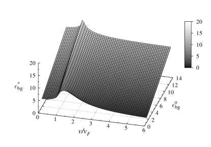
Figure 5: The reduced image force $F_{\text{i}}^{0}$ from the MDF-RPA model with vanishing damping ($\gamma=0$) for a proton ($Z=1$) moving over intrinsic graphene ($n=0$) on a substrate with dielectric constant $\epsilon_{\text{s}}$ and a zero gap ($h=0$). The force is expressed as an effective background dielectric constant $\epsilon_{\text{bg}}^{*}=1/\left[1+(4z_{0}^{2}/e^{2})\,F_{\text{i}}^{0}\right]$, and is shown as a function of the reduced proton speed $v/v_{F}$ and the actual background dielectric constant $\epsilon_{\text{bg}}^{0}=(\epsilon_{\text{s}}+1)/2$.

IV.3 Vanishing particle speed with a zero gap

In this subsection, we consider the density dependence of the stopping and image forces from the MDF-RPA model in the limit of vanishing particle speed ($v\rightarrow 0$) for a zero gap. For sufficiently small speeds, the inset in Fig. 1(a) shows that the stopping force is proportional to the particle speed $v$, and hence we can define a friction coefficient $\eta$ through the equation $F_{\text{s}}=-\eta v$. To evaluate $\eta$, it is sufficient to expand the loss function $\Im\!\left[-1/\epsilon(q,\omega)\right]$ to the first order in $\omega$ and use the resulting expression in Eq. (7) to find the stopping force. Alducin_2007 We find the expression for the continuum of low-energy, intra-band SPEs, subject to the constraint $q\leq 2k_{F}$, to be

$$-\Im\epsilon^{-1}(q,\omega)\approx\frac{2r_{s}}{\epsilon_{\text{bg}}^{0}\epsilon_{\text{TF}}^{2}(q)}\,\frac{\omega}{qv_{F}}\sqrt{\left(\frac{2k_{F}}{q}\right)^{2}-1},$$ (12)

where $\epsilon_{\text{TF}}(q)=1+q_{s}/q$ is the TF dielectric function. Ando_2006 ; Hwang_2007 ; Radovic_2008 The friction coefficient is then given by $\eta=2\pi\hbar\,nZ^{2}I(4z_{0}k_{F},r_{s})$, where the function $I(a,r_{s})$ is defined in Eq. (4) of Ref.Adam_2008

The case $z_{0}k_{F}\ll 1$ is particularly interesting because, unlike in the SCKE model, the constraint $q\leq 2k_{F}$ in Eq. (12) causes $I(4z_{0}k_{F},r_{s})$ to remain finite even as $z_{0}k_{F}\rightarrow 0$. Radovic_2008 The friction coefficient for a charge moving very close to graphene in the MDF-RPA model is therefore given by $\eta=2\pi\hbar\,nZ^{2}I(0,r_{s})$, and is proportional to the charge-carrier density $n$. In the opposite case, $z_{0}k_{F}\gg 1$, one recovers the TF result for the friction coefficient given in Eq. (37) of Ref.Radovic_2008 , which yields an asymptotic form $\eta=Z^{2}\hbar/(32z_{0}^{3}\sqrt{\pi n})$ that is independent of $v_{F}$. These two limiting cases for the friction coefficient can be observed in Fig. 2(a), which shows the MDF-RPA stopping forces for a particle speed $v=v_{F}/2$ that is very near the static limit. Recalling that the stopping force $F_{s}\approx-\frac{1}{2}v_{F}\eta$ is normalized by $F_{0}=Z^{2}e^{2}/(4z_{0}^{2})$ in Fig. 2(a), note that all MDF-RPA curves are proportional to $z_{0}^{2}$ for short distances and fall off as $z_{0}^{-1}$ for large distances. The transition between these two behaviours occurs around the peaks of the curves at $z_{0}k_{F}\sim 1$.

In the limit of vanishing particle speed, the image force is closely related to the well-studied problem of static screening of an external charge, for which the dielectric function in Eq. (2) reduces to $\epsilon(q,0)\equiv\epsilon_{\text{bg}}^{0}+\frac{2\pi e^{2}}{q}\Pi_{s}(q)$, where $\Pi_{s}(q)$ is the static MDF-RPA polarization function for graphene given in Appendix A. Ando_2006 ; Sarma_2007 ; Wunsch_2006 ; Hwang_2007 Although the $\omega$ integration in Eq. (8) is trivial with this dielectric function, the remaining $q$ integration cannot be completed analytically. However, expressions for the image force in the two limiting cases of $z_{0}k_{F}$ can be given explicitly. For $z_{0}k_{F}\ll 1$, the MDF-RPA image force reduces to the static limit for intrinsic graphene, $F_{\text{i}}^{0}=F_{0}\!\left[1/\!\left(\epsilon_{\text{bg}}^{0}+\frac{\pi}{2}\frac{v_{B}}{v_{F}}\right)-1\right]$. In the opposite case, $z_{0}k_{F}\gg 1$, one easily recovers the TF result for the static image force given in Eq. (38) of Ref.Radovic_2008 , which yields asymptotically $F_{\text{i}}\sim-F_{0}$. Fig. 2(b) clearly shows the transition between these two cases for the particle speed $v=v_{F}/2$, which is a good approximation to the static limit. Note that all normalized MDF-RPA image forces fall between the limits $\left(1+\frac{\pi}{2}\frac{v_{B}}{v_{F}}\right)^{-1}-1\approx-0.78$ and $-1$ in Fig. 2(a), with a broad transition occurring at $z_{0}k_{F}\sim 1$.

V MDF-RPA with finite damping

In this section, we use the MDF-RPA model with a finite damping rate $\gamma>0$ (by means of the Mermin dielectric function) to evaluate the stopping and image forces. Since the exact value of the damping rate is not known, we first treat it as a fitting parameter and come up with an estimate for $\gamma$ by comparing the MDF-RPA model with a finite damping rate to experimental data for the HREELS spectra of graphene on a SiC substrate. We then use this estimate to investigate the effects of the damping rate on the stopping and image forces for free graphene ($h\rightarrow\infty$), with a special focus on its role in the friction of low-speed particles.

It should be mentioned that introducing a finite $\gamma$ into the MDF-RPA dielectric function for graphene to create the Mermin dielectric function, $\epsilon_{M}(q,\omega,\gamma)$, is a non-trivial matter, as described in Appendix A. There is, however, a significant advantage in using such a dielectric function in numerical calculations of the stopping and image forces. Specifically, expressions for the MDF-RPA dielectric function in the strict $\gamma=0$ case make numerical integrations of Eqs. (7) and (8) difficult as the boundary of the integration domain, $0\leq\omega\leq qv$, intersects the delta-like plasmon line. A small but finite $\gamma$, however, broadens the plasmon line to allow for a simple numerical treatment of this delta-like behaviour. Throughout this paper, we have therefore reproduced the strict $\gamma=0$ limit of the MDF-RPA dielectric function Wunsch_2006 ; Hwang_2007 by using the value $\gamma=10^{-3}\times v_{F}k_{0}$, where $k_{0}=\sqrt{\pi n_{0}}$ and $n_{0}=10^{11}$ cm^-2.

V.1 Comparison with HREELS experiment

To obtain a reasonable estimate for $\gamma$, we compare the MDF-RPA model with finite damping to the experimental data of Liu et al. Liu_2008 for the HREELS spectra of graphene on a SiC substrate. Since the focus of this paper is on slow-moving particles that are unable to excite graphene’s $\sigma$ electrons, this HREELS experiment is more relevant to the present work than the EELS experiments on graphene and other carbon nanostructures. Stephan_2002 ; Kramberger_2008 ; Eberlein_2008 We note, however, that the effects of a SiC substrate on graphene are not as well understood as those of a SiO₂ substrate. Without entering the current debate, Trevisanutto_2008 ; Zhou_2007 we simply neglect any changes in graphene’s $\pi$-band structure that may result from a hybridization of its $\pi$ orbitals with the substrate and treat the gap height, $h$, as a free parameter.

Figure 6: The Mermin loss function (in arbitrary units) versus the energy loss for graphene with a charge-carrier density $n=2\times 10^{13}$ cm^-2) supported on a SiC substrate with static dielectric constant $\epsilon_{\text{s}}=9.7$ and a gap height $h$ = 1 Å. Model results are shown for damping rates $\hbar\gamma$ = 0, 200, and 400 meV, while symbols show the HREELS experimental data from Ref.Liu_2008

Since the measurements in Ref.Liu_2008 indicate that the maximum HREELS yields occur in the direction of near-specular reflection of slow incident electrons, it is appropriate to use Eq. (10) for the probability density of exciting the mode $(q,\omega)$. However, since we are not aware at this time of specific details of the experimental procedure that predominantly affect the low frequency range of the HREELS spectra via the prefactor in Eq. (10), Liu_2008 ; Ibach_1982 we simply focus on the Mermin loss function $\Im\!\left[-1/\epsilon_{M}(q,\omega,\gamma)\right]$ and assume that it gives the correct order of magnitude for spectral widths outside of this low frequency range. Therefore, in Fig. 6 we display a tentative comparison between the HREELS data Liu_2008 and the Mermin loss function with $\hbar\gamma=0$, 200, and 400 meV and a gap height of 1 Å for wavenumbers ranging from 0.008 to 0.102 Å^-1. The SiC subtrate is treated in the static mode with dielectric constant $\epsilon_{\text{s}}=9.7$, and the equilibrium density in graphene is set at $n=2\times 10^{13}$ cm^-2 (hence $\varepsilon_{F}\approx 570$ meV and $k_{F}\approx$ 0.08 Å^-1) to match experimental conditions. Note that since the HREELS data is scaled arbitrarily, the Mermin loss functions for $\hbar\gamma=200$ and 400 meV are scaled so that the maximum peak heights coincide with those from the experiment. For $\hbar\gamma=0$, however, the singular plasmon peak prevents such a scaling, and so the Mermin loss function is scaled by the same factor as for the $\hbar\gamma=400$ meV loss function.

In Fig. 6, the range $q\lesssim k_{F}$ is particularly interesting because the Mermin loss function with $\hbar\gamma=0$ exhibits three distinct features for these wavenumbers: a continuous spectrum of intra-band SPEs for $0<\omega<v_{F}q$, a continuous spectrum of inter-band SPEs for $\omega>v_{F}(2k_{F}-q)$, and a narrow plasmon line at $\omega=\omega_{p}(q)$ in the otherwise void interval $v_{F}q<\omega<v_{F}(2k_{F}-q)$. The fact that these three features are not visible in the experimental HREELS spectra can be tentatively explained by assuming that a large enough damping rate $\gamma$ exists, due to various scattering mechanisms, that a broadened plasmon line merges into the two regions of SPEs to form a single peak that follows approximately the original plasmon dispersion curve, $\omega=\omega_{p}(q)$. Note that a broadening of the plasmon line for the $\hbar\gamma=0$ loss function does occur for the wavenumbers $q=0.077$ and 0.102 Å^-1 as the plasmon line crosses the boundary $\omega=v_{F}(2k_{F}-q)$ and enters into the region of inter-band SPEs, in which collective plasma oscillations decay into SPEs in a way that can be described by a finite Landau damping rate, $\gamma_{L}$. Pines_1962 For the Mermin loss function with a phenomenological damping rate $\gamma$, however, a broadening of the plasmon line occurs for all $q$. Given that we have neglected the effects of temperature, the kinematic prefactor, and the reflection coefficient in Eq. (10), which all give rise to the low-frequency features in the HREELS spectra, Fig. 6 shows that a reasonably good qualitative agreement with the experiment can be achieved by using a gap height $h=1$ Å and a damping rate $\hbar\gamma=400$ meV.

Figure 7: The peak positions of the Mermin loss function shown as a function of the wavenumber $q/k_{F}$ for graphene with a charge-carrier density $n=2\times 10^{13}$ cm^-2 supported on a SiC substrate with static dielectric constant $\epsilon_{\text{s}}=9.7$. Model results are shown for damping rates $\hbar\gamma$ = 0, 200, and 400 meV, as well as for gap heights $h=0$ and 1 Å. Filled circles show the HREELS experimental data from Ref.Liu_2008

In Fig. 7, we compare the peak positions of the model spectra in Fig. 6 with the experimental HREELS data. Liu_2008 In addition to the best fit gap height $h=1$ Å, we also include the zero gap case to demonstrate the effect of the gap height. Note, however, that this effect is limited to shifting the spectral peak positions, and therefore does not significantly affect the estimate of the damping rate. In the long wavelength limit ($q\rightarrow 0$), it can be seen that the plasmon dispersion curve $\omega=\omega_{p}(q)$ for a vanishing damping rate exhibits the $\sqrt{q}$ behaviour of a classical 2D electron gas, Wunsch_2006 ; Hwang_2007 but as the damping rate increases the plasmon dispersion curve falls off in a more quasi-acoustic manner. It is worth noting, however, that none of the curves are able to describe the trend of the experimental data at long wavelengths. From Fig. 6, it can be seen that there is a strong coupling of graphene’s $\pi$ electron excitations with the non-dispersing Fuchs-Kliever surface phonon mode in the SiC substrate at the frequency $\approx$ 116 meV. Liu_2008 ; Nienhaus_1995 We note that a dynamic treatment of the substrate phonon excitation through Eq. (4), the use of a $q$-dependent damping rate, and the inclusion of low-frequency features through the prefactor in Eq. (10) may be necessary for accurate modeling of the experimental HREELS spectra in the full range of frequencies. However, further discussion on these points would go beyond the scope of the paper, and we merely conclude that a reasonable value for the damping rate $\hbar\gamma$ is on the order of several hundred meV.

V.2 Results for MDF-RPA with finite damping

In this subsection, we discuss the effects of a finite damping rate on the stopping and image forces calculated with the Mermin dielectric function for free graphene with several charge-carrier densities. Since it was found that a reasonable value for $\hbar\gamma$ is on the order of several hundred meV, we again consider the values $\hbar\gamma=0$, 200, and 400 meV, or equivalently $\gamma/(v_{F}k_{0})\approx 0$, 5, and 10, where $k_{0}=\sqrt{\pi n_{0}}$ and $n_{0}=10^{11}$ cm^-2.

Figure 8: The stopping force (a) and image force (b) from the MDF-RPA model with a finite damping rate shown as a function of the reduced speed $v/v_{F}$ of a proton ($Z=1$) moving at a distance $z_{0}$ = 20 Å above free graphene ($h\rightarrow\infty$). Results are shown for several values of the reduced damping rate $\gamma/(v_{F}k_{0})$, where $k_{0}=\sqrt{\pi n_{0}}$, and for several values of the reduced charge-carrier density $n/n_{0}$, where $n_{0}=10^{11}$ cm^-2.

In Fig. 8, we examine the velocity dependence of the stopping and image forces for the various damping rates and densities. For medium to high speeds ($v>v_{F}$), it can be seen that the strength of both forces decreases significantly as the damping rate increases, and that this effect diminishes faster for the image force than for the stopping force as the particle speed increases. For low speeds ($v<v_{F}$), the fact that the image force is unaffected by the damping rate can be understood through Eq. (21), from which it can be seen that the static limit of the Mermin polarization reduces to the static limit of the MDF-RPA polarization, $\Pi_{M}(q,0,\gamma)=\Pi_{s}(q)$.

Fig. 8(a) also shows an interesting relationship between the damping rate, $\gamma$, and the density, $n$, at low speeds. One can see that the strength of the stopping force tends to increase with $\gamma$ at a fixed density, but at a fixed $\gamma$ the stopping force tends to peak at some intermediate density. This trend is further confirmed in Fig. 9(a), which shows the stopping force as a function of the particle distance $z_{0}$ for low particle speeds. For high particle speeds, however, Fig. 9(b) shows that the distance dependence of the stopping force is affected more by the density than the damping rate.

Figure 9: The stopping force from the MDF-RPA model with a finite damping rate shown as a function of the distance $z_{0}$ of a proton ($Z=1$) moving at the low speed $v=v_{F}/2$ (a) and the moderately high speed $v=6v_{F}$ (b) above free graphene ($h\rightarrow\infty$). Results are shown for several values of the reduced damping rate $\gamma/(v_{F}k_{0})$, where $k_{0}=\sqrt{\pi n_{0}}$, and for several values of the reduced charge-carrier density $n/n_{0}$, where $n_{0}=10^{11}$ cm^-2.

V.3 Friction coefficient

The stopping forces in the inset of Fig. 8(a) suggest that, as for the case of vanishing damping, the concept of friction may be useful in the case of finite damping for low particle speeds. Again, we define the friction coefficient $\eta$ through the equation $F_{\text{s}}=-\eta v$. Although we wish to focus on the case of free graphene ($h\rightarrow\infty$), we provide analytic results for the slightly more general case of a zero gap and note that the case of free graphene can be recovered by taking $\epsilon_{\text{s}}=1$, and hence $\epsilon_{\text{bg}}^{0}=1$. To evaluate $\eta$, we expand the Mermin loss function for a zero gap to the first order in $\omega$, which gives

$$-\Im\epsilon_{M}^{-1}(q,\omega,\gamma)\approx\frac{\omega}{\gamma}\frac{2\pi e^{2}}{q}\frac{\Pi_{s}(q)}{\left[\epsilon_{\text{bg}}^{0}+\frac{2\pi e^{2}}{q}\Pi_{s}(q)\right]^{2}}\left[-1+\frac{\Pi_{s}(q)}{\Pi(q,i\gamma)}\right],$$ (13)

Eq. (13) can then be substituted into the stopping force, Eq. (7), to get an expression for the friction coefficient. Since the resulting integral cannot be evaluated analytically for an arbitrary density $n$, we first consider the case of intrinsic graphene ($n=0$), for which

$$\Pi(q,i\gamma)=\frac{1}{4\hbar}\frac{q^{2}}{\sqrt{\gamma^{2}+\left(qv_{F}\right)^{2}}},$$ (14)

and hence $\Pi_{s}(q)=q/(4\hbar v_{F})$. Using these expressions in Eq. (13), the friction coefficient for intrinsic graphene is given by

$$\eta_{0}=\frac{\pi Z^{2}e^{2}}{4\zeta_{0}v_{F}}\left(\frac{\gamma}{v_{F}}\right)^{2}\frac{\frac{\pi}{2}\frac{v_{B}}{v_{F}}}{\left(\epsilon_{\text{bg}}^{0}+\frac{\pi}{2}\frac{v_{B}}{v_{F}}\right)^{2}}\times$$

$$\left[-\frac{1}{2\pi\zeta_{0}}+Y_{0}(\zeta_{0})-Y_{1}(\zeta_{0})-H_{0}(\zeta_{0})+H_{1}(\zeta_{0})\right],$$ (15)

where $\zeta_{0}\equiv 2z_{0}\gamma/v_{F}$, and $Y_{\nu}$ and $H_{\nu}$ are the Bessel function of the second kind and the Struve function, respectively. By combining the leading terms of the series expansions for large and small $\zeta_{0}$ in this expression for $\eta_{0}$, one obtains the simple but surprisingly accurate formula (with a maximum error of approximately 3% at $\zeta_{0}\approx 1$)

$$\eta_{0}\approx\frac{Z^{2}e^{2}}{8v_{F}}\frac{\frac{\pi}{2}\frac{v_{B}}{v_{F}}}{\left(\epsilon_{\text{bg}}^{0}+\frac{\pi}{2}\frac{v_{B}}{v_{F}}\right)^{2}}\frac{1}{z_{0}\!\left(z_{0}+\frac{v_{F}}{\gamma}\right)}.$$ (16)

We now consider the friction coefficient $\eta$ for an arbitrary density $n$. In Fig. 10, we display the normalized friction coefficient $\eta/\eta_{0}$ for free graphene ($\epsilon_{\text{bg}}=1$) as a function of the reduced damping rate $\gamma/(v_{F}k_{0})$, where $k_{0}=\sqrt{\pi n_{0}}$, and the reduced charge-carrier density $n/n_{0}$, where $n_{0}=10^{11}$ cm^-2. It can be seen that the friction coefficient for a slow particle moving at a distance $z_{0}$ = 20 Å above free graphene is a rather complicated function of $\gamma/(v_{F}k_{0})$ and $n/n_{0}$, but the qualitative behaviour of this function can be understood. Recall from subsection III.C that the friction coefficient for a vanishing damping rate goes as $\eta\propto n$ for $z_{0}k_{F}\ll 1$ and as $\eta\propto 1/(z_{0}^{3}n)$ for $z_{0}k_{F}\gg 1$, where $k_{F}=\sqrt{\pi n}$. For the distance $z_{0}=20$ Å, the transition between these two limiting behaviours occurs at $n/n_{0}\approx 80$. For a finite damping rate, we find in Eq. (16) that the friction coefficient goes as $\eta\propto\gamma/(z_{0}v_{F})$ for $z_{0}\gamma/v_{F}\ll 1$ and as $\eta\propto z_{0}^{-2}$ for $z_{0}\gamma/v_{F}\gg 1$. For the distance $z_{0}$ = 20 Å, the transition between these two limiting behaviours occurs at $\gamma/(v_{F}k_{0})\approx 9$. Note how a saddle point develops at these two values for the density and damping rate in the surface plotted in Fig. 10.

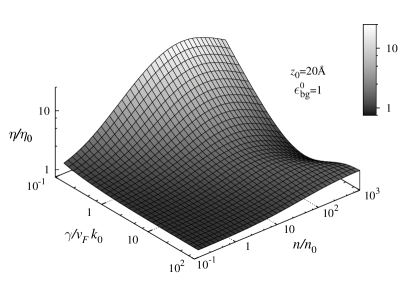
Figure 10: The friction coefficient $\eta$ normalized by the friction coefficient for intrinsic graphene $\eta_{0}$ and shown as a function of the reduced damping rate $\gamma/(v_{F}k_{0})$, where $k_{0}=\sqrt{\pi n_{0}}$, and the reduced charge-carrier density $n/n_{0}$, where $n_{0}=10^{11}$ cm^-2, for a proton ($Z=1$) moving at a distance $z_{0}=20$Å above free graphene ($\epsilon_{\text{bg}}^{0}=1$).

VI Concluding remarks

We have presented an extensive analysis of the stopping and image forces on an external point charge moving parallel to a single layer of supported, doped graphene under conditions validating the massless Dirac fermion (MDF) representation of graphene’s $\pi$ electron band excitations. These conditions require that the particle distance, $z_{0}$, be greater than the lattice constant of graphene, and that the particle speed, $v$, satisfy $\hbar v/z_{0}<$ 2 eV. Calculations of the velocity and distance dependencies of the stopping and image forces were performed within the random phase approximation (RPA) for a broad range of charge-carrier densities with three major goals: to compare the results with a semi-classical kinetic equation (SCKE) model, to examine of the effects of a finite graphene-substrate gap, and to explore the effects of a finite damping rate introduced using Mermin’s procedure.

With respect to the first goal, a comparison of the forces from the MDF-RPA and SCKE models in the regime of vanishing damping has revealed that the latter model may be justified for particle distances satisfying $z_{0}k_{F}>1$ for $v<v_{F}$ and satisfying $z_{0}k_{F}\gg 1$ for $v>v_{F}$. When combined through Bohr’s adiabatic criterion, these conditions suggest that the SCKE model is valid only for heavily doped graphene with $\varepsilon_{F}>\hbar v/z_{0}$, for which the effects of the inter-band single-particle excitations on the stopping and image forces are minimized. With respect to the second goal, the effects of a finite gap between graphene and a supporting substrate in the MDF-RPA model with vanishing damping have been found to be quite strong, particularly for medium to high particle speeds. These results have confirmed earlier findings from the SCKE model Radovic_2008 and raise some concern over the common practice of treating graphene with a zero gap when dealing with the dynamic-polarization forces on external moving charges. With respect to the third goal, we have made an effort to estimate the order of magnitude of the damping rate, $\gamma$, by providing a tentative fit of the MDF-RPA dielectric function modified by Mermin’s procedure with recently published experimental data for the HREELS spectra of graphene on a SiC substrate. Liu_2008 To the best of our knowledge, this experiment is the only one that has been performed under the parameter constraints of our model. With a suitable estimate of $\gamma$, we have found that both the stopping and image forces are primarily affected by the damping rate at moderate particle speeds. We have also shown that the combined effect of a finite gap and a finite damping rate can be important in modeling the plasmon peak positions of the Mermin loss function.

In all calculations of the stopping and image forces within the MDF-RPA model, we have also found strong effects of the charge-carrier density, $n$, which are only weakened at sufficiently high particle speeds ($v\gg v_{F}$). Although both forces were shown to approach the results for intrinsic graphene in this regime, it is likely that the diminished effect of graphene’s doping level will be masked by excitations of graphene’s $\sigma$ electrons as $\hbar v/z_{0}$ exceeds the $\sigma$ band gap ($\sim$ 7 eV). On the other hand, the parameter ranges considered in this paper are perfectly suitable for studying the friction of slow charges moving near graphene. The friction coefficient’s dependence on the particle distance, the charge-carrier density, and the damping rate have been studied in detail for a zero gap, where analytic or semi-analytic results have been obtained. An intricate relationship has been found between these parameters and the friction coefficient, which may be of great practical interest for applications involving the concept of friction, including surface processing and electrochemistry with graphene.

There are several possible routes for extending the present work. Although not addressed in this paper, we have examined the local field correction to the MDF-RPA dielectric function at the level of Hubbard approximation Adam_2009 and found no significant effects on the stopping and image forces. However, a recent treatment of the local field effects (LFE) using the $GW$ method has led to significant improvements in the loss function of free, undoped graphene in the MDF-RPA model with vanishing damping. Trevisanutto_2008 Therefore, it would be desirable to treat the LFE using the $GW$ method and explore its effects on the stopping and image forces. Furthermore, it would be desirable to extend the domain of applicability of the MDF-RPA model to small particle distances by including the finite size of graphene’s $\pi$ orbitals. Shung_1986 Finally, the results of our tentative comparison of the Mermin loss function and the experimental HREELS spectra for graphene on a SiC substrate have opened up the possibility of further modeling of this data in the low frequency regime.

Appendix A The Mermin dielectric function

In this appendix, we extend the MDF-RPA dielectric function for graphene given in Refs. Hwang_2007, and Wunsch_2006, to include a finite damping rate $\gamma>0$. Beginning with Eq. (3) of Hwang and Das Sarma, Hwang_2007 we rewrite the polarization as $\Pi(q,\omega+i\gamma)=\Pi^{-}(q,\omega+i\gamma)+\Pi^{+}(q,\omega+i\gamma)$, where it is assumed that $q>0$ and $\omega>0$. For a finite damping rate, the term $\Pi^{-}(q,\omega+i\gamma)$ is given by

$$\Pi^{-}(q,\omega+i\gamma)=\frac{g_{s}g_{v}qi}{16\hbar v_{F}\sqrt{\zeta}},$$ (17)

where

$$\zeta\equiv\left(\frac{\omega+i\gamma}{v_{F}q}\right)^{2}-1.$$ (18)

Note that the square root of a complex number $z$ is defined as $\sqrt{z}=e^{\frac{1}{2}\log z}$, where $\log z=\log|z|+i\arg z$ and the argument, $\arg z$, is defined up to an integer multiple of $2\pi$. As with other multi-valued complex functions, the square root must be evaluated with respect to a single-valued branch, for which the value of $\arg z$ is selected from an interval of length $2\pi$. For instance, the principal branch, denoted $\text{Arg }z$, selects the value of $\arg z$ from the interval $(-\pi,\pi]$. In Eq. (17), the square root must be evaluated with respect to the branch of $\arg z$ that selects values from $(\theta-2\pi,\theta]$, where $\theta\equiv\text{Arg }\zeta$ is the principal argument of $\zeta$.

The term $\Pi^{+}(q,\omega+i\gamma)$ is given by

$$\Pi^{+}(q,\omega+i\gamma)=\frac{g_{s}g_{v}k_{F}}{2\pi\hbar v_{F}}+\frac{g_{s}g_{v}q}{16\pi\hbar v_{F}\sqrt{\zeta}}\times$$

$$\left[F\!\left(\frac{\omega+i\gamma}{v_{F}q}+\frac{2k_{F}}{q}\right)-F\!\left(\frac{\omega+i\gamma}{v_{F}q}-\frac{2k_{F}}{q}\right)\right],$$ (19)

where

$$F(u)\equiv\frac{u\sqrt{\zeta(u^{2}-1)}}{\sqrt{\zeta}}-\log\left(u\sqrt{\zeta}+\sqrt{\zeta(u^{2}-1)}\right)$$ (20)

and $\zeta$ is defined in Eq. (18). The square roots and logarithms in Eqs. (A) and (20) must also be evaluated with respect to the branch of $\arg z$ that selects values from $(\theta-2\pi,\theta]$, where $\theta=\text{Arg }\zeta$. Note that $\sqrt{\zeta(u^{2}-1)}\neq\sqrt{\zeta}\sqrt{u^{2}-1}$ when dealing with specific branches of the square root, so Eq. (20) cannot be simplified in the obvious manner.

After introducing a finite damping rate $\gamma$, it is necessary to modify the polarization $\Pi(q,\omega+i\gamma)$ using Mermin’s procedure to conserve the local number of charge carriers in graphene.Mermin_1970 ; Qaiumzadeh_2008 The Mermin polarization function is then given by

$$\Pi_{M}(q,\omega,\gamma)=\frac{\Pi(q,\omega+i\gamma)}{1-\displaystyle{\frac{i\gamma}{\omega+i\gamma}\left[1-\frac{\Pi(q,\omega+i\gamma)}{\Pi_{s}(q)}\right]}},$$ (21)

where $\Pi_{s}(q)\equiv\Pi(q,0)$ is the static limit of the polarization $\Pi(q,\omega+i\gamma)$ with $\omega\rightarrow 0$ and $\gamma\rightarrow 0$, given by Wunsch_2006 ; Hwang_2007

$$\Pi_{s}(q)=\frac{g_{s}g_{v}k_{F}}{2\pi\hbar v_{F}}\times$$

$$\left\{\begin{array}[]{ll}1&\text{if }q\leq 2k_{F}\\ 1-\frac{1}{2}\sqrt{1-\frac{4k_{F}^{2}}{q^{2}}}-\frac{q}{4k_{F}}\arcsin{\left(\frac{2k_{F}}{q}\right)+\frac{\pi q}{8k_{F}}}&\text{otherwise}\\ \end{array}\right\}.$$ (24)

Note that the piecewise definition of Eq. (A) ensures that the square root and arcsine are real-valued. Using Eq. (21) in Eq. (2), the Mermin dielectric function is then given by

$$\epsilon_{M}(q,\omega,\gamma)=\epsilon_{\text{bg}}(q)+\frac{2\pi e^{2}}{q}\Pi_{M}(q,\omega,\gamma).$$ (25)

In the limit $\gamma\rightarrow 0$, it can be shown that Eq. (25) is equivalent to the dielectric functions presented in Refs.Wunsch_2006 ; Hwang_2007 † The difficulty in obtaining a compact form for the dielectric function in the limit as $\gamma\rightarrow 0$ lies in reproducing the behaviour of the branch cut that naturally arises for $\gamma>0$ — it is necessary to employ rather complicated piecewise-defined functions, as in Refs.Hwang_2007 ; Wunsch_2006 Alternatively, the compact Eq. (25) may be used with a small, positive $\gamma$ to approximate this limit, or Eq. (25) may be used with a realistic damping rate, $\gamma$, as originally intended. To this end, we describe how to implement the branch cut technique below.

Most computer codes support basic arithmetic for complex numbers including exponentiation with base $e$, but only include built-in functions for computing complex logarithms and square roots with respect to the principal branch. To compute logarithms and square roots with respect to the branch required in Eqs. (17), (A), and (20), it is necessary to implement a function argbranch(z) that returns the argument of a complex number z in the range $(\theta-2\pi,\theta]$, where $\theta=\text{Arg }\zeta$. Using the built-in function atan2(y,x), which returns the polar angle of the Cartesian point (x,y) in the range $(-\pi,\pi]$, one may define

$$\texttt{Arg(z)}:\texttt{z}\mapsto\texttt{atan2(Im(z),Re(z)),}$$ (26)

$$\texttt{argbranch(z)}:$$

$$\texttt{z}\mapsto\left\{\begin{array}[]{ll}\texttt{Arg(z)}-\texttt{2}\pi&\text{if }\texttt{Arg(z)}>\texttt{Arg($\zeta$)}\\ \texttt{Arg(z)}&\text{otherwise}\end{array}\right..$$ (29)

Since $q>0$ and $\omega>0$, Eq. (A) correctly handles all values of z. The functions for the corresponding branches of the logarithm and the square root are then defined as

$$\texttt{logbranch(z)}:\texttt{z}\mapsto\texttt{log(|z|)}+i\texttt{argbranch(z)},$$ (30)

$$\texttt{sqrtbranch(z)}:\texttt{z}\mapsto\texttt{exp(logbranch(z)/2)},$$ (31)

where |z| is the modulus of z, log() and sqrt() are the real-valued logarithm and square root, respectively, and exp() is the complex exponentiation with base $e$. It is then a simple matter of evaluating Eqs. (17), (A), and (20) with respect to these branches of the logarithm and square root. Note that argbranch($\zeta$) must return Arg($\zeta$) to yield the correct result.

References

- (1) O. Stephan, D. Taverna, M. Kociak, K. Suenaga, L. Henrard, and C. Colliex, Phys. Rev. B 66, 155 422 (2002).
- (2) C. Kramberger, R. Hambach, C. Giorgetti, M. H. R mmeli, M. Knupfer, J. Fink, B. B chner, L. Reining, E. Einarsson, S. Maruyama, F. Sottile, K. Hannewald, V. Olevano, A. G. Marinopoulos, and T. Pichler, Phys. Rev. Lett. 100, 196803 (2008).
- (3) T. Eberlein, U. Bangert, R.R. Nair, R. Jones, M. Gass, A.L. Bleloch, K.S. Novoselov, A. Geim, and P.R. Briddon, Phys. Rev. B 77, 233406 (2008).
- (4) P. E. Trevisanutto, C. Giorgetti, L. Reining, M. Ladisa, and V. Olevano, Phys. Rev. Lett. 101, 226405 (2008).
- (5) D. Taverna, M. Kociak, V. Charbois, and L. Henrard, Phys. Rev. B 66, 235419 (2002).
- (6) D.J. Mowbray, Z.L. Miskovic, F.O. Goodman, and Y.-N. Wang, Phys. Rev. B 70, 195418 (2004); ibid. D.J. Mowbray, Z.L. Miskovic, and F.O. Goodman, Phys. Rev. B 74, 195435 (2006).
- (7) I. Radovic, Lj. Hadzievski, N. Bibic, and Z.L. Miskovic, Phys. Rev. A 76, 042901 (2007).
- (8) B. Diaconescu, K. Pohl, L. Vattuone, L. Savio, P. Hofmann, V. M. Silkin, J. M. Pitarke, E. V. Chulkov, P. M. Echenique, D. Far as, and M. Rocca, Nature 448, 57 (2007).
- (9) M. Alducin, V.M. Silkin, and J.I. Juaristi, Nucl. Instrum. Methods B 256, 383 (2007).
- (10) V.M. Silkin, M. Alducin, J.I. Juaristi, E.V. Chulkov, and P.M. Echenique, J. Phys.: Condens. Matter 20, 304209 (2008).
- (11) Y. Liu, R.F. Willis, K.V. Emtsev, and Th. Seyller, Phys. Rev. B 78, 201403(R) (2008).
- (12) K.S. Novoselov, A. K. Geim, S. V. Morozov, D. Jiang, M. I. Katsnelson, I. V. Grigorieva, S. V. Dubonos, and A. A. Firsov, Nature 438, 197 (2005).
- (13) T. Ando, J. Phys. Soc. Japan 75, 074716 (2006).
- (14) T. Stauber, N.M.R Peres, and F. Guinea, Phys. Rev. B 76, 205423 (2007).
- (15) E.H. Hwang, S. Adam, and S. Das Sarma, Phys. Rev. Lett. 98, 186806 (2007).
- (16) S. Adam, E.H. Hwang, V.M, Galitskii, and S. Das Sarma, Proc. Natl. Acad. USA 104, 18392 (2007).
- (17) S. Adam and S. Das Sarma, Solid State Communications 146, 356 (2008).
- (18) J.H. Chen, C. Jang, S. Adam, M.S. Fuhrer, E.D. Williams, and M. Ishigami, Nature Physics 4, 377 (2008).
- (19) A. H. Castro Neto, F. Guinea, N. M. Peres, K. S. Novoselov, and A. K. Geim, Rev. Mod. Phys. 81, 109 (2009).
- (20) K. W.-K. Shung, Phys. Rev. B 34, 979 (1986).
- (21) B. Wunsch, T. Stauber, F. Sols, and F. Guinea, New Journal of Physics 8, 318 (2006).
- (22) E.H. Hwang and S. Das Sarma, Phys. Rev. B 75, 205418 (2007).
- (23) Y. Barlas, T. Pereg-Barnea, M. Polini, R. Asgari, and A.H. MacDonald, Phys. Rev. Lett. 98, 236601 (2007).
- (24) M. Khantha, N.A. Cordero, L.M. Molina, J.A. Alonso, and L.A. Girifalco, Phys. Rev. B 70, 125422 (2004).
- (25) S. Tomassone and A. Widom, Phys. Rev. B 56, 4938 (1997).
- (26) G.V. Dedkov and A.A. Kyasov, Nucl. Instrum. Methods B 237, 507 (2005).
- (27) M.Z. Bazant and T.M. Squires, Phys. Rev. Lett. 92, 066101 (2004).
- (28) H.H. Brongersma, M. Draxler, M. de Ridder, and P. Bauer, Surf. Sci. Repts. 62, 63 (2007).
- (29) A.V. Krasheninnikov and K. Nordlund, Phys. Rev. B 71, 245408 (2005); C.S. Moura and L. Amaral, J. Phys. Chem. B 109, 13515 (2005); W. Zhang, Z. Zhu, Z. Xu, Z. Wang, and F. Zhang, Nanotechnology 16, 2681 (2005); Z.L. Miskovic, Radiation Effects and Defects in Solids 162, 185 (2007).
- (30) G. Ramos and B.M.U. Scherzer, Nucl. Instrum. Methods B 85, 479 (1994); ibid. 174, 329 (2001).
- (31) E. Yagi, T. Iwata, T. Urai and K. Ogiwara, J. Nucl. Mater. 334, 9 (2004).
- (32) S. Cernusca, M. Fürsatz, HP. Winter and F. Aumayr, Europhys. Lett. 70, 768 (2005).
- (33) H. Winter, Phys. Rep. 367, 387 (2002).
- (34) G. Gumbs, D. Huang, and P. M. Echenique, Phys Rev. B 79, 035410 (2009).
- (35) P.M. Echenique and A. Howie, Ultramicroscopy 16, 269 (1985).
- (36) Ph. Lambin, A.A. Lucas, and J.P. Vigneron, Surf. Sci. 182, 567 (1987).
- (37) T. Inaoka, Surf. Sci. 493, 687 (2001).
- (38) Y.-H. Song, Y.-N. Wang, Z.L. Miskovic, Phys. Rev. A 63, 052902 (2001).
- (39) Y.-H. Song, Y.-N. Wang, Z.L. Miskovic, Phys. Rev. A 72, 012903 (2005).
- (40) D.-P. Zhou, Y.-N. Wang, L. Wei, and Z.L. Miskovic, Phys. Rev. A 72, 023202 (2005).
- (41) D. Borka, S. Petrovic, N. Neskovic, D.J. Mowbray, and Z.L. Miskovic, Phys. Rev. A 73, 062902 (2006); D. Borka, D.J. Mowbray, Z.L. Miskovic, S. Petrovic, and N. Neskovic, ibid. 77, 032903 (2008).
- (42) D.-P. Zhou, Y.-H. Song, Y.-N. Wang, and Z.L. Miskovic, Phys. Rev. A 73, 033202 (2006).
- (43) D.J. Mowbray, S. Chung, Z.L. Miskovic, and F.O. Goodman, Nanotechnology 18, 424034 (2007).
- (44) M. Fritz, K. Kimura, H. Kuroda, and M. Mannami, Phys. Rev. A 54, 3139 (1996).
- (45) J. I. Juaristi, A. Arnau, P. M. Echenique, C. Auth and H. Winter, Phys. Rev. Lett. 82, 1048 (1999).
- (46) I. Radovic, Lj. Hadzievski, and Z.L. Miskovic, Phys. Rev. B 77, 075428 (2008).
- (47) V. Ryzhii, A. Satou, and T. Otsuji, J. Appl. Phys. 101, 024509 (2007).
- (48) O. Vafek, Phys. Rev. Lett. 97, 266406 (2006).
- (49) C. Jang, S. Adam, J.-H. Chen, E. D. Williams, S. Das Sarma, and M. S. Fuhrer, Phys. Rev. Lett. 101, 146805 (2008).
- (50) N.D. Mermin, Phys. Rev. B 1, 2362 (1970).
- (51) R. Asgari, M. M. Vazifeh, M. R. Ramezanali, E. Davoudi, and B. Tanatar, Phys. Rev. B 77, 125432 (2008); A. Qaiumzadeh, N. Arabchi, R. Asgari, Solid State Communications 147, 172 (2008).
- (52) E.H. Hwang and S. Das Sarma, Phys. Rev. B 77, 195412 (2008).
- (53) M. V. Fischetti, D. A. Neumayer, and E. A. Cartier, J. Appl. Phys. 90, 4587 (2001).
- (54) S. Fratini and F. Guinea, Phys. Rev. B 77, 195415 (2008).
- (55) H. Ibach and D. L. Mills, Electron Energy Loss Spectroscopy and Surface Vibrations, Academic Press, New York, 1982.
- (56) G. Barton, Rep. Prog. Phys. 42, 963 (1979).
- (57) A.A. Lucas, Phys. Rev. B 20, 4990 (1979).
- (58) M. Ishigami, J. H. Chen, W. G. Cullen, M. S. Fuhrer, and E. D. Williams, Nano Lett. 7, 1643 (2007).
- (59) H. E. Romero, N. Shen, P. Joshi, H. R. Gutierrez, S. A. Tadigadapa, J. O. Sofo, and P. C. Eklund, ACS Nano 2, 2037 (2008).
- (60) S. Y. Zhou, G.-H. Gweon, A. V. Fedorov, P. N. First, W. A. de Heer, D.-H. Lee, F. Guinea, A. H. Castro Neto, and A. Lanzara, Nature Materials 6, 770 (2007); E. Rotenberg, A. Bostwick, T. Ohta, J. L. McChesney, T. Seyller, and K Horn, ibid. Nature Materials 7, 258 (2008); S.Y. Zhou, D.A. Siegel, A.V. Fedorov, F.El Gabaly, A.K. Schmid, A.H. Castro Neto, D.-H. Lee, and A. Lanzara, ibid. Nature Materials 7, 259 (2008).
- (61) D. Pines and J. R. Schrieffer, Phys. Rev. 125, 804 (1962).
- (62) H. Nienhaus, T. U. Kampen, and W. Mönch, Surf. Sci. 324, L238 (1995).
- (63) S. Adam, E. H. Hwang, E. Rossi, and S. Das Sarma, Solid State Communications 149, 1072 (2009).
- (64) Ref. Hwang_2007 appears to contain a typographical error: Eq. (12) should take the absolute value of the entire argument to ln, not just the denominator. With this correction, the dielectric functions are equivalent.