Time Evolution of the 3-D Accretion Flows: Effects of the Adiabatic Index and Outer Boundary Condition

Abstract

We study a slightly rotating accretion flow onto a black hole, using the fully three dimensional (3-D) numerical simulations. We consider hydrodynamics of an inviscid flow, assuming a spherically symmetric density distribution at the outer boundary and a small, latitude-dependent angular momentum. We investigate the role of the adiabatic index and gas temperature, and the flow behaviour due to non-axisymmetric effects. Our 3-D simulations confirm axisymmetric results: the material that has too much angular momentum to be accreted forms a thick torus near the equator and the mass accretion rate is lower than the Bondi rate. In our previous study of the 3-D accretion flows, for $\gamma=5/3$, we found that the inner torus precessed, even for axisymmetric conditions at large radii. The present study shows that the inner torus precesses also for other values of the adiabatic index: $\gamma=4/3,1.2$, and 1.01. However, the time for the precession to set increases with decreasing $\gamma$. In particular, for $\gamma=1.01$ we find that depending on the outer boundary conditions, the torus may shrink substantially due to the strong inflow of the non-rotating matter and the precession will have insufficient time to develop. On the other hand, if the torus is supplied by the continuous inflow of the rotating material from the outer radii, its inner parts will eventually tilt and precess, as it was for the larger $\gamma$’s.

1 Introduction

The black holes capturing the gas from their vicinity are ubiquitous in the Universe, and accretion onto the central black hole is the source of energy that powers the brightest sources on our sky, from quasars, through the gamma ray bursts, to the X-ray binaries. The fast rotation of material before it becomes captured by the central object leads to the formation of a thin accretion disk, where the gravitational energy is effectively dissipated through the viscous stresses and radiated away in the form of high energy radiation. On the other hand, if the gas does not rotate, or rotates very slowly, the viscous disk does not form and the material falls radially onto the center. The rate of accretion is then equal to the Bondi accretion rate, derived analytically (Bondi 1952). The flows with a small, latitude dependent angular momentum were studied numerically e.g. in Proga & Begelman (2003a,b) in 2D, and Janiuk et al. (2008) in 3D, and showed that in this case the accretion rate is on the order of 20-30% of the Bondi rate. The astrophysical situation that may be described by such solutions is the radiatively inefficient flow of gas captured by the supermassive black holes in low luminosity AGNs, or the quiescent state of an X-ray binary.

The simulations show, that if the torus is formed due to rotation, the gas cannot accrete unless some angular momentum transport mechanism is introduced. Therefore no accretion proceeds close to and through the equatorial plane, and the material accumulated in this region either flows out due to the centrifugal forces and gas pressure, or eventually turns to smaller latitudes and flows radially through the polar region. The recent three dimensional studies showed, that in the latter case the amount of gas turning in the direction above or below the torus may depend on the azimuth, and in consequence lead to the tilt of this torus and its precession.

The present work is an extension of the previous study (Janiuk et al. 2008) to check how the gas properties, described by its equation of state, will influence the results. The general form of the EOS assumed here is the polytropic relation, and the index of $\gamma=5/3$, appropriate for gas pressure dominated system, is well suited for example in the inactive AGNs. On the other hand, the GRBs, which result from accretion of the massive stellar envelope, being a mixture of nucleons, neutrinos, electron-positron pairs and trapped photons (e.g. Janiuk et al. 2004; 2007), will rather be better described by a relativistic EOS with $\gamma=4/3$, than the ideal gas EOS. The still smaller values of $\gamma$, discussed in Mościbrodzka & Proga (2008), can account for the nearly isothermal gas, suggested to constitute the protogalactic disks.

Therefore we consider here the 3-dimensional hydrodynamical models with a range of $\gamma$ indices describing different gas microphysics. We concentrate on the initially axisymmetric conditions, which were shown to produce the non-axisymmetric results in the process of time evolution. The content of the article is as follows. In Section 2, we describe the method used in our calculations, to determine the initial conditions and subsequent evolution of the flow. In Section 3, we present the simulations results for the 3-D models with various adiabatic indices (Sec. 3.1). We discuss the torus precession and the influence of the outer boundary conditions (Sec. 3.2), which occured to be important, especially for models with smaller $\gamma$. The models with various gas temperatures are presented in Sec. 3.3. We discuss our results in Section 4.

2 Method

2.1 Initial conditions

In the analytical formula of Bondi (1952), the steady state solution to the equations of mass and angular momentum conservation is parameterized with the two quantities at infinity: density, $\rho_{\infty}$, and sound speed, $c_{\rm s,\infty}$. The solution is given by the accretion rate of:

$$\dot{M}_{\rm B}=\lambda 4\pi R_{\rm B}^{2}\rho_{\infty}c_{\rm s,\infty}$$ (1)

where the dimensionless parameter $\lambda$ depends only on the adiabatic index:

$$\lambda={1\over 4}{2\over(5-3\gamma)}^{(5-3\gamma)\over 2(\gamma-1)}$$ (2)

for $1<\gamma<5/3$. In the limit of $\gamma\rightarrow 1.0$, this parameter approaches:

$$\lambda={1\over 4}\exp(3/2),$$ (3)

while in the limit of $\gamma=5/3$ the accretion rate is calculated from the transonic solution in the pseudonewtonian potential, PW, (Paczyński & Wiita 1980), and depends on the sound speed at infinity (see Proga & Begelman 2003a for the derivation from the density and sound speed at the sonic radius):

$$\lambda={9\over 4}[{c_{\rm s,\infty}\over c}(1+{1\over\sqrt{3}}{c\over c_{\rm s,\infty}})]^{4}.$$ (4)

The Bondi radius is equal to

$$R_{\rm B}={GM\over c_{\rm s,\infty}^{2}}.$$ (5)

The transonic solution is obtained for $\gamma<5/3$ in the Newtonian potential, and the sonic radius is located at:

$$r_{\rm s}={GM\over 2c_{\rm s}^{2}(r_{\rm s})}$$ (6)

with the sound speed in the sonic radius equal to:

$$c_{\rm s}(r_{\rm s})=c_{\rm s,\infty}\sqrt{2\over 5-3\gamma}.$$ (7)

The above relation gives no sonic point for $\gamma=5/3$, and in this case the transonic solution is found for the PW potential, with the sonic radius equal to:

$$r_{\rm s}={GM\over c^{2}}+\sqrt{2\over 3}{GM\over c_{\rm s,\infty}c}.$$ (8)

We model the initial conditions for the spherically symmetric Bondi inflow, solving iteratively the Bernoulli equation in 1-D:

$$B=H+{v_{\rm r}^{2}\over 2}+\Phi$$ (9)

where

$$\Phi=-{GM\over r-R_{\rm S}}$$ (10)

is the PW potential, $R_{\rm S}=2GM/c^{2}$ is the Schwarzschild radius, and

$$H={1\over\gamma-1}c_{\rm s,\infty}^{2}[({\rho\over\rho_{\infty}})^{\gamma-1}-1]$$ (11)

is the enthalpy.

We parameterize our model with $\rho_{\infty}$ and $c_{\rm s,\infty}$. The latter is conveniently used to define a dimensionless radius, $R_{\rm S}^{{}^{\prime}}=R_{\rm S}/R_{\rm B}=2c_{\rm s,\infty}^{2}/c^{2}$. Depending on $\gamma$, we calculate the dimensionless accretion rate from Eq. 2, Eq. 3, or Eq. 4. Then, we solve for the density profile, while the velocity is found from the continuity equation:

$$\dot{M}_{\rm B}=-4\pi r^{2}v_{\rm r}\rho.$$ (12)

In the initial condition, we also impose a slight rotation of the outermost parts of the Bondi flow. This is done by means of the latitude-dependent angular momentum,

$$l=l_{0}(1-|\cos\theta|)$$ (13)

where $l_{0}$ is a dimensionless parameter, which corresponds to the circularization radius $R_{\rm C}$ (i.e. the radius at which $GM/r^{2}=v_{\phi}^{2}/r$). Therefore, our initial velocity $v_{\theta}$ is everywhere equal to 0.0, whereas the velocity $v_{\phi}$ is initially non-zero only in a fixed, quasi-conical region, with its radial extension limited by the sound speed at infinity. This region is defined as follows:

$$v_{\phi}=\left\{\begin{array}[]{ll}0&{\rm for}~{}~{}\,~{}~{}|v_{\rm r}|>c_{\rm s,\infty}{}{}{}{}\\ \sqrt{R_{C}}R_{B}c_{\rm s,\infty}{1-|\cos{\theta}|\over r\sin{\theta}}&{\rm for}~{}~{}\,~{}~{}|v_{\rm r}|<c_{\rm s,\infty}\end{array}\right.$$ (14)

2.2 Boundary conditions

The boundary conditions are set at the outer radius of the computational domain. We impose a spherically symmetric outer boundary condition for the flow density, $\rho(r_{\rm out})$, and energy density, $e(r_{\rm out})$, to be equal to these quantities determined from the initial analytical soulution for the Bondi flow. Because the outer radius of our grid is finite, the density at the outer edge is not exactly equal to $\rho_{\infty}$, but roughly twice larger. Nevertheless, the outer radius of 1.2 $R_{\rm B}$ is sufficient and such a condition matches well the outer, infinite and stationary sphere of gas, for which all the variables are determined analytically, with the inner, numerically simulated region.

The boundary conditions for the velocity field are not specified otherwise than these incorporated in the ZEUS-MP code. We use the free inflow/outflow condition for the radial velocity, the reflection symmetry with respect to the polar axis, and periodic boundary condition in the azimuthal direction.

Note, that in this way in every time step we update the value of density at the outer radius, but we do not update the specific angular momentum. In other words, the physical situation that we consider, is a spherically symmetric, stationary cloud of gas accreting from the infinity (where the density and temperature are given by $\rho_{\infty}$ and $c_{s,\infty}$) onto the central massive black hole. This cloud was at time $t=0$ perturbed by imposing some small amount of angular momentum, which made the cloud evolve.

2.3 Time evolution of the flow

In our calculations we use the 3-D code ZEUS-MP (Stone & Norman 1992; Hayes & Norman 2003), modified by ourselves to incorporate the PW gravitational potential. The computations were performed on the multi-processor computer cluster machines (see Catlett et al. 2007). The ZEUS-MP code solves the equations of hydrodynamics:

$${d\rho\over dt}+\rho\nabla{\bf v}=0$$ (15)

$$\rho{d{\bf v}\over dt}=-\nabla P+\rho\nabla\Phi$$ (16)

$$\rho{d\over dt}({e\over\rho})+P\nabla{\bf v}=0$$ (17)

where $\rho$ is the gas density, $e$ is the internal energy density, $P=(\gamma-1)e$ is the gas pressure, and v is the velocity of the flow.

The other model parameters, $c_{s,\infty}$, $\rho_{\infty}$, $M_{\rm BH}$ are chosen such that the ratio of the Bondi radius to the Schwarzschild radius is fixed, and is equal to 1000, 300 or 100, depending on the model. The radial grid is in the range from $r_{\rm in}=1.5R_{\rm S}$, to $r_{\rm out}=1.2R_{\rm B}$. The rotation of the flow is parameterized by the value of $R_{\rm C}$, and for most of the models it is equal to 0.1 (in the units of Bondi radius).

We use the spherical coordinate system, RTP, and the resolution in $r$-direction was 140 zones, with $dr_{\rm i+1}/dr_{\rm i}=1.05$, in $\theta$-direction it was 96 zones, and in $\phi$-direction it was 32 zones, with $d\theta_{\rm j+1}/d\theta_{\rm j}=d\phi_{\rm k+1}/d\phi_{\rm k}=1.0$. The range of the grid in $\theta$ and $\phi$ directions is from 0 to $\pi$ and from 0 to 2$\pi$, respectively.

3 Results

The hydrodynamical computations of an axisymmetric, 2.5-D model of an accretion flow with low angular momentum were presented in PB03, and continued in Mościbrodzka & Proga (2008). In the 3-D analysis presented in Janiuk, Proga & Kurosawa (2008), we recalculated their 2.5-D models for one chosen value of the adiabatic index, $\gamma=5/3$, and the sound speed at infinity corresponding to the Bondi radius equal to 1000 $R_{\rm S}$. In that paper, we confirmed that the 3-D effects, such as the nonaxisymmetric distribution of the angular momentum in the accreting fluid, play an important role for a resulting rate of mass accretion with respect to the Bondi one. We also found that a non-axisymmetric torus is subject to the tilt and precession due to the acoustic instabilities in the innermost gas. These instabilities appear when any small asymmetry in the angular momentum distribution arises during the torus evolution. In the dynamical timescale, they lead to the torus misplacement from the equatorial plane and its subsequent precession. We showed that the instability develops in a highly supersonic flow, whereas for small Mach numbers it is suppressed. We attributed this behaviour with the Papaloizou & Pringle (1995) type of instability, which for low order modes is driven by the Kelvin-Helmholtz mechanism.

In all of our models, the simulations start from a spherically symmetric gas cloud around a black hole, with density and velocity distributions derived from the Bondi solution. The matter located far from the black hole contains specific angular momentum that exceeds the critical value, $l_{\rm crit}=2R_{\rm S}c$, at the equatorial plane and is decreasing towards the polar regions (cf. Eq. 14).

The time evolution of the system with such initial conditions proceeds first through a short phase of the purely radial Bondi accretion, which duration depends on the assumed distance of the initially rotating gas from the central black hole. Then, the evolution of the flow switches to a long-term phase of torus accretion. In this phase, the gas settled near the equatorial plane is supported against gravity by the gas pressure and rotation, and the rate of accretion on the black hole, $\dot{M}_{\rm in}$, decreases below $\sim 30\%$ of the Bondi rate. The reason is that the material from the polar regions is still accreting radially, while the torus material is mainly rotating, and is either outflowing, or accretes after turning slighlty towards one of the poles.

Most of our simulation runs lasted up to about $1.5\times 10^{4}$ dynamical time at the inner radius, $t^{{}^{\prime}}=t_{\rm dyn}(r_{\rm in})=2\pi/\Omega_{K}(r_{\rm in})$, where $\Omega_{\rm K}$ is the Keplerian velocity.

The axisymmetry of the solution breaks after a certain time, depending on the model parameters (see below). When this happens, the inner torus becomes tilted with respect to the equator and it starts precessing. This may also be accompanied by the fluctuations of the accretion rate.

3.1 Evolution of the flow for various adiabatic indices

We performed the runs for the axisymmetric initial conditions for a range of $\gamma$ and gas temperature ($c_{\infty}$, reflected by the value of $R_{B}/R_{S}$). The models are summarized in Table 1.

Mo	$\gamma$	$R_{B}/R_{S}$	$T_{\rm end}$	$\dot{M}$	Prec
$A$	1.01	1000	$1.1\times 10^{4}$	0.12-1.55	–
$Av$	1.01	1000	$1.2\times 10^{4}$	0.1-0.75	yes
$B$	1.2	1000	$1.25\times 10^{4}$	0.09-0.61	yes
$C$	4/3	1000	$1.25\times 10^{4}$	0.10-0.28	yes
$D$	5/3	1000	$1.25\times 10^{4}$	0.18-0.25	yes
$E$	5/3	300	$8.1\times 10^{3}$	0.30-0.42	no
$F$	5/3	100	$6.2\times 10^{3}$	0.34-0.62	no
$G$	4/3	300	$6.2\times 10^{3}$	0.12-0.32	no
$H$	4/3	100	$6.1\times 10^{3}$	0.05-0.30	no

Table 1: Summary of the evolutionary models. The time is given in units of dynamical time at $r_{\rm in}$. The accretion rate $\dot{M}$ is given in the units of $\dot{M}_{\rm B}$.

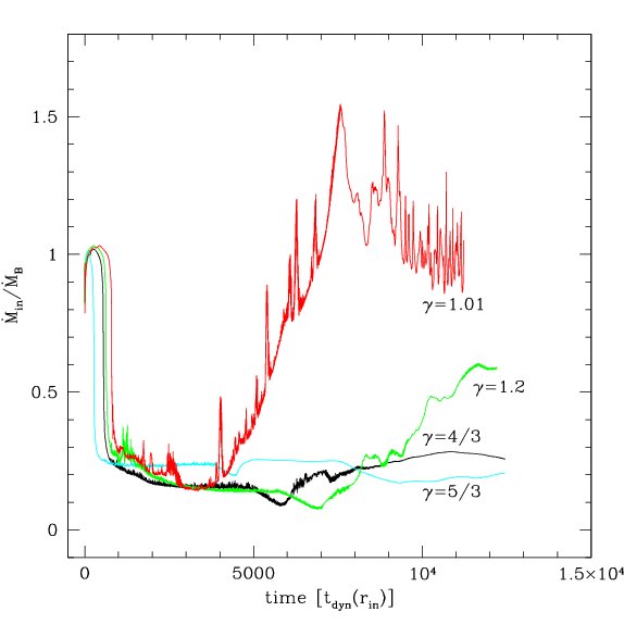
Figure 1: Time evolution of the mass accretion rate through the inner boundary ($\dot{M}_{\rm in}$), in units of the Bondi rate ($\dot{M}_{\rm B}$). The models are: $A$ (red line), $B$ (green line), $C$ (black line), $D$ (cyan line).

In Figure 1 we show the time evolution of the accretion rate through the inner boundary, $\dot{M}_{\rm in}$ (in units of the Bondi accretion rate), for various adiabatic indices. As the Figure shows, the accretion rate onto BH varies in time. Before the rotating material approaches the black hole, $\dot{M}_{\rm in}$ is equal to the Bondi accretion rate for all models. Once the gas starts rotating also in the innermost parts, the accretion rate drops to a small fraction of the Bondi rate. The moment when this happens, i.e. the end of the transient phase of the purely radial accretion, depends on the adiabatic index, and is in the range from about $t^{{}^{\prime}}=3.2\times 10^{2}$ for $\gamma=5/3$, up to about $t^{{}^{\prime}}=9.5\times 10^{2}$ for $\gamma=1.01$.

In all the models, the accretion rate after the torus has formed, is on average low, and does not exceed 30% of the Bondi rate. The fluctuations of the accretion rate for $\gamma=1.2$, 4/3 and 5/3 are not significant: they are on the order of $0.02-0.04\dot{M}_{\rm B}$. However at the end of the simulation, for $\gamma=1.2$ the accretion rate approaches and exceeds $0.5\dot{M}_{\rm B}$. For the almost isothermal model ($\gamma=1.01$), this happens much earlier. The small accretion rate is kept only for a very short time, $t^{{}^{\prime}}\sim 3.9\times 10^{3}$, and after that $\dot{M}_{\rm in}$ starts rising, to reach and exceed the Bondi rate. This is accompanied by very large fluctuations of the accretion rate, in a form of pronounced flares with amplitude of $0.3-0.5\dot{M}_{\rm B}$.

In the Figure 2, we plot the evolution of the angular momentum flux through the inner boundary: $\dot{L}_{\rm in}=\int l_{\rm spec}\rho v_{r}ds$, in units of the critical angular momentum $l_{\rm crit}$ and renormalized by the value of the Bondi accretion rate. At the beginning of the simulation, $\dot{L}_{\rm in}=0$, because in the vicinity of the black hole the gas is not rotating. Once the rotating matter reaches the inner boundary, the angular momentum starts accreting to the center, and $\dot{L}_{\rm in}$ sharply increases. However, after several orbital cycles the outflow begins and the net radial velocity as well as the density near the polar regions drop, so $\dot{L}_{\rm in}$ decreases to a moderate value of $\sim 0.1$ (in the units of $l_{\rm crit}\dot{M}_{\rm B}$). This is the case for the gas and ratiation pressure dominated models, $\gamma=5/3$ and $\gamma=4/3$, and also for the model with $\gamma=1.2$ for most of the simulation. Only for the model with $\gamma=1.01$, the angular momentum flux rises after $t\sim 3.9\times 10^{3}$ and strongly oscillates.

Note that the quantity plotted in the Figure 2 is a flux of total angular momentum, not specific angular momentum. This corresponds to the amount of angular momentum which may be transferred to the black hole and used to spin it up. Figure 2 can be used to calculate the total angular momentum which the black hole could gain during our simulation. We find, after the proper unit conversions, that this number is extremely low: $a=(cJ)/GM^{2}\approx 4\times 10^{-6}-10^{-5}$, where $J=\dot{L}_{\rm in}\Delta t$. For the isothermal model, $\gamma=1.01$, the amount of the total angular momentum accreted onto the black hole will be 2-3 times larger (cf. Fig. 1). Still, it does not lead to the spin-up of the black hole, as the material which is being accreted is the very slowly rotating gas mostly from the polar regions. In the models with $\gamma=5/3,4/3$ and 1.2, the accretion rate and $L_{\rm in}$ are only slightly variable.

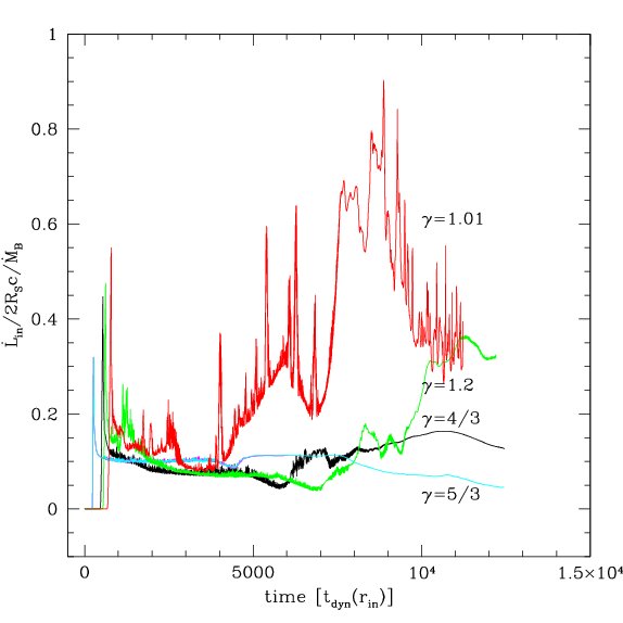
Figure 2: Time evolution of the angular momentum flux through the inner boundary, in units of the critical angular momentum times the Bondi accretion rate. The models are: $A$ (red line), $B$ (green line), $C$ (blackline), $D$ (cyan line).

To understand the behaviour of the accretion rate $\dot{M}_{\rm in}$, we need to study the structure of the flow. In Figures 3, 5, 7 and 9, we plot the contour maps of the density and velocity fields in the innermost regions of the flow (i.e. up to 20 $R_{\rm S}$), for the models A,B,C and D, respectively. The maps are plotted in three time-snapshots, and in the two views: equatorial plane and side-on.

In Figure 3 we show the density contour maps for the inner region of the accretion flow, for the model A ($\gamma=1.01$). The maps also show the velocity field, and are plotted for several snapshots during the evolution: $t^{{}^{\prime}}\approx 3\times 10^{3}$, $t^{{}^{\prime}}\approx 6.3\times 10^{3}$ and $t^{{}^{\prime}}\approx 1.1\times 10^{4}$. The panels on the left, show the side-on view of the inner torus, i.e. the $x-z$-plane, while the panels on the right show the top-view, i.e. the equatorial plane.

The torus, which formed after the transient phase of the Bondi accretion, is very dense: the maximum density in the equatorial plane exceeds $8\times 10^{6}\rho_{\infty}$. At the time $t^{{}^{\prime}}\sim 3\times 10^{3}$, the polar regions are clean, and most of the material is settled near the equator. The radial infall of material onto the central black hole goes mainly through the poles, while the torus material is turbulent and due to the centrifugal barrier the gas may flow outwards. At this time, the rate of accretion through the inner boundary, $\dot{M}_{\rm in}$, is the lowest and is below 20% of the Bondi rate. The rapid variations of the accretion rate are caused by the turbulences. Later, the variations are enhanced by the azimuthal perturbations, which grow in the density field in the innermost region of the torus (see the middle-right panel of the Figure 3, for time $t^{{}^{\prime}}\sim 6.3\times 10^{3}$). As was shown in Figure 1, in the late phase of the evolution in model A, the accretion rate $\dot{M}_{\rm in}$ steeply rises, reaches the Bondi rate, and rapidly varies about this value. However, the flow does not return completely to a spherically symmetric configuration of the Bondi type. The inner torus still exists, but becomes much smaller and its density is lower. The maximum density in the equatorial plane is now about $\sim 2\times 10^{6}\rho_{\infty}$, while the density in the polar regions becomes larger.

Now the polar material forms a kind of streams, in which the density is about 100 times larger in the end of the run than it was during the phase of ’clean poles’. This large density, in addition to the highly supersonic radial velocities (see Fig. 4 below), are the cause for the net accretion rate to be large again. The streams are formed by the material that has too large angular momentum to accrete radially, but flows laminarly over the torus and turns toward the poles. The ’arcs’ visible on the density map are the results of the obligue shocks, where the $v_{\theta}$ velocity component is changing.

We note, that such kind of behaviour, i.e. the drammatic rise of the accretion rate in the nearly isothermal mode, $\gamma=1.01$, was not found in the study by Mościbrodzka & Proga (2008), however, their 2-D runs were performed within twice longer timescale, with $T_{\rm end}\sim 4\times 10^{4}$. In their simulations, a twice smaller rotation parameter was used, $l_{0}=0.05$, so that the accretion rate $\dot{M}_{\rm in}$ in their models did not drop below $\sim 0.4\dot{M}_{\rm B}$. We tested that the difference in the rotation parameter is not crucial: we made the test calculations with other values of $l_{0}$ and qualitatively the results were similar. Also, we checked that it is not the role of the 3-D effects, that make the nearly isothermal torus smaller and weaker after a short time in our simulation. The same model was tested in the 2.5-D axisymmetric configuration with ZEUS-MP, and we found that the mean accretion rate also increased to about $\dot{M}_{\rm B}$ after $t^{{}^{\prime}}\sim 6\times 10^{3}$, with the flaring behaviour being even more pronounced than in our 3-D case.

What we found crucial for the behaviour of the flow at small $\gamma$, was the treatment of the outer boundary condition for the azimuthal velocity. In their simulations with ZEUS 2-D, Mościbrodzka & Proga (2008) imposed the update of specific angular momentum at the outer boundary in every time step. In our simulations, we imposed the rotation of the outer regions only in the initial condition, to mimic the transient cloud of gas, that contains some angular momentum, passing by the vicinity of the galaxy center. When the cloud sinks into the Bondi sphere, the remaining gas at infinity no longer rotates. The Bondi sphere is still modeled with the boundary condition for density, and matched with the analytical Bondi solution.

We note here, that despite the rise of the accretion rate to the value of the Bondi rate, the torus in the innermost parts of the flow does not completely disappear. The torus shrinks in size and is less dense, because of the massive inflow of the non-rotating material from the outer boundary. However, it still acts as an obstacle for the gas flowing radially onto the black hole, which results in the rapid fluctuations of the accretion rate at the inner boundary.

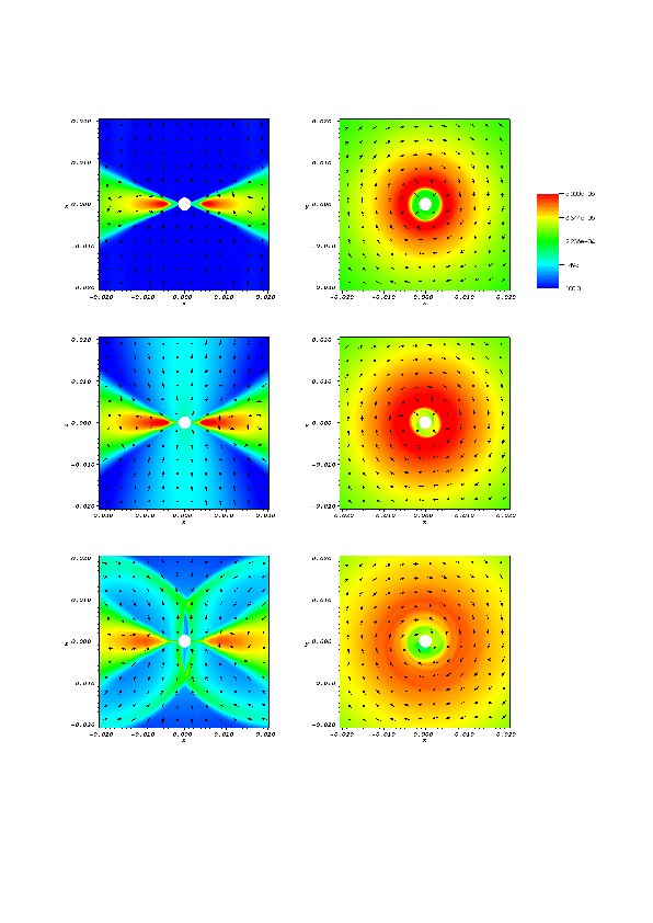
Figure 3: Contour density maps and velocity field in the inner region for the model A ($\gamma=1.01$), in the side-view (along the x-axis; left) and in the top view (along the z-axis; right). The time snapshots are taken at $t^{{}^{\prime}}=3\times 10^{3},6.3\times 10^{3}$ and $1.1\times 10^{4}$, from top to bottom. The units on the x, y and z axes are in $R_{\rm B}$.

In Figure 4 we show the contour plots of the total Mach number, $M_{\rm tot}=|\vec{v}|/c_{\rm s}$ (left) and the radial Mach number, $M_{\rm r}=v_{\rm r}/c_{\rm s}$ (right), for $\gamma=1.01$. The color contours show the constant Mach number of 0.5, 1.0 and 1.5 (red, green and blue, respectively), while the grey colors show the three chosen constant denity contours, to mark the position of the inner torus. In model $A$, which is nearly isothermal, most of the flow is highly supersonic. Starting from the Bondi solution, the sonic radius is located at a very large distance, $r_{\rm s}=0.49R_{\rm B}$, and the total Mach number is everywhere by definition equal to the radial one. When the torus forms, it is supported by rotation, and the radial velocity in the torus is smaller than the sound speed. Only in the innermost radii, below $\sim 2.6\times 10^{-3}R_{\rm B}=2.6R_{\rm S}$, the radial Mach number is greater than 1.0. The sonic radius for the total Mach number is however at the same place as before, and the net velocity of the flow is supersonic. At the time $t^{{}^{\prime}}\sim 6.3\times 10^{3}$ (middle panels of the Figure 4), the sonic radius in the equatorial region shrinks. The radial and the total Mach numbers are both greater than 1.0 close to the poles. The supersonic velocity components closer to the equatorial plane are mostly non-radial. Later during the simulation, this trend reverses. The sonic surface for $M_{\rm tot}$ closes again at $\sim 0.5R_{\rm B}$, and it coincides with the sonic surface for $M_{\rm r}$ (not shown in the bottom-right figure, because of the zooming-in). Close to the equatorial plane, the region with subsonic radial velocities shrinks several times, and at the outer edge of the torus, the radial velocity is equal to the sound speed. What is also worth noticing in Fig. 4, is that the actual size of the constant density contours, that has shrunken about 10 times in the last time snapshot.

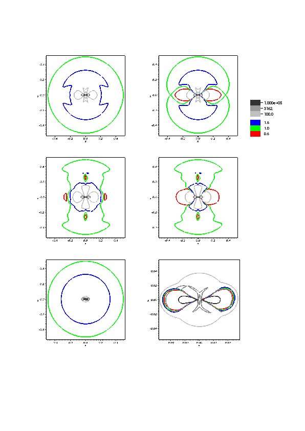
Figure 4: Contour plots of the total Mach number, $M_{\rm tot}$ (left) and the radial Mach number, $M_{\rm r}$ (right) for the model A ($\gamma=1.01$). The time snapshots are taken at $t^{{}^{\prime}}=3\times 10^{3},6.3\times 10^{3}$ and $1.1\times 10^{4}$, from top to bottom. The units on the x and z axes are in $R_{\rm B}$, (the bottom-right panel is zoomed-in). The color contours show the constant Mach number of 0.5, 1.0 and 1.5 (red, green and blue, respectively), while the grey colors show the constant density contours, between $10^{2}$ and $10^{5}\rho_{\infty}$.

In Figure 5 we show the flow topology for the model B ($\gamma=1.2$). In this model, the density of the torus is much lower. Initially, the flow is axially symmetric, but at the time $t^{\prime}\sim 6.3\times 10^{3}$, the axial symmetry is broken. This is because the material at one side of the torus (i.e. the azimuth $\phi\sim 0^{\circ}$), tries to reach the black hole and flows in above the equatorial plane, while at the other side (i.e. the azimuth $\phi\sim 180^{\circ}$), the gas tries to flow in below the equatorial plane. This is shown by the directions of the arrows that represent the velocity field. As was already shown in Janiuk et al. (2008), such a behaviour leads to the tilt of the torus, and here the tilt is clearly visible at the time $t^{\prime}\sim 1.1\times 10^{3}$.

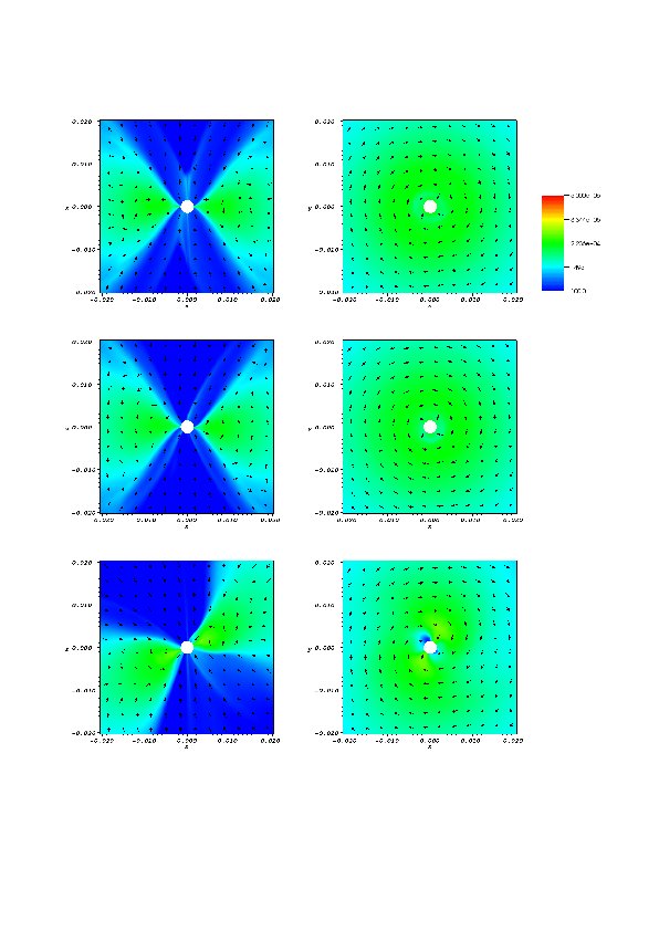
Figure 5: Contour density maps and velocity field in the inner region for the model B ($\gamma=1.2$), in the side-view (along the x-axis; left) and in the top view (along the z-axis; right). The time snapshots are taken at $t^{{}^{\prime}}=3\times 10^{3},6.3\times 10^{3}$ and $1.1\times 10^{4}$, from top to bottom. The units on the x, y and z axes are in $R_{\rm B}$.

In Figure 6 we show the Mach number contours for the model $B$, $\gamma=1.2$. The color contours show the constant Mach number of 0.5, 1.0 and 1.5 (red, green and blue, respectively), while the grey colors show the constant denity contours, to mark the position of the inner torus. The shape of the sonic surface is very different from the previous case (in model A), and resembles in shape the number “eight”. The radial velocity exceeds the speed of sound in the polar regions, while near the equator, somewhat irregular contour of the total Mach number shows the contribution from the supersonic, non-radial velocity components. When the torus gets tilted, the innermost part of the sonic surface tilts as well, and the size of this surface slightly increases.

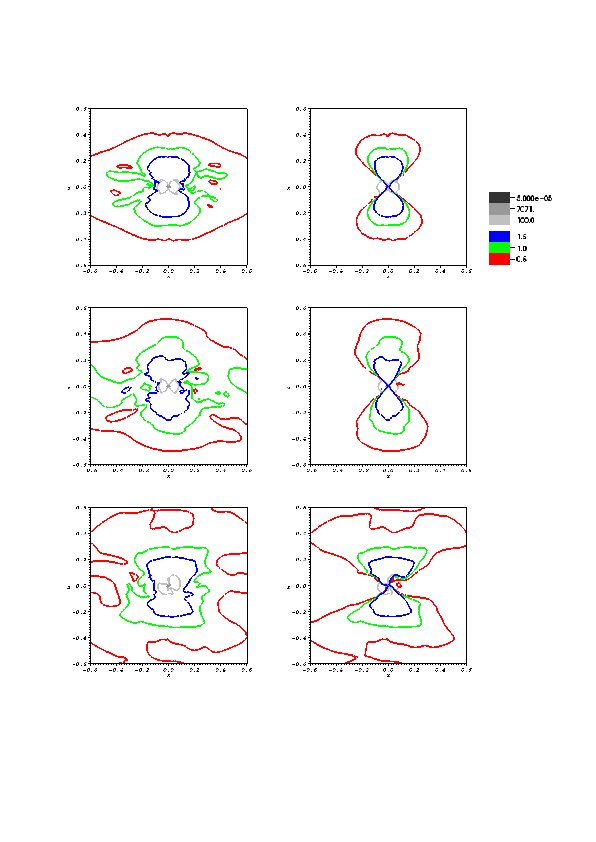
Figure 6: Contour plots of the total Mach number, $M$ (left) and the radial Mach number, $M_{\rm r}$ (right) for the model B ($\gamma=1.2$). The time snapshots are taken at $t^{{}^{\prime}}=3\times 10^{3},6.3\times 10^{3}$ and $1.1\times 10^{4}$, from top to bottom. The units on the x and z axes are in $R_{\rm B}$. The color contours show the constant Mach number of 0.5, 1.0 and 1.5 (red, green and blue, respectively), while the grey colors show the constant denity contours, between $10^{2}$ and $10^{5}\rho_{\infty}$.

Similar results are obtained for the adiabatic indices $\gamma=4/3$ and $\gamma=5/3$. The density maps are shown in Figures 7 and 9, while the Mach number contours are shown in Figures 8 and 10. We note that qualitatively, the basic pattern of the torus evolution is uniform for $\gamma=1.2,4/3$ and 5/3 in the time scale of our simulations. We note that there is a systematic decrease in the torus densities with increasing $\gamma$ (in Fig. 9 the color scale had to be changed to make the density maps more contrasted).

We also note here that in the late time evolution of model $D$, seen in Fig. 9 (bottom-left panel), the flow pattern is strongly affected by the poles. This is the result of a discontinuity at the z-axis, characteristic for the RTP coordinate system. The boundary conditions in the theta direction, which we use in our calculations (reflection with inversion in 2nd and 3rd velocity component), are appropriate as long as the flow is basically axisymmetric. Because in the late time evolution the torus tilts, the z-axis is no longer the symmetry axis. Especially, for the model D the tilt is largest (see below, Sec. 3.2), so the pole effects for this $\gamma=5/3$ are the strongest at the end of the evolution.

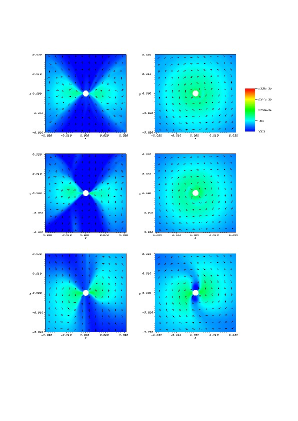
Figure 7: Contour density maps and velocity field in the inner region for the model C ($\gamma=4/3$), in the side-view (along the x-axis; left) and in the top view (along the z-axis; right). The time snapshots are taken at $t^{{}^{\prime}}=3\times 10^{3},6.3\times 10^{3}$ and $1.1\times 10^{4}$, from top to bottom. The units on the x, y and z axes are in $R_{\rm B}$.

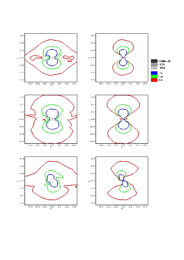
Figure 8: Contour plots of the total Mach number, $M$ (left) and the radial Mach number, $M_{\rm r}$ (right) for the model C ($\gamma=4/3$). The time snapshots are taken at $t^{{}^{\prime}}=3\times 10^{3},6.3\times 10^{3}$ and $1.1\times 10^{4}$, from top to bottom. The units on the x and z axes are in $R_{\rm B}$. The color contours show the constant Mach number of 0.5, 1.0 and 1.5 (red, green and blue, respectively), while the grey colors show the constant denity contours, between $10^{2}$ and $10^{5}\rho_{\infty}$.

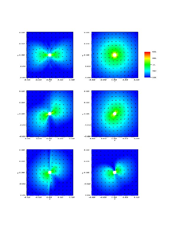
Figure 9: Contour density maps and velocity field in the inner region for the model D ($\gamma=5/3$), in the side-view (along the x-axis; left) and in the top view (along the z-axis; right). The time snapshots are taken at $t^{{}^{\prime}}=3\times 10^{3},6.3\times 10^{3}$ and $1.1\times 10^{4}$, from top to bottom. The units on the x, y and z axes are in $R_{\rm B}$.

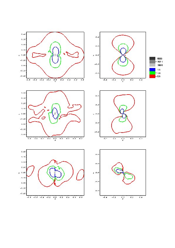
Figure 10: Contour plots of the total Mach number, $M$ (left) and the radial Mach number, $M_{\rm r}$ (right) for the model D ($\gamma=5/3$). The time snapshots are taken at $t^{{}^{\prime}}=3\times 10^{3},6.3\times 10^{3}$ and $1.1\times 10^{4}$, from top to bottom. The units on the x and z axes are in $R_{\rm B}$. The color contours show the constant Mach number of 0.5, 1.0 and 1.5 (red, green and blue, respectively), while the grey colors show the constant denity contours, between $10^{2}$ and $10^{5}\rho_{\infty}$.

To summarize and compare the evolution of the flow for various adiabatic indices, we show the large scale poloidal velocity fields, plotted for models A,B,C and D, at three representative time snapshots. Figure 11 shows, from top to bottom, the velocity fields at time $t^{{}^{\prime}}=3\times 10^{3},6.3\times 10^{3}$ and $1.1\times 10^{4}$, taken at the azimuth $\phi=0$. Because the model is not axially symmetric, the snapshots taken at different azimuths will not look exactly the same. Nevertheless, the global pattern, which depends mainly on $\gamma$, is very similar. The first column shows the model with $\gamma=1.01$. Here, the torus which formed initially in the equatorial region, is accompanied by the departure of the velocity field from the purely radial. The gas turns back due to the centrifugal force, however no net outflow occurs, and the largest size of the turbulent region is about 200 $R_{\rm Schw}$. In the last time snapshot, for $\gamma=1.01$ the torus is indeed very small, and the size of the turbulent region is only about 20 $R_{\rm Schw}$, hardly visible in the scale of the Figure.

For other models, the turbulent region is much larger, and grows with $\gamma$. The shock front between the outflowing and inflowing gas is clearly visible, and this front propagates outwards with time. The large outflow of material occurs from the equatorial region, and is accompanied by the large scale turbulences.

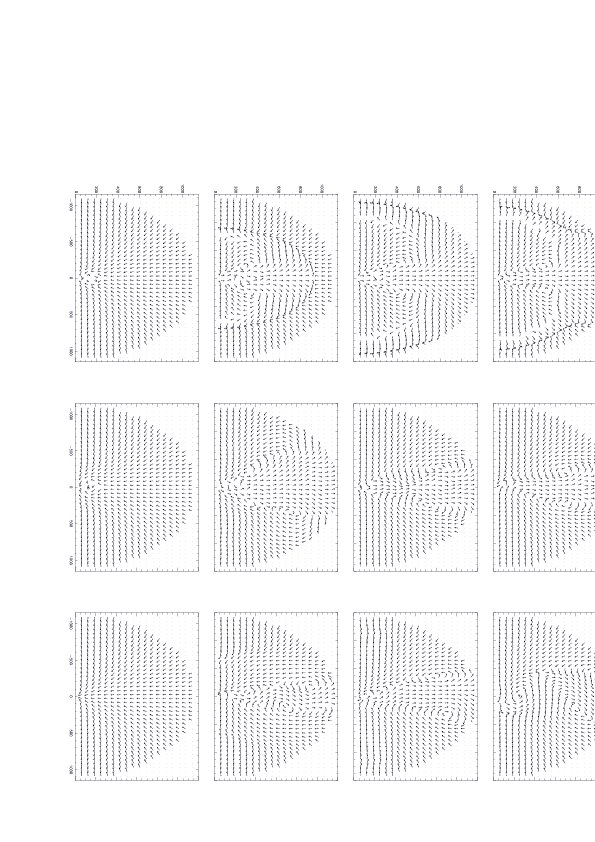
Figure 11: Sequences of the poloidal velocity fields, taken for the azimuth $\phi=0$, for the models with $\gamma=1.01,1.2,4/3$ and 5/3 (from left to right) and at three different time snapshots: $t^{{}^{\prime}}=3\times 10^{3},6.3\times 10^{3}$ and $1.1\times 10^{4}$ (from top to bottom).

3.2 Torus precession

The precession of the torus is discussed below in terms of the tilt and twist angles. These angles are defined as (see e.g. Fragile et al. 2007; Janiuk et al. 2008):

$$\beta(r,t)=\arccos\Big{(}{L_{z}\over L}\Big{)}$$ (18)

and

$$\gamma(r,t)=\arccos\Big{(}{L_{x}\over\sqrt{L_{x}^{2}+L_{y}^{2}}}\Big{)}.$$ (19)

Initially, the flow is axisymmetric and the only component of the angular momentum vector is $L_{\rm z}$ (which sign depends on the direction of the flow rotation), while $L_{\rm x}$ and $L_{\rm y}$ are basically zero. Therefore the tilt angle is vanishingly small and the disk does not precess. After some time, the non-zero $L_{\rm x}$ and $L_{\rm y}$ components appear in the flow, while $|L_{\rm z}|$ decreases, and the rotation axis tilts towards the $x-y$ plane. Then, $L_{\rm y}$ and $L_{\rm x}$ are changing periodically, with $L_{\rm z}$ being almost constant, i.e. the rotation axis moves clockwise or counter-clockwise, depending on the model.

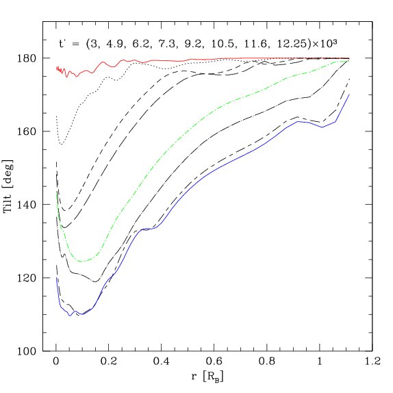
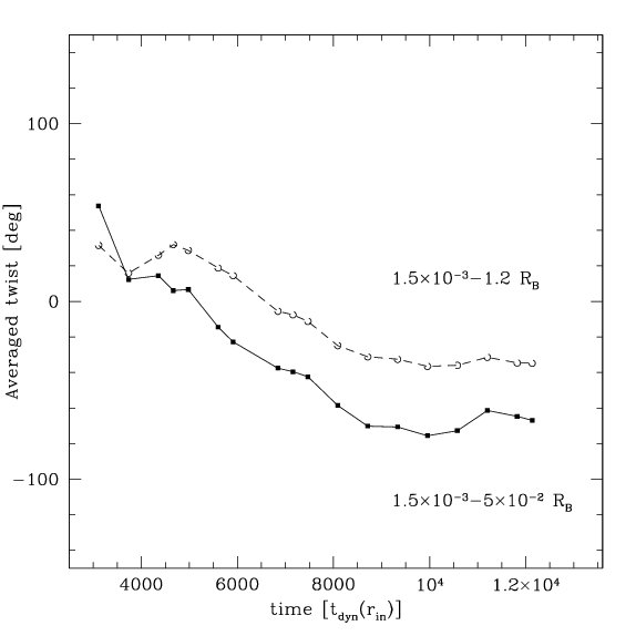
Figure 12: The tilt (left panel) and averaged twist (right panel) angles, calculated for model with $\gamma=5/3$. The tilt is shown as a function of radius, for several time-snapshots, given in the top of the panel. The initial tilt is of 180^∘, meaning that the angular momentum vector is not tilted to the z-axis and the flow rotates with a negative azimuthal velocity. The twist angle is shown as a function of time, and the two curves represent the averaging over radius from $r=r_{\rm in}$ to $r=0.05R_{\rm B}$ (solid line) and to $r=1.2R_{\rm B}$ (dashed line). The twist angle decreasing from $\sim 60^{\circ}$ to $\sim-80^{\circ}$ (innermost torus) and from $\sim 40^{\circ}$ to $\sim-40^{\circ}$ (total) reflects the clockwise, initially differential precession.

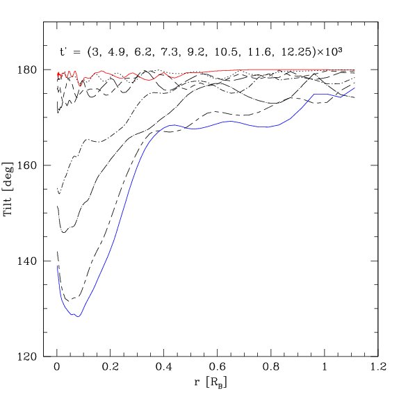
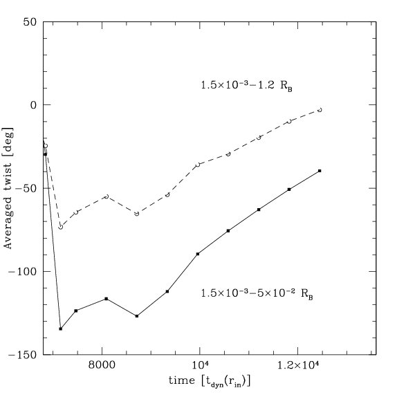
Figure 13: The tilt (left panel) and averaged twist (right panel) angles, calculated for the model with $\gamma=4/3$. The tilt is shown as a function of radius, for several time-snapshots, given in the top of the panel. The initial tilt is of 180^∘ means that the angular momentum vector is not tilted to the z-axis and the flow rotates with a negative azimuthal velocity. The twist angle is shown as a function of time, and the two curves represent the averaging over radius from $r=r_{\rm in}$ to $r=0.05R_{\rm B}$ (solid line) and to $r=1.2R_{\rm B}$ (dashed line). The twist angle increasing from $\sim-120^{\circ}$ to $\sim-40^{\circ}$ (innermost torus) and from $\sim-70^{\circ}$ to $\sim 0^{\circ}$ (total) reflects the counter-clockwise, initially differential precession.

The evolution of the tilt and twist angles proceeds as follows. The tilt (i.e. the angle between the angular momentum vector of the gas and the $z$ axis), is initially equal to zero for all radii. Later during the simulation the tilt rises strongly in the inner parts of the flow, while it is negligible in the outer parts. The twist angle is defined as a cumulative angle by which the angular momentum vector revolves in the $x-y$ plane by the time $t$. Before the disk was tilted, it did not precess, and by definition the twist was zero everywhere. When the tilt increases, the twist angle rises fast in the innermost parts of the flow, which we show in the Figure 12 (as well as in the following Figures 13, 14 and 15) as the twist averaged over the radius, from $r_{\rm in}$ to $0.05R_{\rm B}$. Initially, the strongest rise for the innermost radii implies the differential precession of the torus. The outermost parts of the flow have a negligible precession, and above $\sim 0.5R_{\rm B}$ the twist oscillates around zero. The total twist, i.e. the average over the radius from $r_{\rm in}$ to $r_{\rm out}$, is smaller than that for the innermost torus.

In the Figure 12 we show the tilt and twist evolution for the model with $\gamma=5/3$. The tilt is shown as a function of radius, for several time-snapshots. The initial tilt of 180^∘ means that the angular momentum vector is not tilted and the flow rotates with a negative azimuthal velocity. The twist angle is shown as a function of time, and the averaging over radius was calculated in two ranges: from $r=r_{\rm in}$ to $r=0.05R_{\rm B}$ (solid line) and to $r=1.2R_{\rm B}$ (dashed line). The twist angle decreasing from $\sim 60^{\circ}$ to $\sim-80^{\circ}$ (innermost torus) as well as from $\sim 40^{\circ}$ to $\sim-40^{\circ}$ (total) reflects the clockwise precession. Initially, the precession is differential, i.e. only the innermost parts of the torus tilt and twist. Later, during the time evolution, also the outer parts of the flow tilt, and the last two time snapshots in the left panel of the Figure 12 show that the tilt increases uniformly for all radii. In the right panel of the same Figure, the slopes of the dashed and solid lines at late times are nearly the same, meaning that after the period of a differential precession, the torus is precessing as a nearly solid body.

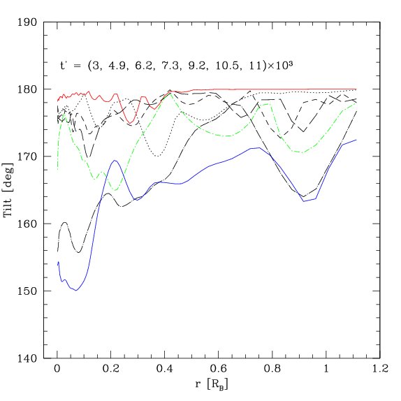
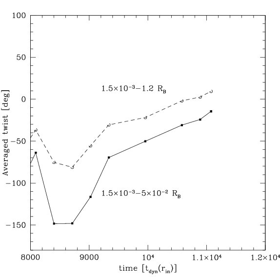
Figure 14: The tilt (left panel) and averaged twist (right panel) angles, calculated for the model with $\gamma=1.2$. The tilt is shown as a function of radius, for several time-snapshots, given in the top of the panel. The initial tilt is of 180^∘ means that the angular momentum vector is not tilted to the z-axis and the flow rotates with a negative azimuthal velocity. The twist angle is shown as a function of time, and the two curves represent the averaging over radius from $r=r_{\rm in}$ to $r=0.05R_{\rm B}$ (solid line) and to $r=1.2R_{\rm B}$ (dashed line). The twist angle increasing from $\sim-150^{\circ}$ to $\sim-10^{\circ}$ (innermost torus) and from $\sim-80^{\circ}$ to $\sim 10^{\circ}$ (total) reflects the counter-clockwise, initially differential precession.

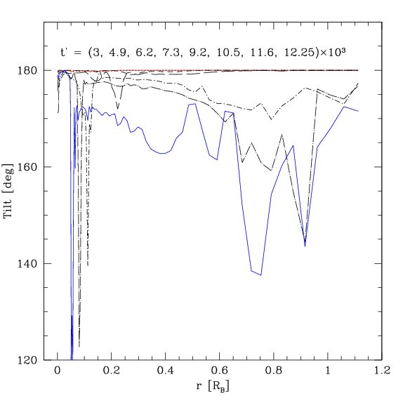
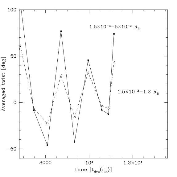
Figure 15: The tilt (left panel) and averaged twist (right panel) angles, calculated from the time evolution of the model $A$ ($\gamma=1.01$). The tilt is shown as a function of radius, for several time-snapshots, given in the top of the panel. The initial tilt is of 180^∘ means that the angular momentum vector is not tilted and the flow rotates with a negative azimuthal velocity. The twist angle is shown as a function of time, and the two curves represent the averaging over radius from $r=r_{\rm in}$ to $r=0.05R_{\rm B}$ (solid line) and to $r=1.2R_{\rm B}$ (dashed line). The angular momentum vector is always almost perpendicular to the equatorial plane, and despite the large scatter in the two angles, the apparent small tilt is due to the very small components of $L_{\rm x}$ and $L_{\rm y}$.

In Figure 13 we plot the tilt and twist angles for the model with $\gamma=4/3$. Here again, the initial tilt is of 180^∘, meaning no tilt and negative azimuthal velocity. The twist angle increasing from $\sim-120^{\circ}$ to $\sim-40^{\circ}$ (innermost torus) as well as from $\sim-70^{\circ}$ to $\sim 0^{\circ}$ (total) shows the counter-clockwise, initially differential, and at late times a nearly solid body precession.

In Figure 14 we plot the tilt and twist evolution for $\gamma=1.2$. The precession starts even later than in case of $\gamma=4/3$, and proceeds also counter-clockwise.

For the model with $\gamma=1.01$, we cannot confirm neither tilt no precession of the torus. In Figure 15, there is no trend of increase for the tilt and twist angles, and the large scatter in the two angles is caused by the virtually very small components of the angular momentum vector, $L_{\rm x}$ and $L_{\rm y}$. We find that the tilt fluctuates periodically and no clear signs of precession towards any direction can be detected.

We estimated the times when precession started, and periods of precession, for models B,C and D. The start times are: $t^{{}^{\prime}}=4\times 10^{3}$, $8.5\times 10^{3}$ and $9.5\times 10^{3}$, for $\gamma=5/3,4/3$ and 1.2, respectively. The delays in the torus tilt are corresponding to the similar delays in the torus formation, in case of smaller $\gamma$ with respect to $\gamma=5/3$. On the other hand, the precession period can be estimated at $2.4\times 10^{4}$, $1.6\times 10^{4}$ and $6.4\times 10^{3}$. Therefore we conclude, that the larger the adiabatic index, the earlier the torus forms and starts precessing, while the longer the precession period.

For $\gamma=1.01$ no such estimates could be made, because the torus shrank too much before it could start precessing. However, we note that on the density map (Fig. 3, middle right panel) there is a non-axisymmetric structure, which develops in the innermost region. This might be a hint for an azimuthal ($m=2$) instablity mode that starts developing at this time in the simulations. Therefore we made an additional test calculation, model $Av$, in which we changed the outer boundary condition for the velocity and we continuously added the angular momentum at the outer radius. In this way, the torus could be supported rotationally for a very long time during the simulation, and did not shrink like in model $A$.

The accretion rate dependence on time for this model is shown in Figure 16. There is clearly no rapid rise of the accretion rate above the Bondi value, and the mean accretion rate is rather small, $0.3\dot{M}_{\rm B}$. The rapid and large fluctuations of the accretion rate appear however, and temporarily the accretion rate flare can reach even 0.75 of the Bondi rate. These changes are are caused by the oscillations at the outer edge of the torus, similarly to those found in Mościbrodzka & Proga (2008) in their 2-dimensional computations, however in our 3D case the amplitude of these oscillations is much larger.

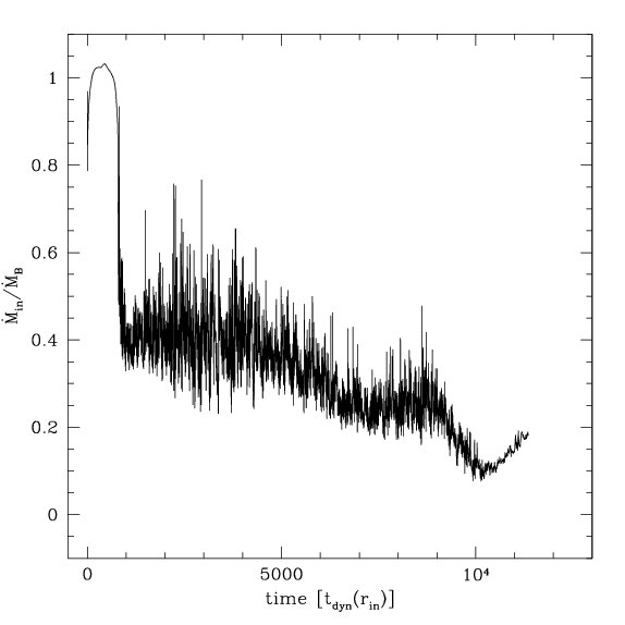
Figure 16: Time evolution of the mass accretion rate through the inner boundary ($\dot{M}_{\rm in}$), in units of the Bondi rate ($\dot{M}_{\rm B}$). The model is $Av$, i.e. $\gamma=1.01$ but with the changed outer boundary condition.

In Figure 17 we plot the tilt and twist angles for the model $Av$. The initial tilt is 0^∘, because the flow rotated initially with a positive azimuthal velocity. Than, the tilt increased, mostly in the innermost radii, and in the end of our simulation it reached $40^{\circ}$ at 0.2 $R_{\rm B}$. The tilt is initially differential, and smoothly decreases with radius. The tilt angle for the innermost part, i.e. averaged from $r=r_{\rm in}$ to $r=0.05R_{\rm B}$, initially was periodically changing. Despite large values of the tilt, it was due to the very small components of $L_{\rm x}$ and $L_{\rm y}$. After time $t^{\prime}>10^{4}$, the torus started precession, and the twist angle decreased from $\sim 20^{\circ}$ to $\sim-20^{\circ}$ (innermost torus) and from $\sim 0^{\circ}$ to $\sim-30^{\circ}$ (total). We estimated that the precession period is below $\sim 6.3\times 10^{3}$, and the precession started from $t^{\prime}=1.05\times 10^{4}$. Therefore the trend of the tilt moment decreasing and the precession period increasing with $\gamma$ is confirmed also for $\gamma=1.01$, if the torus is supported by the constant inflow of the rotating material from the outer boundary.

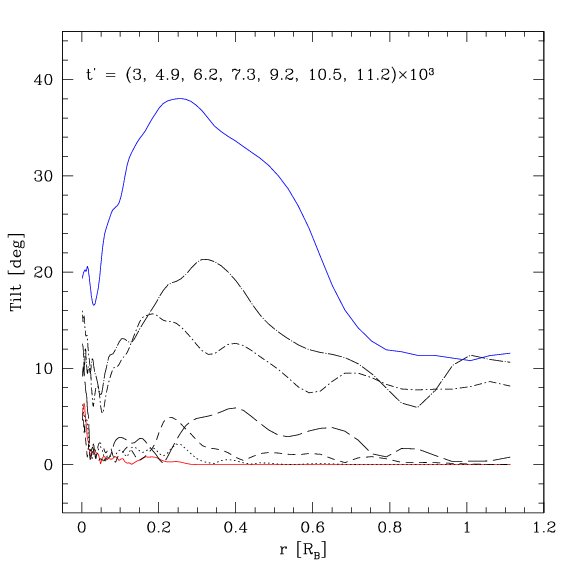
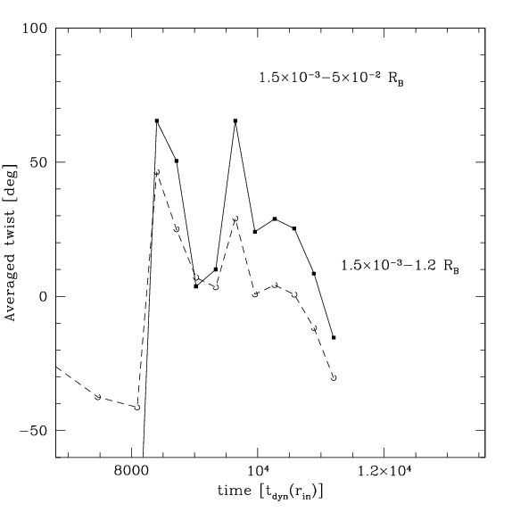
Figure 17: The tilt (left panel) and averaged twist (right panel) angles, calculated from the time evolution of the model $Av$ ($\gamma=1.01$, but with the changed outer boundary condition). The tilt is shown as a function of radius, for several time-snapshots, given in the top of the panel. The initial tilt of 0^∘ means that the angular momentum vector is not tilted and the flow rotates with a positive azimuthal velocity. The twist angle is shown as a function of time, and the two curves represent the averaging over radius from $r=r_{\rm in}$ to $r=0.05R_{\rm B}$ (solid line) and to $r=1.2R_{\rm B}$ (dashed line). The twist angle decreasing from $\sim 20^{\circ}$ to $\sim-20^{\circ}$ (innermost torus) and from $\sim 0^{\circ}$ to $\sim-30^{\circ}$ (total) reflects the clockwise, initially differential precession, starting from time $t^{\prime}>10^{4}$.

3.3 Evolution of the flow for various gas temperatures

We calculated the models with various positions of the Bondi radius with respect to the Schwarzschild radius, which is reflected by a different sound speed at infinity and gas temperature. In the models with smaller $R_{\rm B}/R_{\rm S}$, the evolution proceeds faster and the torus forms much earlier: at $t^{{}^{\prime}}=4\times 10^{2}$ for $R_{\rm B}/R_{\rm S}=300$ and at $t^{{}^{\prime}}=2\times 10^{2}$ for $R_{\rm B}/R_{\rm S}=100$.

During the torus evolution, in these models we detect neither tilt nor precession. The accretion rate onto the black hole is much below the Bondi rate and it is fluctuating (Figure 18). These oscillations are caused by a strong outflow of material that occurs periodically because the gas wants to remove some angular momentum (note that the $l_{0}$ parameter, i.e. the circularisation radius, is the same in all models).

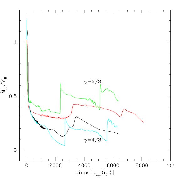
Figure 18: Time evolution of the mass accretion rate through the inner boundary ($\dot{M}_{\rm in}$), in units of the Bondi rate ($\dot{M}_{\rm B}$). The models are: $E$ (red line), $F$ (green line), $G$ (black line) and $H$ (cyan line). The models have the adiabatic index of $\gamma=5/3$ and $\gamma=4/3$, as labelled on the plot, and temperature determined by the ratio of $R^{\prime}=R_{\rm B}=R_{\rm S}$ is equal to 100 or 300.

Nevertheless, the outflows occur symmetrically in these models, and in the end of the simulation there are no systematic asymmetries with respect to the equatorial plane nor the azimuth. Therefore for the models with large sound speed at infinity, the outflow stabilizes the system with respect to the azimuthal perturbations and there is no precession. The exemplary maps of the velocity field at the end of the simulation for the models $E$, $F$, $G$ and $H$, are shown in Figure 19.

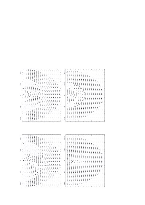
Figure 19: The poloidal velocity field for the $\phi=0$ slice, at the end of the simulation. The models are: $E$ (top left), $F$ (top right), $G$ (bottom left) and $H$ (bottom right).

4 Discussion

In this work, we considered the hydrodynamical models of slightly rotating, non-axisymmetric accretion flows. We studied the role of adiabatic indices, and we verified the results from our previous work considering the precession of the inner torus.

We found that the tilt and precession occur not only for the gas pressure dominated flow, described with the equation of state with $\gamma=5/3$, but also for the radiation dominated gas, modeled with $\gamma=4/3$, as wll as for smaller $\gamma=1.2$. The moment, when the torus gets tilted and starts precessing, correlates with $\gamma$. The period of precession also depends on the adiabatic index, and is shorter for smaller $\gamma$.

We tested also the nearly isothermal gas, with $\gamma=1.01$. In this case, we could not confirm whether the torus precesses, in the model when there is no further angular momentum supply from the outer boundary, except for the initial condition. For small $\gamma$, the torus is very dense and compact, and its evolution is determined by the large scale behaviour of the flow. If the angular momentum is added during the simulation to the outer boundary of the simulation domain, such a torus may survive and keep the accretion rate onto black hole constantly smaller than the Bondi rate. Otherwise, there is a lot of material that quickly falls radially onto the center, and because the speed of sound is very small, most of this material falls in supersonically. The torus shrinks substantially, and the net accretion rate onto the black hole is again on the order of the Bondi rate. The accretion rate fluctuates about this value very rapidly, because the shrunken torus still provides an obstacle for the radially infalling gas. The boundary condition that we used for most of the models in this work, made such a scenario of the flow evolution proceed very fast for small $\gamma$, and much slower for larger $\gamma$.

The net outflow of material from the equatorial plane is not observed in the model with $\gamma=1.01$, and at large scales the flow is spherically symmetric (cf. Mościbrodzka & Proga 2008). However some tilt is visible in the innermost region, it is twice smaller than for $\gamma=5/3$ or $\gamma=4/3$. The twist angle is negligibly small, as both the $L_{\rm x}$ and $L_{\rm y}$ components of the angular momentum vector are tiny. This angle fluctuates periodically, showing no clear signs of precession towards any direction.

However, if the angular momentum is constantly added at the outer boundary, the torus remains large and does not shrink. In such a model, the tilt angle increases after $t^{\prime}>10^{4}$ (units of dynamical times at the inner radius), and the torus starts precessing. Therefore, we conclude that the non-axisymmetric perturbations occur for all types of the equation of state and only the moment when instability starts growing depends on $\gamma$. If for small $\gamma$ the amount of inflow of the rotating material is not sufficient, the torus may shrink before the effects of precession can be observed.

The present work is a follow-up of Janiuk et al. (2008), where we first identified the precession of a torus, developing in the 3-D model of a slowly rotating accretion flow. We found, that if a sufficient amount of angular momentum is added to the initially spherically accreting Bondi flow, the instabilities rise in the innermost gas. The initial perturbations appear due to some small asymmetries in the angular momentum distribution, which in the calculations can be of numerical origins, but to which any physical system is subject. The flow then enters a transient phase of growing acoustic oscillations, which manifest themselves in the fluctuating sonic surface. Subsequently, the transition to a progressive departure from the initial state takes place (i.e. the growing tilt of the inner torus and its precession about the vertical axis).

In Janiuk et al. (2008), as well as in the present work, we checked that the instability develops in a highly supersonic flow, whereas for small Mach numbers it is suppressed. We can attribute this behaviour with the Papaloizou & Pringle (1985) type of instability, which for low order modes is driven by the Kelvin-Helmholtz mechanism. However here, the picture is more complicated due to the supersonic nature of the flow, presence of outflows and shocks, as well as compressibility. The present work was devoted to the effect of the various adiabatic index $\gamma$.

We found that the inner torus precesses also for values other than $\gamma=5/3$, used in our first study: $\gamma=4/3,1.2$, and 1.01. However, the time for the precession to set increases with decreasing $\gamma$. For the nearly isothermal model, $\gamma=1.01$, the time of the instability growth was too long to set the precession, unless the outer boundary condition was changed and more angular momentum was supplied during the time evolution. Our results are in agreement with the general behaviour of the unstable accreting flows for various equations of state. Blondin et al. (2003) studied the stability of standing accretion shocks, and also found that the softer the equation of state (smaller $\gamma$), the slower is the growth of SAS instability. For the smallest $\gamma=1.25$ used by these authors, they found that the shock remained marginally stable for a long period of time, however also this model eventually became as unstable as the others. The physical mechanism that is lying behind this SASI instability is the vortical-acoustic feedback between the pressure waves and vorticities induced by the aspherical shock. Such feedback was also studied by Foglizzo (2002) in the context of accreting black holes. In our simulations, shocks arise due to the outflow of gas in the equatorial plane, and no polar outflows are produced without the magnetic field (see e.g. Mościbrodzka & Proga 2009), but the mechanism appears to be similar.

The mechanism of precession that we present in this work appears to be an additional one, apart from those discussed in the litearture. Caproni et al. (2006) discuss several different sources of the accretion disk warping and precession. It may occur due to the tidal forces, irradiation, magnetically driven instability, or the Bardeen-Petterson effect. Signatures of the disk precession are observed in both AGN and stellar mass black hole or neutron star binaries. The observations involve the spectral and temporal variability as well as the distortions of jet morphology. The period of precession can be quite short, and for the sources with black hole mass on the order of $10^{7}-10^{8}M_{\odot}$ the observed times are on the order of 1-10 years. Our results are in good agreement with these observations of AGN.

To study the precession mechanism in more detail we need to include the magnetic fields in our modeling. If the Kelvin-Helmholtz mechanism lies behind the torus precession instability, the results should be affected by the presence of magnetic field component only in the streaming direction. This is planned to be the subject of our future work. In addition, it will be useful to compare the results of the present ZEUS-MP code with another MHD code available for testing, to help clarify whether the main instability in our studies is of a physical or numerical nature.

References

- (1) Bondi H., 1952, MNRAS, 112, 195
- (2) Blondin J.M., Mezzacappa A., DeMarino C., 2003, ApJ, 584, 971
- (3) Caproni A., Livio M., Abraham Z., Mosquera Cuesta H.J., ApJ, 2006, 653, 112
- (4) Catlett C. et al. ”TeraGrid: Analysis of Organization, System Architecture, and Middleware Enabling New Types of Applications,” HPC and Grids in Action, Ed. Lucio Grandinetti, IOS Press ’Advances in Parallel Computing’ series, Amsterdam, 2007
- (5) Foglizzo T., 2002, A&A, 392, 353
- (6) Fragile P.C., Blaes O.M., Annios P., Salmonson J.D., 2007, ApJ, 668, 417
- (7) Hayes J.C., Norman M.L., 2003, ApJS, 147, 197
- (8) Janiuk A., Proga D., Kurosawa R., 2008, ApJ, 681, 58
- (9) Mościbrodzka M., Proga D., 2008, ApJ, 679, 626
- (10) Mościbrodzka M., Proga D., 2009, MNRAS, 397, 208
- (11) Paczyński B., Wiita P.J., 1980, A&A, 88, 23
- (12) Papaloizou J.C.B., Pringle J.E., 1985, MNRAS, 213, 799
- (13) Proga D., Begelman M., 2003a, ApJ, 582, 69 (PB03)
- (14) Proga D., Begelman M., 2003b, ApJ, 592, 767
- (15) Stone J.M., Norman M.L., 1992, ApJS, 80, 753