Spectroscopic data for the LiH molecule from pseudopotential quantum Monte Carlo calculations

Abstract

Quantum Monte Carlo and quantum chemistry techniques are used to investigate pseudopotential models of the lithium hydride (LiH) molecule. Interatomic potentials are calculated and tested by comparing with the experimental spectroscopic constants and well depth. Two recently-developed pseudopotentials are tested, and the effects of introducing a Li core polarization potential are investigated. The calculations are sufficiently accurate to isolate the errors from the pseudopotentials and core polarization potential. Core-valence correlation and core relaxation are found to be important in determining the interatomic potential.

I introduction

Pseudopotentials are often generated using data from mean-field theories such as density-functional theory and Hartree-Fock (HF) theory, but they are often used in more accurate many-body approaches, such as Multi-Configuration Self-Consistent Field (MCSCF) and quantum Monte Carlo (QMC) calculations. In this paper we apply such methods to a simple system, the LiH molecule with pseudopotentials representing the Li⁺ and H⁺ ions, for which we can obtain very accurate ground state energies. Our main aim is to investigate the accuracy of pseudopotentials for this system, including the performance of a Li core-polarization potential (CPP) which introduces some of the effects of core-valence correlation and core relaxation. The accuracy of the LiH interatomic potentials is measured by calculating the spectroscopic constants of the diatomic molecule and the well-depth, which can readily be compared with experiment. Note that our goal is not to achieve the most accurate ab initio spectroscopic constants - if it were we would solve the all-electron system directly using QMC, or one of the range of accurate methods tractable for a four electron system - but to separate the deficiencies of a model valence Hamiltonian from those of the methods available for its solution.

Our most accurate results are obtained with the variational quantum Monte Carlo (VMC) method and the more sophisticated diffusion quantum Monte Carlo (DMC) method.foulkes_2001 Although the scaling of the computational cost of these calculations with particle number $N$ is reasonable ($\sim$$N^{3}$foulkes_2001 ), the cost increases rapidly with $Z$ ($\sim$$Z^{5.5}$ma05 ; ceperley86 ). It is therefore normal to use pseudopotentials for heavier atoms. It is highly advantageous to use pseudopotentials which are smooth at the origin in VMC and DMC calculations, but most of the pseudopotentials found in the quantum chemistry literature diverge at the origin. We have tested two sets of recently published pseudopotentialstrail05a ; trail05b ; burkatzki07 for the Li⁺ and H⁺ ions, which are smooth at the origin and have been designed for use in QMC calculations. One of these is a “shape-consistent” pseudopotentialtrail05a ; trail05b generated from the Hartree-Fock atomic ground state while the other is an “energy-consistent” pseudopotentialburkatzki07 generated from the ground and excited state energies of the Hartree-Fock atom.

The pseudopotential model of the LiH diatomic molecule contains two valence electrons of opposite spin. The ground state wave function is therefore nodeless, so that no error arises from the “fixed-node approximation” used to enforce the fermion antisymmetry in DMC. However, the DMC energy is not exact, even in principle, because the non-local pseudopotential is treated approximately, although we demonstrate that the error must be small in this case. Our calculations are therefore exacting tests of the accuracy of the pseudopotentials and CPP.

Throughout we consider the error of the LiH diatomic molecule with both Li and H described by pseudopotentials. No attempt is made to separate the performance of each pseudopotential, but atomic calculations suggest that errors arising from deficiencies of the H pseudopotential will be an order of magnitude smaller than those from the Li pseudopotential.

The quality of a diatomic potential can be characterised by the spectroscopic constants, or Dunham coefficients,dunham32 which can be determined experimentally from the rotation/vibration spectrum. Calculations which include an accurate description of electron correlation are computationally expensive and so they are normally performed at a small number of geometries and the interatomic potential is obtained by fitting to a suitable functional form. Fitting to a small number of energies introduces an error which is further exacerbated if the energies have a statistical uncertainty, as in QMC estimates. We explore this problem carefully and ensure that such errors are small. In what follows only the $X^{1}\Sigma^{+}$ (ground) state of the ⁷Li¹H isotopologue is considered.

II spectroscopic constants

A Born-Oppenheimer decoupling of the electron/nucleus coordinates of a diatomic molecule leads to the energy levels

$$E_{vK}=\sum_{ij}Y_{ij}(v+1/2)^{i}K^{j}(K+1)^{j},$$ (1)

where $v$ and $K$ are the vibrational and rotational quantum numbers, and the spectroscopic constants, $Y_{ij}$, depend on the underlying interatomic potential.dunham32 Not all of these coefficients may be extracted directly from experimental data - $Y_{00}$ cannot since it does not influence the spacing of levels, although it is required to define the zero point energy $E_{\rm ZP}=E_{00}$. We follow Dunham and express $Y_{00}$ as

$$Y_{00}=\frac{Y_{01}}{4}-\frac{Y_{11}Y_{10}}{12Y_{01}}+\frac{Y_{11}^{2}Y_{10}^{2}}{144Y_{01}^{3}}+\frac{Y_{20}}{4}+\ldots$$ (2)

for experimental data, while $Y_{00}$ is available directly from ab initio data.

The zero point energy is given by

$$E_{\rm ZP}=Y_{00}+\frac{1}{2}Y_{10}+\frac{1}{4}Y_{20}+\frac{1}{8}Y_{30}+\frac{1}{16}Y_{40}+\ldots,$$ (3)

and the ‘harmonic equilibrium separation’, $R_{e}$, is defined as

$$R_{e}^{2}=\frac{1}{2\mu}\frac{1}{Y_{01}},$$ (4)

where $\mu$ is the reduced nuclear mass of the system, and all quantities are in atomic units. Finally, we note that the spectroscopic constants are normally defined as

$$w_{e} = Y_{10}$$

$$w_{e}x = -Y_{20}$$

$$w_{e}y = Y_{30}$$

$$B_{e} = Y_{01}$$

$$\alpha_{e} = -Y_{11},$$ (5)

although we use the $Y_{ij}$ notation throughout.

To obtain estimates of $\{Y_{ij}\}$ from a set of total energy values requires some further analysis. We fit a highly flexible form for the interatomic potential to a finite number of total energies evaluated at different geometries. We use the “modified Lennard-Jones oscillator”coxon04 ; modpot_extra potential,

$$U(R)=U_{\infty}-D_{e}+D_{e}\left[1-\left(\frac{R_{0}}{R}\right)^{6}e^{-\phi(z)z}\right],$$ (6)

where $U(R)$ is the total energy for interatomic spacing $R$, $R_{0}$ is the position of the minimum in the interaction potential, $D_{e}$ is the well depth, $U_{\infty}$ is the large $R$ limit of $U(R)$, and $\phi(z)$ is defined by

$$\phi(z)=\sum_{m=0}^{M}a_{m}z^{m}$$ (7)

for some choice of $M$, where

$$z=2\frac{(R-R_{0})}{(R+R_{0})}.$$ (8)

A non-linear least-squares fit to $U(R)$ (with $U_{\infty}$ provided by isolated atom calculations using the same method as the diatomic calculations) provides the parameters $(\{a_{m}\},D_{e},R_{0})$. Note that the bond dissociation energy, $D_{0}$, is related to the well depth and the zero point energy by $D_{e}=D_{0}+E_{\rm ZP}$. The derivatives of $U(R)$ at $R_{0}$ may be evaluated and used together with Dunham’s formulaedunham32 to obtain the spectroscopic constants and the values of $D_{e}$ and $R_{e}$.

III errors in estimating the spectroscopic constants

The above procedure gives the spectroscopic constants from the total energies at a finite number of geometries. To apply the procedure we choose a set of sample geometries and the number of free parameters in Eq. (6) ($M+3$). For the QMC calculations it is also necessary to choose a target statistical error bar for the QMC energies. Generally speaking, for a fixed statistical error in each energy point, using more data points reduces both the statistical error and systematic bias in the spectroscopic constants, while using data points covering a smaller range of $R$ increases the statistical error and reduces the bias. Using fewer parameters in Eq. (1) reduces the statistical error in the estimated spectroscopic constants but increases the bias. An example of choosing suitable geometries so as to obtain acceptably small statistical errors and biases in a fit to QMC energies is described in Ref. maezono07 , where the equation of state of diamond is estimated.

To study these effects we need a reasonably accurate model of the interatomic potential, for which we use the one constructed recently for LiH by Coxon and Dickinson,coxon04 which accurately reproduces a wide range of experimental spectroscopic data. We will refer to this as the CD potential. We take energies from the CD potential at a finite number of geometries and determine the resulting errors in the spectroscopic constants using the derivatives of the potential at $R_{0}$ and Dunham’s equations. We then add random noise to the energies and determine a second set of errors in the spectroscopic constants by averaging over the noise.

A set of results from this procedure are given in Table 1 for $M+3=9$ free parameters and nine geometries characterised by interatomic distances distributed evenly over $\pm 40\%$ about $R=1.596$ Å (an estimate of the equilibrium bond length), and a statistical error in the energies of $10^{-6}$ a.u. The data in the second row of Table 1 differ from the first row by an amount typical of the variation between experimental estimates, which illustrates the very high accuracy of the spectroscopic constants obtained from the CD potential and Dunham’s equations. Comparing the second and third rows of Table 1 gives the systematic bias due to using only nine geometries, while the fourth row gives the additional random error due to the noise in the energies. The net effect on the spectroscopic constants of the bias and random error is small. For all eight quantities the random error is larger than the bias due to sampling at nine geometries, and the only quantities that differ by more than the statistical error are the values of $D_{e}$ from experiment and the model potential. The statistical errors in the total energies calculated in this work are in the range $0.5-2.4\times 10^{-6}$ a.u., and the corresponding errors in the spectroscopic constants are not significantly larger than those reported in Table 1.

Method	$R_{e}$	$Y_{10}$	$-Y_{20}$	$Y_{30}$	$Y_{01}$	$-Y_{11}$	$E_{\rm ZP}$	$D_{e}$
Exp.stwalley93	$1.595584$	$1405.50936$	$23.17938$	$0.176365$	$7.5137510$	$0.2164606$	$697.95$	$20287.7(3)$
Modelcoxon04 + Dunham	$1.595594$	$1405.511387$	$23.182699$	$0.179640$	$7.513778$	$0.216450$	$697.953612$	$20286.000000$
Modelcoxon04 + Dunham + finite sampling	$1.595601$	$1405.516456$	$23.181345$	$0.173479$	$7.513712$	$0.216316$	$697.953791$	$20285.999963$
Estimated error	$0.00007$	$0.5$	$0.3$	$0.1$	$0.0006$	$0.001$	$0.1$	$0.2$

Table 1: Comparison of experimental and calculated values of $R_{e}$, $Y_{ij}$, $E_{\rm ZP}$, and $D_{e}$. The first row contains the experimental results of Maki et al.stwalley93 The second row gives the results obtained from the CD potentialcoxon04 and Dunham’s equations. The third row gives the results obtained by sampling the CD potentialcoxon04 at nine geometries and re-fitting to the same functional form, and then using Dunham’s equations. The fourth row gives the standard error in each parameter obtained from the same procedure as for the data in the third row, but with added noise corresponding to a standard error in the energies of $10^{-6}$ a.u. The energies in the table are in cm^-1 while $R_{e}$ is in Å.

IV description of the methods

We have performed Hartree-Fock (HF) calculations, post Hartree-Fock Multi-Configuration Self-Consistent Field (MCSCF) calculations, using both all-electron (AE) and pseudopotential methods, and pseudopotential QMC calculations. We will denote the “shape-consistent” pseudopotentials of Trail and Needstrail05a ; trail05b by TN and the “energy-consistent” pseudopotentials of Burkatzki, Filippi, and Dolgburkatzki07 by BFD. Both of these sets of pseudopotentials were generated using data from atomic calculations in which electron correlation is neglected. Both the TN and BFD pseudopotentials contain an approximate description of relativistic effects, which are small in LiH.

For the HF and MCSCF calculations we used the GAMESSgamess93 code and an uncontracted $16s12p9d4f3g$ Gaussian basis for both Li and H - larger basis sets led to convergence difficulties in some calculations. Although the BFD pseudopotentials are provided with a range of optimised basis sets, these were not used as they gave higher total energies. The complete active space (CAS) for the MCSCF calculations was constructed using $20$ orbitals (spin restricted), resulting in 132 determinants.

The VMC and DMC calculations were performed using the CASINO QMC package.casino We used the Casula schemecasula06 for evaluating the non-local energy, which provides stable and variational estimates of the DMC energy. The determinants used in the trial wave functions for the QMC calculations were taken from GAMESS MCSCF calculations with a smaller basis ($16s12p9d$) than considered above, and including only 5 orbitals in the active space (a CAS of 11 determinants). In addition a Jastrow pre-factor was introduced that includes electron-electron, electron-ion, and electron-electron-ion terms (the form used is Eq. (2) of Ref. drummond04 ). The total energy of this Jastrow/multideterminant wave function was optimised by minimising the VMC total energy with respect to the parameters in the Jastrow function and the multideterminant expansion coefficients using recently developed methods.umrigar07 ; brown07 A final detail is that the TN pseudopotentials are used in two forms. These are an “exact” tabulated pseudopotential,trail05c and an accuratetrail05b Gaussian representation of the same pseudopotential. Since the former is the more accurate and possesses the smaller non-local region (giving a lower computational cost), it is used in the QMC calculations.trail05c The Gaussian representation is necessary for calculations involving GAMESS.

We also investigated the effect of introducing the Li CPP of Shirley and Martinshirley93 . The CPP attracts electrons to the core, and therefore increases the first ionization potential of the atom. This effect is significant in LiH because the Li core is quite polarizable and because H has a considerably higher electronegativity than Li and therefore tends to draw the second valence electron away from the Li atom. The introduction of the CPP increases the calculated first ionization potential of the Li atom from 5.34 eV to 5.40 eV (for both TN and BFD pseudopotentials), giving a result in good agreement with the experimental value of 5.3917 eV.lorenzen82

We checked the convergence of the QMC calculations with respect to the parameters of the calculations, most importantly the size of the integration grid used for evaluating the non-local pseudopotential energy, and the finite time step used in the DMC calculations. In QMC methods the non-local pseudopotential energy is evaluated via numerical integration over the surfaces of spheres, which is implemented in CASINO using well established quadrature rules.mitas91 These rules consist of sampling on a discrete grid of $N_{p}$ points, and are exact in the limit of large $N_{p}$. Results for various values of $N_{p}$ are shown in Fig. 1. We found that $N_{p}=12$ quadrature grids which integrate the angular momentum components of the wave function exactly up to $l=5$ were required to give a bias in the energy smaller than 0.00001 a.u. It is worth pointing out that since these errors are implicitly associated with the ionic core they may reasonably be expected to be consistent between different systems, and will therefore tend to cancel in estimates of the spectroscopic constants. Unless stated otherwise, all VMC results in this paper were obtained with $N_{p}=50$, which integrates exactly up to $l=11$, for which we estimate a bias of order 0.000001 a.u. Due to the prohibitive cost of larger grids, all of the DMC results in this paper (unless stated otherwise) are obtained with $N_{p}=12$.

Figure 1: Variation of QMC total energy estimates for LiH with the number of integration points $N_{p}$. The dashed line and error bars denote VMC results while the solid line and error bars denote DMC results, all with $R=1.596$ Å and TN pseudopotentials but no CPP.

Next we consider the convergence of DMC total energies with time step. Figure 2 shows the total energy as a function of time step $\Delta t$ for a TN pseudopotential calculation (without a CPP) at $R=1.596$ Å. The data demonstrates convergence to within a standard error of $1.5\times 10^{-6}$ a.u. for $\Delta t\leq 0.003$ a.u., and we used this value for all DMC calculations unless stated otherwise. Tests indicated that the convergence with time step is essentially the same for other geometries and when using the BFD pseudopotentials and/or the CPP.

Figure 2: Bias in the DMC energy as a function of time step for LiH described by TN pseudopotentials with no CPP at a bond length of $R=1.596$ Å. The solid line is the result of a least-squares fit to the function $E_{tot}=a+b\Delta t^{1/2}+c\Delta t+d\Delta t^{3/2}+e\Delta t^{2}$.

V results

First we compare total energies from different methods at a bond length of $R=1.596$ Å, using the TN pseudopotentials, see Table 2. Each of the computational methods is, in principle, variational (although any bias in the QMC results may not be), so that the lowest energy obtained is the best result.

The VMC energy is only slightly above the DMC energy, so the Jastrow/multideterminant trial wave function is very accurate and the error in the total energy from the approximate non-local pseudopotential DMC schemecasula06 is small. Furthermore, the ground state wave function is nodeless, so there is no fixed-node error. It therefore seems likely that the DMC energy is only very slightly above the exact answer. We therefore measure the amount of correlation retrieved by the various methods in terms of the percentages of the DMC correlation energy obtained. The largest improvement in total energy beyond the HF result occurs on introducing correlation at the MCSCF level, where we obtained $90.9$% of the DMC correlation energy with the 11 determinant MCSCF calculation, and $98.2$% with 132 determinants. The introduction of the Jastrow factor in the VMC calculation retrieves $99.8$% of the correlation energy and lowers the energy to within $10^{-4}$ a.u. of the DMC energy.

The final two rows of Table 2 give results obtained on introducing the Li CPP. The change in energy is almost the same within VMC and DMC, and it amounts to a significant reduction of $\sim$0.00328 a.u. This is a measure of the influence of core-valence correlation and core relaxation on the total energy, which amounts to about $9\%$ of the valence correlation energy. Note that the lowering of the diatomic energy is about 1.6 times larger than for the isolated Li atom, so it is clear that the CPP will significantly affect the interatomic potential and spectroscopic constants.

Method	$E_{\rm tot}$ (a.u.)
HF	$-0.7507056$
MCSCF (11 dets)	$-0.7847907$
MCSCF (132 dets)	$-0.7874988$
VMC	$-0.7881032(9)$
DMC	$-0.7881796(21)$
VMC+CPP	$-0.7913829(9)$
DMC+CPP	$-0.7914627(19)$

Table 2: Ground state total energies from different methods for LiH at $R=1.596$ Å. The TN pseudopotentials are used, together with a Li CPP for the last two rows. The $16s12p9d4f3g$ basis set is used for the HF and MCSCF energies given. (Using the $16s12p9d$ basis increases the 1, 11, and 132 determinant energies by $4\times 10^{-6}$ a.u., $2\times 10^{-5}$ a.u., and $4\times 10^{-6}$ a.u., respectively.)

The available experimental values for the spectroscopic constants, as reported by Stwalley and Zemkestwalley93 , show a finite spread. For our calculations we choose an accuracy for the solution of the physical models (i.e., numerical precision, convergence tolerance, or statistical error) which is less than the spread of experimental data, corresponding to a target precision of $\sim 10^{-6}$ a.u. or better for the calculated total energies. This precision is several orders of magnitude smaller than the energy differences between methods, between the same method applied with different pseudopotentials, and between the same method applied with or without the CPP.

In light of this target precision, we note that it is possible to extend the model Hamiltonian, for example by introducing a finite distribution of nuclear charge, or by going beyond the Born-Oppenheimer approximation. However, the effects of such extensions are expected to be less than the resolution of the calculated and experimental data, and so they have not been considered here.

Method	$R_{e}$	$Y_{10}$	$-Y_{20}$	$Y_{30}$	$Y_{01}$	$-Y_{11}$	$E_{\rm ZP}$	$D_{e}$
AE HF	$1.606110$	$1429.46682$	$20.98514$	$0.183708$	$7.415712$	$0.183374$	$710.29917$	$11995.36673$
AE HF(rel.)	$1.606035$	$1429.53341$	$20.98503$	$0.182985$	$7.416398$	$0.183378$	$710.33246$	$11994.38580$
AE HF(num.)	$1.605721$	$1429.85721$	$20.96747$	$0.176873$	$7.419300$	$0.183362$	$710.50174$	$11991.64748$
HF+BFD	$1.598248$	$1417.71562$	$20.28278$	$0.106127$	$7.488848$	$0.177792$	$704.52610$	$12020.71124$
HF+TN	$1.602730$	$1418.26816$	$20.57323$	$0.162191$	$7.447021$	$0.173705$	$704.57600$	$11930.95292$
AE CIlundsgaard99	$1.595275$	$1405.6286$	$23.27699$	$0.18276$	$7.516788$	$0.217214$	$697.98774$	$20102.5526$
MCSCF+BFD	$1.597956$	$1377.99761$	$22.72034$	$0.276529$	$7.491584$	$0.210426$	$684.15908$	$20064.10177$
MCSCF+TN	$1.602560$	$1377.69056$	$22.75457$	$0.261216$	$7.448595$	$0.205308$	$683.87061$	$20006.04585$
MCSCF+CPPgadea06	$1.589$	$-$	$-$	$-$	$-$	$-$	$695.7$	$20350.0$
VMC+BFD	$1.59705(4)$	$1380.3(2)$	$22.4(2)$	$0.14(5)$	$7.5001(3)$	$0.2090(7)$	$685.40(6)$	$20196.4(1)$
VMC+TN	$1.59964(6)$	$1380.5(4)$	$22.8(3)$	$0.24(9)$	$7.4758(6)$	$0.210(1)$	$685.4(1)$	$20138.3(2)$
VMC+BFD+CPP	$1.58196(3)$	$1406.1(3)$	$23.8(2)$	$0.35(5)$	$7.6438(3)$	$0.2168(7)$	$697.91(7)$	$20484.0(1)$
VMC+TN+CPP	$1.58491(5)$	$1405.3(4)$	$23.2(3)$	$0.14(9)$	$7.6154(5)$	$0.214(1)$	$697.7(1)$	$20420.3(2)$
DMC+BFD+CPP	$1.5823(1)$	$1402(1)$	$21.3(8)$	$0.3(2)$	$7.640(1)$	$0.208(3)$	$697.2(3)$	$20500.6(4)$
DMC+TN+CPP	$1.5847(1)$	$1406(1)$	$23.8(7)$	$0.4(2)$	$7.617(1)$	$0.216(2)$	$697.0(2)$	$20437.9(4)$
CD Modelcoxon04	$1.595601$	$1405.51646$	$23.18135$	$0.173478$	$7.513712$	$0.216316$	$697.95379$	$20286.0000$
Exp.stwalley93	$1.595584$	$1405.50936$	$23.17938$	$0.176365$	$7.513751$	$0.216461$	$697.95$	$20287.7(3)$

Table 3: Estimates of $\{Y_{ij}\}$, $E_{\rm ZP}$, $R_{e}$, and $D_{e}$ from various calculational methods, the CD model potential and experiment. The $\{Y_{ij}\}$, $E_{\rm ZP}$, and $D_{e}$, are in cm^-1 and $R_{e}$ is in Å. [1.0 cm^-1 = 4.556335 $\times$ 10${}^{-6}E_{h}$ = 1.239842 $\times$ 10^-4 eV.]

Table 3 gives the spectroscopic constants obtained from various calculations, the CD model potentialcoxon04 , and experiment.stwalley93 In each case the isolated atom energies used to obtain $U_{\infty}$ in Eq. (6) were obtained from either a Gaussian basis set and the GAMESS code, a numerical integration and the ATSP2K code,atsp2k or the best available values in the literature (all calculated using the appropriate Hamiltonian). $E_{\rm ZP}$ and $R_{e}$ were obtained from the $\{Y_{ij}\}$, but $D_{e}$ was obtained from the fitted potential. Both of the pseudo-atoms possess only a single electron, hence only HF calculations were required. All-electron atomic HF results were calculated numerically or with a Gaussian basis, as appropriate, and the post-HF AE atomic energies are from the same papers as the molecular data. No AE QMC calculations were performed.

The data in Table 3 allows a direct comparison of estimates of the vibrational and rotational properties, the equilibrium geometry, and dissociation energies. In order to be consistent with the experimental results the ‘harmonic equilibrium separation’ of Eq. (4) is reported rather than interatomic separation with lowest total energy, but the difference between these two quantities is less than $10^{-5}$ Å.

The experimental results taken as benchmark data are found in the bottom two lines of the table. The “CD Model” values are extracted from the CD model potentialcoxon04 using exactly the same procedure as for the ab initio results. The “Experimental” values are those recommended in the literature for low level excitations, which are the most appropriate for our results, i.e., the results obtained by Maki et al. and reviewed by Stwalleystwalley93 .

Hartree-Fock results for the TN and BFD pseudopotentials are reported in Table 3. Also shown are the AE results obtained using the same basis set as for the pseudopotential results (from GAMESS), using the same Gaussian basis and scalar relativistic corrections (from the Douglas, Kroll, and Hess Hamiltonian and GAMESS), and using accurate numerical integration (from the 2DHF2dhf package) without relativistic corrections. This set of results allows a separation of the errors due to the pseudopotentials generally, due to the differences between the TN and BFD pseudopotentials, due to the use of a finite basis set, and due to relativistic effects. A separation of errors within HF theory is useful since any approximation that fails at this level is unlikely to succeed at a higher level of theory, and because the uncorrelated energies are certainly obtained very accurately.

The HF data gives poor approximations to the experimental results, and the calculations are precise enough to draw some conclusions about the sources of these errors. The difference between the finite basis set and numerical AE HF results is approximately equal to the target accuracy, and is small compared to the difference between the AE HF and experimental or pseudopotential results. From this it seems reasonable to conclude that basis set errors are not significant at the available resolution, especially when we bear in mind that the Gaussian basis used was constructed and tested for use with pseudopotentials. Similarly, the difference between the relativistic and non-relativistic AE HF results is less than the target precision, and hence we conclude that relativistic effects are not significant at the available resolution.

The HF results for the TN and BFD pseudopotentials are very similar, so it seems reasonable to ascribe most of the consistent difference between the AE HF and pseudopotential HF results to core relaxation. A similar level of consistency occurs between results for both pseudopotentials when we include correlation at different levels, suggesting that we may ascribe most of the consistent difference between these results and the experimental results to the combination of core relaxation and core-valence correlation, and so distinguish between the two effects. For example, $Y_{10}$ shows an increase of $11.9(6)$ cm^-1 due to core relaxation, and an increase of $13.2(4)$ cm^-1 due to core-valence correlation, to be compared with a reduction of $-37.6(4)$ cm^-1 due to valence correlation. (Where valence correlation is defined via the VMC results, the quoted values are the mean of the values for the two pseudopotentials, and the bracket gives the absolute difference between them.)

Table 3 also contains results obtained from the AE full CI total energies of Ref. lundsgaard99 . These data were used because they provide the most accurate ab initio estimates of the spectroscopic constants that we are aware of. These results are in good agreement with experiment, except for $D_{e}$ which is underestimated. The MCSCF results with the two pseudopotentials agree well with each other, but differ significantly from the AE CI results.

Similarly, the VMC results for the TN and BFD pseudopotentials (without the Li CPP) agree well with one another and are consistent with the analogous MCSCF results. The only clear improvement in the VMC results over the MCSCF ones is in the well depth, $D_{e}$, which might be expected from the more complete description of correlation effects provided by the VMC calculations.

For each level of correlated calculation, the values of $D_{e}$ and $R_{e}$ calculated using the TN and BFD pseudopotentials differ by more than the target accuracy, and therefore we can distinguish differences in their performance. However, the results obtained with the two pseudopotentials are much closer to each other than they are to experiment, so it is clear that neither pseudopotential gives highly accurate results.

We note that the TN pseudopotential consistently gives slightly larger values of $R_{e}$ than the BFD one, by $+0.00448$ Å in HF theory, $+0.00460$ Å in MCSCF and $+0.00295$ Å for VMC (without the CPP). Burkatzki et al.burkatzki07 studied a number of molecules, including LiH, and found the LiH bond length with the TN pseudopotentials to be $0.0361$ Å larger than for the BFD ones. This difference is an order of magnitude larger than we have found, and we believe their bond-length difference must be biased. Similarly, the harmonic vibrational frequencies ($Y_{10}$) and well depth ($D_{e}$) calculated for TN and BFD by Burkatzki et al. differ by $-18.1$ cm^-1 and $+790$ cm^-1, respectively, whereas our VMC results (without the CPP) differ by $+0.2$ cm^-1 and $-0.166$ cm^-1, respectively. Again we suggest that the harmonic vibrational frequencies and well depths calculated by Burkatzki et al. are biased in some way.

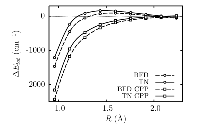
Figure 3: Difference between the VMC total energies, $\Delta E_{tot}$, and those provided by the CD model potential of coxon04 . Energy differences are shown for calculations performed with both TN (solid lines) and BFD (dashed lines) pseudopotentials, and both with (squares) and without (circles) the Li CPP potential. An offset is added such that $\Delta E_{tot}\rightarrow 0$ as $R\rightarrow\infty$.

Introducing the Li CPPshirley93 into the QMC calculations improves $E_{\rm ZP}$ and $Y_{10}$ significantly, but makes $D_{e}$ too large and $R_{e}$ too small. These “biases” in the calculated values are consistent with those found in previous MCSCF calculationsgadea06 using a different pseudopotential and CPP to those used here. It is therefore reasonable to attribute these biases in our results to a general deficiency of the pseudopotential+CPP model for the ionic cores.

Figure 3 shows these biases as the difference between the VMC total energies and the CD model potentialcoxon04 , with an energy offset added such that all curves approach zero for increasing $R$. All results show an underestimate of the total energy with decreasing $R$ of rapidly increasing magnitude, which we ascribe to the overlap of the pseudopotential core regions. For the calculations without the CPP an overestimate occurs near equilibrium, whereas when the CPP is included this becomes an underestimate of larger magnitude, and for all $R$. This general trend occurs for both pseudopotentials, such that at the equilibrium separation the BFD result is better than the TN result for no CPP, but the reverse is true when the CPP is introduced. The same trend also occurs for the equilibrium separation itself. Note that the improved CPP estimates for $Y_{10}$, $Y_{20}$, $Y_{11}$, and $E_{\rm ZP}$ correspond to superior 2^nd and higher order derivatives of the potential at $R_{e}$, so are more subtle in Fig. 3.

For all geometries considered, the change in total energy upon introduction of the CPP is very similar for both pseudopotentials. This is consistent with the suggestion of Shirley and Martinshirley93 that their CPPs are valid for use with different types of HF pseudopotential.

For many systems the computational cost of evaluating the integral required for the pseudopotential energy is very significant, and may even be dominant for DMC calculations in which the number of points in the integration grid, $N_{p}$, is large. The computational cost of the non-local integration depends on the size of the region inside the non-local radius, which is the distance beyond which the angular momentum components of the pseudopotential differ by less than some parameter $\epsilon$. The non-local radii of the tabulated TN pseudopotentials are consistently smaller than those of the BFD pseudopotentials. For $\epsilon=10^{-5}$ a.u. and Li, the non-local radii are $1.44$ Å (TN) and $1.66$ Å (BFD). For the DMC calculations considered here this resulted in a $14\%$ smaller computational cost when using the TN pseudopotentials. The advantage is smaller for VMC calculations. The cutoff radii of the TN pseudopotentials also depend less sensitively on the value of $\epsilon$. For example, with a tolerance of $10^{-4}$ a.u. the Li core radii are $1.40$ Å (TN) and $1.52$ Å (BFD) ($9\%$ greater), while for a tolerance of $10^{-8}$ a.u. the two radii are $1.54$ Å and $2.06$ Å, respectively (a $34\%$ increase). We emphasise that the tabulated TN pseudopotentials are intended for use in QMC calculations,trail05c while the Gaussian parameterisations are intended for use in quantum chemistry codes which require such a representation. For the latter, the non-local radius is larger, taking the value $1.69$ Å for $\epsilon=10^{-5}$ a.u.

VI Conclusions

Pseudopotentials are often used in ab initio calculations with very little account taken of the error introduced. In many cases, particularly for explicitly correlated calculations, the errors from the pseudopotential and the approximate method used to calculate the energies are not distinguished. We have chosen a system which is sufficiently small that we can solve it to very high accuracy using a variety of methods and for which a large amount of accurate experimental data is available. Anharmonic effects are very important for the LiH ground state and the prediction of its spectroscopic constants is a severe test of the theory. It is also worth mentioning that in the process of extracting the spectroscopic constants from the ab initio total energies an interatomic potential is generated with controlled accuracy.

We have compared pseudopotentials constructed from uncorrelated atomic calculations using different approaches, the “shape-consistent” or norm-conserving pseudopotentials of TN, and the “energy-consistent” pseudopotentials of BFD. The differences between the results obtained with the TN and BFD pseudopotentials are small compared with the differences from experiment. This conclusion holds whether or not the CPP is included. Introducing the CPP substantially improves the zero-point energy $E_{\rm ZP}$, but the harmonic equilibrium separation $R_{e}$, and well-depth $D_{e}$, are poorer.

The changes in the QMC estimates of $R_{e}$, $w_{e}$, and $D_{e}$ upon introducing the CPP are consistent with those found by previous authors using quantum chemistry methods, and their analysis of the source deficiencies of the CPP.othercpp However, the accurate description of the electron-electron cusp in the QMC calculations significantly improves the estimates of $w_{e}$ and $D_{e}$ over those found using quantum chemistry methods.

It appears that using a HF-based pseudopotential which does not contain correlation effects and adding the CPP which approximately describes core relaxation and core-valence correlation effects provides a reasonable model of LiH, but one which still suffers from significant errors. Whether these errors can be reduced by using a Li pseudopotential constructed using data from correlated calculations and/or by modifying the Li CPP is currently unknown.

- (1) W. M. C. Foulkes, L. Mitas, R. J. Needs, and G. Rajagopal, Rev. Mod. Phys. 73, 33 (2001).
- (2) A. Ma, N. D. Drummond, M. D. Towler, and R. J. Needs, Phys. Rev. E 71, 066704 (2005).
- (3) D. M. Ceperley, J. Stat. Phys. 43, 815 (1986).
- (4) J. R. Trail and R. J. Needs, J. Chem. Phys. 122, 174109 (2005).
- (5) J. R. Trail and R. J. Needs, J. Chem. Phys. 122, 014112 (2005).
- (6) M. Burkatzki, C. Filippi, and M. Dolg, J. Chem. Phys. 126, 234105 (2007).
- (7) J. L. Dunham, Phys. Rev. 41, 721 (1932).
- (8) J. A. Coxon and C. S. Dickinson, J. Chem. Phys. 121, 9378 (2004).
- (9) P. G. Hajigeorgiou and R. J. Le Roy, J. Chem. Phys. 112, 3949 (2000); Y. Huang and R. J. Le Roy, J. Chem. Phys. 119, 7398 (2003).
- (10) R. Maezono, A. Ma, M. D. Towler, and R. J. Needs, Phys. Rev. Lett. 98, 025701 (2007).
- (11) W. C. Stwalley and W. T. Zemke, J. Phys. Ref. Data 22, 87 (1993); A. G. Maki, W. B. Olsen, and G. Thompson, J. Mol. Spect. 144, 257 (1990).
- (12) M. W. Schmidt, K. K. Baldridge, J. A. Boatz, S. T. Elbert, M. S. Gordon, J. H. Jensen, S. Koseki, N. Matsunaga, K. A. Nguyen, S. J. Su, T. L. Windus, M. Dupuis, and J. A. Montgomery, J. Comput. Chem. 14, 1347 (1993).
- (13) R. J. Needs, M. D. Towler, N. D. Drummond, and P. López Ríos, casino version 2.1 User Manual, University of Cambridge, Cambridge (2007).
- (14) M. Casula, Phys. Rev. B 74, 161102 (2006).
- (15) N. D. Drummond, M. D. Towler, and R. J. Needs, Phys. Rev. B 70, 235119 (2004).
- (16) C. J. Umrigar, J. Toulouse, C. Filippi, S. Sorella, and R. G. Hennig, Phys. Rev. Lett. 98, 110201 (2007).
- (17) M. D. Brown, J. R. Trail, P. López Ríos, and R. J. Needs, J. Chem. Phys. 126, 224110 (2007).
- (18) J. R. Trail and R. J. Needs, http://www.tcm.phy.cam.ac.uk/mdt26/casino2_pseudopotentials.html.
- (19) E. L. Shirley and R. M. Martin, Phys. Rev. B 47, 15413 (1993).
- (20) C. J. Lorenzen and K. Niemax, J. Phys. B 15, 139 (1982).
- (21) L. Mitas, E. L. Shirley, and D. M. Ceperley, J. Chem. Phys. 95, 3467 (1991).
- (22) M. F. V. Lundsgaard and H. Rudolph, J. Chem. Phys. 111, 6724 (1999).
- (23) F. X. Gadea and T. Leininger, Theor. Chem. Acc. 116, 566 (2006).
- (24) C. Froese Fisher, G. Tachiev, G. Gaigalas, and M. Godefroid, Comput. Phys. Commun. 176, 559 (2007); http://atoms.vuse.vanderbilt.edu.
- (25) J. Kobus, L. Laaksonen, and D. Sundholm, Comput. Phys. Commun. 98, 346 (1996); http://scarecrow.1g.fi/num2d.html.
- (26) P. Fuentealba, O. Reyes, H. Stoll, and H. Preuss, J. Chem. Phys. 87, 5338 (1987); T. Leininger, A. Nicklass, W. Küchle, H. Stoll, M. Dolg, and A. Bergner, Chem. Phys. Lett. 255, 274 (1996); M. Dolg, Theor. Chim. Acta 93, 141 (1996).