Heavy-tailed random error in quantum Monte Carlo

Abstract

The combination of continuum Many-Body Quantum physics and Monte Carlo methods provide a powerful and well established approach to first principles calculations for large systems. Replacing the exact solution of the problem with a statistical estimate requires a measure of the random error in the estimate for it to be useful. Such a measure of confidence is usually provided by assuming the Central Limit Theorem to hold true. In what follows it is demonstrated that, for the most popular implementation of the Variational Monte Carlo method, the Central Limit Theorem has limited validity, or is invalid and must be replaced by a Generalised Central Limit Theorem. Estimates of the total energy and the variance of the local energy are examined in detail, and shown to exhibit uncontrolled statistical errors through an explicit derivation of the distribution of the random error. Several examples are given of estimated quantities for which the Central Limit Theorem is not valid. The approach used is generally applicable to characterising the random error of estimates, and to Quantum Monte Carlo methods beyond Variational Monte Carlo.

Quantum Monte Carlo (QMC) provides a means of integrating over the full $3N$-dimensional coordinate space of a many-body quantum system in a computationally tractable manner while introducing a random error in the result of the integrationfoulkes01 . The character of this random error is of primary importance to the applicability of QMC, and in what follows an understanding of the underlying statistics is sought for the special case of Variational Monte Carlo (VMC).

Within QMC, estimated expectation values have a random distribution of possible values, hence it is necessary to know the properties of this distribution in order to be satisfied that the statistical error is sufficiently well controlled. Many strategies (notably those involved in wavefunction optimisation and total energy estimation) sample quantities that exhibit singularities, and sample the singularities rarely. This is characteristic of a Monte Carlo (MC) strategy that is unstable and prone to abnormal statistical error due to outlierstraub98 .

In what follows the VMC method is analysed in order to obtain the statistical properties of the random error. Analytic results are obtained, and compared with the results of numerical calculations for an isolated all-electron carbon atom. The analysis naturally divides into four sections. Section I provides a summary of the implementation of MC used within VMC. The construction of estimated expectation value of an operator/trial wavefunction combination is described for the ‘standard sampling’ case (the most commonly used formfoulkes01 ) as a special case of a more general formulation. This short section provides no new results, but introduces the notation used throughout, and presents well established results from a perspective appropriate to the following sections.

Section II provides a transformation of the $3N$-dimensional statistical problem to an equivalent $1$-dimensional problem. The purpose of this section is to provide a simple mathematical picture of the statistical process that is entirely equivalent to the original $3N$-dimensional random sampling process. This is achieved by removing the statistical freedom in the system that is redundant for a given estimate. The principal result of this section is the derivation of a general statistical property that arises for almost all of the trial wavefunctions available for VMC calculations, and that may not easily be prevented. This statistical property dominates the behaviour of errors in VMC estimates, and the demonstration of its presence provides the starting point for the derivation of the statistics of estimators.

In section III the ‘standard sampling’ formulation of VMC is analysed. The goal is to find the distribution of the random error in statistical estimates of the total energy and the ‘variance’, for a finite but large number of samples. The principal conclusion of this section is that the Central Limit Theorem (CLT) is not necessarily valid and, when it is valid, finite sampling effects may be important even for a large sample size. This is demonstrated analytically, in the form of new expressions for the distribution of errors occurring for ‘standard sampling’ estimates of the total energy and variance. Numerical results for an isolated carbon atom provide an example of this effect for a calculation employing an accurate trial wavefunction.

In section IV estimates of several other quantities relevant to QMC are considered, and the invalidity of the CLT for these estimates is described (when derived using the same method as section III). This section directly relates to the infinite variance estimators that have previously been discussed in the literatureassaraf .

Finally, we note that this is the first of two closely related papers. It provides a general approach to rigorously deriving the statistics of the random error that is an inherent part of QMC methods, and uses this approach to obtain the statistical limitations of the simplest available sampling strategy. The following papertrail07b employs this new analysis of the statistics of QMC in order to design sampling strategies that are superior, in the sense that the Normal distribution of random errors can be reinstated for a given QMC estimate.

I ‘Standard sampling’ Variational Monte Carlo

The basic equation by which MC methods provide a statistical estimate for an integral may be written as

$$\frac{1}{r}\sum_{n=1}^{r}\frac{f(\text{R}_{n})}{P(\text{R}_{n})}=\int_{V}fd{\bf R}+\mathsf{W}_{r}$$ (1)

where $P$ is the probability density function (PDF) of the independent identically distributed (IID) $3N$-dimensional random vector $\text{R}_{n}$, and $\mathsf{W}_{r}$ is the random error in the estimate.

Introducing some notation used throughout the paper, the statistical estimate of a quantity $f$ constructed using $r$ samples is denoted $\mathsf{A}_{r}[f]$, hence Eq. (1) can be written as

$$\mathsf{A}_{r}\left[\int_{V}fd{\bf R}\right]=\mathbb{E}\left[\frac{f}{P};P\right]+\mathsf{W}_{r},$$ (2)

where the LHS is the statistical estimate of the integral (the sample mean in Eq. (1)), and the RHS can be interpreted as a sum of an expectation of a quantity $x=f/P$ sampled over the distribution with PDF $P$, and a random error. Whether the estimate is useful depends on the PDF of $\mathsf{W}_{r}$, specifically how this distribution evolves as $r$ increases.

An expectation value of the quantum mechanical operator $\hat{g}$ and (unnormalised) wavefunction, $\psi$, is defined by

$$G=\frac{\mathbb{E}\left[G_{L}\psi^{2}/P;P\right]}{\mathbb{E}\left[\psi^{2}/P;P\right]},$$ (3)

where $G_{L}=\psi^{-1}\hat{g}\psi$ is the ‘local value’ of the operator/trial wavefunction combination. By definition, VMC provides a MC estimate for this quantity, and since it is a quotient of two expectations it is more complex to estimate than a single integral.

‘Standard sampling’ is the most common and straightforward choice, for which samples are distributed as $P({\bf R})=\lambda\psi^{2}$, resulting in the simple form

$$\mathsf{A}_{r}\left[G\right] = \mathbb{E}\left[G_{L};\lambda\psi^{2}\right]+\mathsf{Y}_{r}$$ (4)

$$= \frac{1}{r}\sum_{n=1}^{r}G_{L}(\text{R}_{n}),\;\;\;\;P({\bf R})=\lambda\psi^{2},$$

where $\lambda$ need not be known since it is not required to generate samples distributed as $P({\bf R})$foulkes01 . This simple form arises from choosing $P$ such that the normalisation integral of Eq. (3) is sampled perfectly.

Within ‘standard sampling’ it is usually assumed that the CLT is valid, and that $r$ is large enough for the asymptotic limit to be reached to a required accuracy. If this is so, then $\mathsf{Y}_{r}$ is distributed normally with a mean of $0$, a variance given in terms of the sample variance

$$\mathrm{Var}\left[\mathsf{A}_{r}\left[G\right]\right]=\frac{1}{r}\;\mathsf{A}_{r}\left[\mathrm{Var}\left[G_{L}(\text{R}_{n})\right]\right],$$ (5)

and a confidence range for an estimated value can be obtained via the error function.

Two issues concerning the nature of the random error naturally suggest themselves. The use of the CLT to provide a confidence interval for the estimate implicitly assumes that the large $r$ limit has been reached. Whether this is the case for finite $r$ is a non-trivial questionstroock93 . The second issue is the validity of the CLT. Since this theorem is applicable to a limited class of distributions that may or may not include the distribution of samples within VMC (or other QMC methods) this is also a non-trivial question.

It is useful at this point to introduce some further definitions and notation. An estimate is a random variable, and random variables are denoted by a sans-serif font throughout. A particular sample value of an estimate is referred to as a sample estimate, and estimates are usually constructed from sums of random variables. The PDF of the estimate constructed from $r$ random variables is denoted $P_{r}(x)$, and defined by

$$\textrm{Prob}\left[a<\mathsf{A}_{r}\left[G\right]\leq b\right]=\int_{a}^{b}P_{r}(x)dx,$$ (6)

and an estimate is unbiased if it has a mean for a given $r$ that is equal to its true value. For the estimate to be useful the PDF of the error, $\mathsf{Y}_{r}$, must possess certain properties. It would be desirable for this PDF to approach a Dirac delta function for increasing $r$, and for some information to be available on the form of the PDF for finite $r$. In addition an estimate-able confidence range for finite $r$ is desirable, and zero mean value for $\mathsf{Y}_{r}$ for finite $r$.

II General asymptotic form for the distribution of local energies

For the standard implementation of VMC summarised in the previous section, the basic random variable is the $3N$-dimensional position vector of all the particles within the system, R. This is a ‘fundamental’ random variable in the sense that QMC is normally implemented as a random walk in the multidimensional space, $\mathbf{R}$. However, this random variable contains far more information than is required for many purposes. An analysis is given here for the expectation value of quantities that may be expressed in terms of the local energy, $E_{L}=\psi^{-1}\hat{H}\psi$. Note that this is a general procedure, and is applicable to estimates of any operator by defining a local field variable (scaler, vector or higher order) to remove the redundant statistical freedom present in the full $3N$-dimensional space, providing a more concise representation.

The expectation of a function of the local energy $E_{L}$ is defined as

$$\frac{\langle\psi|f(\hat{H})|\psi\rangle}{\langle\psi|\psi\rangle} = \mathbb{E}\left[f;\lambda\psi^{2}\right]$$ (7)

$$= \int P_{\psi^{2}}(\mathbf{R})f(E_{L})d\mathbf{R},$$ (8)

and the ‘standard sampling’ MC estimate of this is constructed by sampling the $3N$-dimensional coordinate vector over the ‘seed’ PDF $P_{\psi^{2}}(\mathbf{R})=\lambda\psi^{2}$.

Integrating over a hyper-surface of constant local energy removes redundant statistical degrees of freedom leaving the field variable, $E_{L}(\mathbf{R})$, as the random variable. The expectation is then given by

$$\mathbb{E}\left[f;P_{\psi^{2}}\right]=\int P_{\psi^{2}}(E)f(E)dE,$$ (9)

with the ‘seed’ PDF of the local energy given by

$$P_{\psi^{2}}(E)=\int_{\partial}\frac{P(\mathbf{R})}{\left|\nabla_{\mathbf{R}}E_{L}\right|}d^{3N-1}\mathbf{R},$$ (10)

where ${\partial}$ is a surface of constant $E_{L}$, and $\nabla_{\mathbf{R}}E_{L}$ is the gradient of the local energy in $3N$-dimensional space. The interpretation of this surface integral is straightforward, provided that disconnected surfaces and non-smoothness in the hyper-surface are dealt with as a sum of separate (and sometimes connected) surface integrals. Equation (10) simplifies the interpretation of general statistical properties considerably. Analytic properties of the seed distribution may be derived that are general to the $(\hat{H},\psi)$ combinations used for VMC.

In what follows we limit ourselves to the case of electrons in the potential of fixed atomic nuclei and Coulomb interactions, giving a local energy in $3N$-dimensional space of the form

$$E_{L}(\mathbf{R}) = -\frac{1}{2}\frac{\nabla^{2}_{\mathbf{R}}\psi}{\psi}+V_{ee}(\mathbf{R})+V_{ext}(\mathbf{R})$$ (11)

$$= T_{L}+V_{L},$$

where $V_{ee}(\mathbf{R})$ is the sum of two-body potentials (the electron-electron Coulomb interaction), and $V_{ext}(\mathbf{R})$ is the sum of one body potentials (the electron-nucleus Coulomb interaction). $T_{L}$ is the local kinetic energy, and all other terms are contained in $V_{L}$, the local potential energy. Singularities will occur for a general $\psi$, and the expression above naturally suggests classifying these into $4$ different types. Each has a characteristic influence on the asymptotic behaviour of $P_{\psi^{2}}(E)$, and an analysis of this relationship is given below.

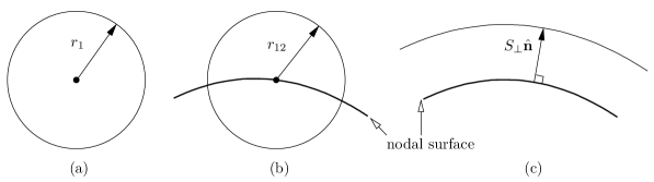
Figure 1: Constant energy surfaces in the large $E$ limit. Figure (a) shows the surface in terms of the electron-nucleus vector as coalescence is approached. The same geometry arises for electron-electron coalescence where the electrons possess different spin. Figure (b) shows the surface in terms of the electron-electron vector for electrons of like spin for the case where no singularity is present in the local kinetic energy. Figure (c) shows the constant energy surface for singularities at the nodal surface due to the local kinetic energy, $T_{L}$.

II.1 Type 1: electron-nucleus coalescence

Type 1 singularities are those resulting from any electron coordinate $\mathbf{r}_{i}$ approaching a singularity in the one body external potential $V_{ext}$, such as the $-Z/r$ behaviour of an atomic nucleus. This occurs on a $3N-3$ dimensional hyper-surface.

For a particular electron of coordinate $\mathbf{r}_{1}$ approaching a nucleus, the trial wavefunction can be expanded in spherical coordinates to give

$$\psi(\mathbf{r}_{1})=a_{0}(\mathbf{R}_{3N-3})+a_{1}(\Omega,\mathbf{R}_{3N-3})r_{1}+\ldots,$$ (12)

where $\mathbf{r}_{1}=(r_{1},\Omega)$ and $\mathbf{R}_{3N-3}$ is the ${3N-3}$ dimensional vector of the rest of the coordinate space. If $\psi$ does not possess singularities, it must be possible to expand $a_{n}(\Omega)$ as a closed sum of spherical harmonics $Y_{lm}(\Omega)$ with $l\leq n$. Similarly, for $\psi$ to be continuous up to order $n$, the coefficient $a_{n}(\Omega)$ must contain only odd/even $l$ spherical harmonics in its expansion for odd/even $n$.

For a trial wavefunction that is smooth at $r_{1}=0$ this results in a local energy of the form

$$E_{L}(\mathbf{R})-E_{0}=-\frac{Z}{r_{1}}+b_{0}(\mathbf{R}_{3N-3})+\ldots.$$ (13)

The absence of a $r_{1}^{-2}$ term is a direct consequence of $\psi$ being continuous at $r_{1}=0$, and the $r_{1}^{-1}$ term is entirely due to the presence of the nucleus potential and the derivative of $\psi$ being continuous at $r_{1}=0$. Figure 1(a) shows a 2D cut through the 3D space of $\mathbf{r}_{1}$, with $\mathbf{R}_{3N-3}$ held constant and the singularity due to the nucleus at the centre of the (asymptotically) spherical constant energy surface.

Rearranging and repeated re-substitution provides the integrand in Eq. (10), and integrating over the constant energy surface defined by the limit $E_{L}\rightarrow\pm\infty$ (a ‘hyper-tube’ which is spherical in the space of $\mathbf{r}_{1}$, but has no simple form in the $3N-3$ dimensions of $\mathbf{R}_{3N-3}$) gives the general form for the tail

$$P_{\psi^{2}}(E)=\left\{\begin{array}[]{ll}0&E\gg E_{0}\\ (E-E_{0})^{-4}\left(e_{0}+\frac{e_{1}}{(E-E_{0})}+\ldots\right)&E\ll E_{0}\end{array}\right.,$$ (14)

where $E\gg E_{0}$ ($E\ll E_{0}$) denotes an asymptotic expansion that converges for $E$ greater (less) than some finite value. The asymptotic behaviour is one sided since the singularity is negative, and the nodal surface does not need to be considered.

If the usual electron-nucleus Kato cusp conditionpack66 ; myers91 is forced on $\psi$ it introduces a discontinuity in the gradient at $r_{1}=0$ that exactly cancels the singular nucleus potential in the local energy via the local kinetic energy, hence this type of singularity can generally be removed. The cusp condition also introduces an $\Omega$ dependence in the $b_{0}$ term of the expansion, and hence a discontinuity in the local energy at the nucleus (although it is of zero size for some wavefunctions) . For $N$ electrons approaching the nucleus concurrently the same cusp conditions are sufficient to prevent a singularity, as discussed in the next section.

II.2 Type 2: electron-electron coalescence

Type 2 singularities may occur for $\mathbf{r}_{i}$ approaching $\mathbf{r}_{j}$ ($i\neq j$), and result from a singularity in the two-body electron-electron interaction, $V_{ee}$. The coalescence of electrons of like spin (indistinguishable) and unlike spin (distinguishable) must be considered separately. By transforming to centre of mass coordinates for the two electrons with positions vectors $\mathbf{r}_{1},\mathbf{r}_{2}$ defined as $\mathbf{r}_{12}=\mathbf{r}_{1}-\mathbf{r}_{2}$ and $\mathbf{s}_{12}=(\mathbf{r}_{1}+\mathbf{r}_{2})/2$ the same approach can be taken as for the electron-nucleus coalescence surfaces. To simplify the notation the vector $\mathbf{s}_{12}$ is included with the coordinates of the rest of the electrons in the vector $\mathbf{R}_{3N-3}$.

For distinguishable (unlike spin) electrons the situation in entirely analogous to the electron-nucleus case. The electron-nucleus vector and interaction is replaced by the electron-electron vector and interaction to give

$$P_{\psi^{2}}(E)=\left\{\begin{array}[]{ll}(E-E_{0})^{-4}\left(e_{0}+\frac{e_{1}}{(E-E_{0})}+\ldots\right)&E\gg E_{0}\\ 0&E\ll E_{0}\end{array}\right.,$$ (15)

where $E_{0}$ and the coefficients, $e_{n}$, are distinct from those in Eq. (14). (In order to keep the notation simple the same symbols are used for distinct coefficients in all of the series expansions contained within this section.) The asymptote is one sided due to the repulsive electron-electron interaction, and the nodal surface does not influence the result. Enforcing the Kato cusp condition for unlike spins removes these tails and introduces a discontinuity in the local energy in precisely the same manner as for the electron-nucleus coalescence.

For indistinguishable (like spin) electrons the situation is more complex. Figure 1(b) shows a 2D cut through the 3D space of $\mathbf{r}_{12}$, with $\mathbf{R}_{3N-3}$ held constant and a constant energy surface that is (asymptotically) spherical in the electron-electron coordinate. The singularity due to electron-electron coalescence is at the centre of the sphere. Unlike the distinguishable electron case the coalescence point must fall on the nodal surface, and the influence this has on $\psi$ must be taken into account.

Expanding a smooth antisymmetric trial wavefunction about the coalescence point (on the nodal surface) gives

$$\psi(\mathbf{r}_{12})=a_{1}(\Omega,\mathbf{R}_{3N-3})r_{12}+a_{3}(\Omega,\mathbf{R}_{3N-3})r_{12}^{3}+\ldots,$$ (16)

where interchange of electrons corresponds to inversion about $r_{12}=0$ so the coefficient $a_{n}$ contains only odd $l$ spherical harmonics and $l\leq n$. This provides a quadratic lowest order variation in the probability density perpendicular to the nodal surface, which results in a local energy of the form

$$E_{L}(\mathbf{R})-E_{0}=\frac{1}{r_{12}}+b_{1}(\Omega,\mathbf{R}_{3N-3})r_{12}+\ldots,$$ (17)

and an (asymptotically) spherical constant local energy surface centred at the coalescence point. Note that the absence of a $r_{12}^{-2}$ term is a direct consequence of the gradient of $\psi$ being continuous at $r_{12}=0$. The $r_{12}^{-1}$ term is entirely due to the Coulomb potential, together with $\psi$ being odd on interchange of electrons and possessing a continuous second derivative at $r_{12}=0$. Performing the ‘hyper-tube’ integration then gives

$$P_{\psi^{2}}(E)=\left\{\begin{array}[]{ll}(E-E_{0})^{-6}\left(e_{0}+\frac{e_{1}}{(E-E_{0})}+\ldots\right)&E\gg E_{0}\\ 0&E\ll E_{0}\end{array}\right.,$$ (18)

where, since the singularity is positive, the asymptotic behaviour is one sided.

Enforcing the Kato cusp conditionpack66 ; myers91 for like spins introduces a second order radial term, with coefficient $a_{2}=a_{1}/4$. This provides a discontinuity in the $2^{nd}$ order derivatives of $\psi$ at $r_{12}=0$ that cancels the singular electron-electron interaction, and so removes the tails due to the like spin electron-electron coalescence. A further consequence is a continuous local energy as the coalescence plane is crossed, with a discontinuity in the gradient of the local energy.

So far only electron-nucleus and electron-electron coalescence has been considered. For the general case of many electron coalescence (some distinguishable, some not) at a nucleus site, or at any point in space, and a smooth trial function $\psi$, the local energy may be written in the form

$$E_{L}(\mathbf{R})-E_{0}=\sum_{i}\frac{Z}{r_{i}}+\sum_{i<j}\frac{1}{r_{ij}}+\ldots$$ (19)

provided that the local kinetic energy is smooth. As discussed by Packpack66 , provided the trial wavefunction satisfies the cusp conditions for each electron-electron and electron-nucleus coalescence, then the Coulomb singularities will exactly cancel with singularities in the local kinetic energy. These conditions are easily satisfied for trial wavefunctions that are a function of electron-nucleus, electron-electron and electron-electron-nucleus coordinates, but for higher order correlations internal coordinates must be considered explicitly.

Although the Kato cusp conditions remove the Coulomb singularities from the local energy, they do not prevent the occurrence of discontinuities on the same hyper-surface of electron-nucleus and electron-electron coalescence. Further cusp conditions that remove these discontinuities may be obtained directly from the local energy expansions given above.

II.3 Type 3: nodal surface

The third type of singularity (and associated tails in the seed distribution) occurs for almost all of the trial wavefunctions used in QMC calculations, with the exception of some few electron systems.

Type 3 singularities are due to the kinetic energy only, and occur at the nodal surface due to the presence of $\psi$ in the denominator of the expression for the local kinetic energy. There is no equivalent to the previous cusp conditions that can easily be enforced on $\psi$ to prevent these type 3 singularities occurring, and they are of a fundamentally different nature.

Proceeding in a similar manner to the previous two cases, the trial wavefunction is expanded about the singular surface, in this case the $3N-1$ dimensional nodal surface. This expansion is then used to provide a constant local energy hyper-surface, over which an integral is performed to obtain the PDF in energy space.

Figure 1(c) shows a 2D cut through the $3N$ dimensional space that includes the nodal surface, and a constant local energy surface at a perpendicular distance $S_{\perp}$ from the nodal surface. Expressing the vector of a point on the constant energy surface as

$$\mathbf{R}=\mathbf{X}+S_{\perp}\hat{\mathbf{n}},$$ (20)

where $\mathbf{X}$ is a point on the nodal surface, and $\hat{\mathbf{n}}(\mathbf{X})=\widehat{\nabla_{\mathbf{R}}E_{L}}\left|{}_{\mathbf{X}}\right.$ is the normalised gradient at $\mathbf{X}$, gives

$$\psi(\mathbf{R})=a_{1}(\mathbf{X})S_{\perp}+a_{2}(\mathbf{X})S_{\perp}^{2}+\ldots$$ (21)

and

$$E_{L}(\mathbf{R})-E_{0}=b_{-1}(\mathbf{X})S_{\perp}^{-1}+b_{0}(\mathbf{X})+b_{1}(\mathbf{X})S_{\perp}+\ldots.$$ (22)

Employing these in Eq. (10) and integrating over the constant energy surface defined by the limit $E_{L}\rightarrow\pm\infty$ (the nodal surface) gives the general form

$$P_{\psi^{2}}(E)=\left.\begin{array}[]{ll}(E-E_{0})^{-4}\left(e_{0}+\frac{e_{1}}{(E-E_{0})}+\ldots\right)&\ \ \ \ |E|\gg E_{0}\end{array}\right..$$ (23)

Equation (23) tells us that for a general trial wavefunction and Hamiltonian the resulting ‘seed’ probability distribution in energy space has this asymptotic form for type 3 singularities. This result is central to the rest of this paper.

A special case of this type of singularity arises for a trial wavefunction where a nodal pocket is at the critical point of appearing/disappearing, which may occur in the process of varying a parameterised trial wavefunction in the search for an optimum form. This occurs where a solution of the equation $\psi=0$ disappears, or for a local maximum/minimum of $\psi$ crossing the nodal surface. At this critical point $\psi=0$ defines a single point in $3N$ dimensional space, and the wavefunction may be expanded about this point using hyper-spherical coordinates $\mathbf{R}=(R,\mathbf{\Omega})$ (with $R$ the hyper-radius and $\mathbf{\Omega}$ the $3N-1$ hyper-angles) as

$$\psi(\mathbf{R})=a_{2}(\mathbf{\Omega})R^{2}+a_{3}(\mathbf{\Omega})R^{3}+\ldots.$$ (24)

The associated local energy then takes the form

$$E_{L}(R,\mathbf{\Omega})-E_{0}=b_{-2}(\mathbf{\Omega})R^{-2}+b_{-1}(\mathbf{\Omega})R^{-1}+b_{0}(\mathbf{\Omega})+\ldots$$ (25)

with the singular behaviour arising via the local kinetic energy. Following the same approach as for type 1 and type 2 singularities, but integrating over the surface of the hyper-sphere gives

$$P_{\psi^{2}}(E)=\frac{1}{\left|E-E_{0}\right|^{(3N+6)/2}}\left(e_{0}+\frac{e_{1}}{(E-E_{0})}+\ldots\right),$$ (26)

an asymptotic tail in the PDF that is one sided since the constant energy surface exists only in the nodal pocket that is not being created/annihilated. This gives a faster decay than $E^{-4}$ for $N\geq 1$, and nodal pockets can only occur in the ground state for $N\geq 2$. Consequently, this effect is secondary to the $E^{-4}$ behaviour arising from nodal surfaces that are not being created/annihilated, and will only dominate if annihilation of the nodal pocket results in no nodal surfaces anywhere in space. This can only occur if all fermions in the system are distinguishable.

II.4 Type 4: arbitrary bound trial wavefunctions

Singularities in the local energy may also occur if the local energy approaches infinity as any or all electrons approach an infinite distance from the nuclei or each other. This type of singularity is referred to as type 4, and its source may be the local kinetic energy, the local potential energy, or both, and can only occur for systems that do not extend over all space.

For these finite systems a reasonable assumption about the general form of a trial wavefunction used in QMC is that it is a bound state of some ‘model’ Hamiltonian (this encompasses the exact, HF, MCSCF, Kohn-Sham, Gaussian basis wavefunctions, and many others, with or without a Jastrow factor or backflow transformation). Hence, for the types of wavefunction that are used in QMC calculations, the asymptotic behaviour can be written as

$$\psi(\mathbf{R})\propto\left|\mathbf{R}\right|^{\alpha}e^{-\beta\left|\mathbf{R}\right|^{\gamma}},$$ (27)

where the parameters $\alpha$, $\beta$, and $\gamma$ depend on the type of trial wavefunction.

Following the same approach as for type 1 and 2 singularities, the influence on the asymptotic tails of the seed distribution can be determined by integrating over the constant local energy surface. This tells us that for $\gamma>1$ (e.g., a Gaussian basis set) $P_{\psi^{2}}$ decays as an exponential function of a power of $E$, whereas for $0<\gamma\leq 1$ ($\gamma=1$ is the correct asymptotic form) $P_{\psi^{2}}$ is zero outside of an energy interval (assuming that none of the other 3 types of singularity are present). The second case is preferable, but the former is not significant as it can only result in the presence of exponentially decaying tails in $P_{\psi^{2}}$. In what follows type 4 singularities are irrelevant.

Type 3 tails occur for almost all many body trial wavefunctions, with some exceptions. First, it is possible for there to be no nodal surface. This does not occur for systems containing two or more indistinguishable fermions, and does occur if the trial wavefunction is a bosonic ground state. Second, the nodal surfaces may be exactly known from symmetry considerations, as discussed by Bajdich et al.bajdich05 . A third exception arises from considering an effective Hamiltonian for which the trial wavefunction is an exact solution. This has a potential defined by

$$V_{eff}=E_{eff}+\frac{1}{2}\frac{\nabla^{2}_{\mathbf{R}}\psi}{\psi},$$ (28)

where $E_{eff}$ is arbitrary, but is usually chosen to be zero for a completely ionized system. If $V_{eff}$ can be shown to possess no singularities at the nodal surface, then $\nabla^{2}_{\mathbf{R}}\psi=0$ at the nodal surface and type 3 tails do not occur. An example is the Slater determinant, as this is the exact solution for fermions in a one-body potential (with no two-body or higher interactions present in $V_{eff}$). (Note that the available modifications of such ‘exact model’ solutions, such as Jastrow factors, result in a many-body $V_{eff}$ that is singular at the nodal surface.)

Removing type 3 singularities is a non-trivial problem since it is necessary to ensure that $T_{L}$ remains finite over the nodal surface apart from on the coalescence planes, where it must possess a singularity that exactly cancels the electron-electron Coulomb interaction. Type 3 tails are taken to be unavoidable in practice.

In order to clarify when these singularities/tails occur it is worth considering some examples. For an exact wavefunction none of the singularity types occur. For a Hartree-Fock or Kohn-Sham Slater determinant with no basis set error only type 2 singularities occur, since the electron-nucleus cusp conditions are satisfied, the asymptotic wavefunction behaviour has the correct exponential form, and the local kinetic energy is finite at the nodal surface. For a Hartree-Fock or Kohn-Sham Slater determinant with a Gaussian basis set, singularities of all four types occur, but type 1 and 2 singularities can be expected to dominate.

Figure 2: Variation of the local energy in the presence of singularities of all four types, with an electronic coordinate, ${\bf r}_{1}$, passing through singular hyper-surfaces. $I$, $II$, $III$, and $IV$ denote singularities due to e-n interaction, e-e interaction, the nodal surface, and incorrect asymptotic behaviour (shown here for the Gaussian case), respectively. Units are arbitrary.

Figure 2 shows a schematic of the form taken by the singularities in the local energy as an electron passes through the nucleus, through a coalescence plane, through a nodal surface, and continues away from the nucleus, for the case where all types of singularity are present. From this point on, only the influence of type 3 singularities and the associated symmetric tails in the seed distribution are considered, since type 1 and type 2 behaviour is easily and routinely removed, and type 4 behaviour does not affect the analysis that follows. It is the presence of these ‘leptokurtotic’ power law tails (also known as ‘heavy tails’, or ‘fat tails’) in the PDF of the sampled energies that provides the starting point for an analysis of random errors in the estimates of expectation values within VMC.

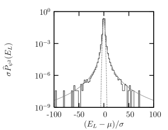
Figure 3: The seed probability density function estimated by a histogram of $r=10^{7}$ sampled local energies (black). These are results for an accurate all-electron carbon trial wavefunction, as described in the text. Shown in grey is the model distribution of Eq. (23) that reproduces the mean and variance of the samples, and the dotted line is the Normal distribution that reproduces the same mean and variance.

Before commencing, it is useful to explicitly show the presence and magnitude of the type 3 singularities for a real system, the isolated all-electron carbon atom. A numerical Multi-Configuration-Hartree-Fock calculation was performed to generate a multideterminant wavefunction consisting of $48$ Slater determinants (corresponding to 7 configuration state functions (CSF)) using the ATSP2K code of Fischer et al.fischer07 Further correlation was introduced via a $83$ parameter Jastrow factordrummond04 , and a $130$ parameter backflow transformationrios06 . This $219$ parameter trial wavefunction was optimised using a standard variance minimisation methodcasino06 , resulting in $E_{VMC}=-37.83449(7)$ a.u., compared with the ‘exact’chakravorty93 result of $-37.8450$ a.u. Of those trial wavefunctions that can practically be constructed and used in QMC this may be considered to be accurate, and reproduces $93.3\%$ of the correlation energy at the VMC level.

As discussed above, only type 3 singularities contribute to the asymptotic behaviour of the seed distribution. Figure 3 shows an estimate of the seed PDF, $P_{\psi^{2}}(E)$, constructed by taking $10^{7}$ standard samples of the local energy, binning these into intervals, and normalisingizenman91 . Also shown is a simple analytic form

$$p(E)=\frac{\sqrt{2}}{\pi}\frac{\widehat{\sigma}^{3}}{\widehat{\sigma}^{4}+\left(E-\widehat{E}_{tot}\right)^{4}},$$ (29)

and a Normal distribution, both with a mean and variance of $\widehat{E}_{tot}$ and $\widehat{\sigma}^{2}$ whose values are obtained from the data using the usual unbiased sample estimates.

It is apparent that the seed distribution, $P_{\psi^{2}}(E)$, is not well described by a Normal distribution. Considering that no fitting procedure is employed (beyond matching the first two moments of the model and sample distributions) it is somewhat surprising that the simple model distribution is so close to the actual distribution. This is most clearly demonstrated by comparing the number of sample points predicted in a ‘tail region’ defined by $(E-\widehat{E}_{tot})>10\widehat{\sigma}=2.25$ a.u. The numerical data has $2990$ sample points in this region, $p(E)$ predicts $3481$ points, and the Normal distribution predicts $1.7\times 10^{-14}$ points.

An alternative measure is to assume the asymptote

$$p_{asym}(E)=\frac{\sqrt{2}}{\pi}\frac{\lambda_{3}}{\widehat{\sigma}}\left(\frac{\widehat{\sigma}}{E-\widehat{E}_{tot}}\right)^{4}$$ (30)

to be dominant in the ‘tail region’, and to equate the sampled and predicted number of outliers. This estimates the magnitude of the leptokurtotic tails to be $\lambda_{3}=0.86$ (in comparison with $\lambda_{3}=1$ for the model distribution of Eq. 29).

Figure 3 suggests that the local energy is not well sampled close to the nodal surface, where the deviation from the mean is greatest. Further suspicion that a more detailed analysis is required arises when it is noted that third or higher moments do not exist for this seed distribution, even though a finite number of samples will provide an estimate of these higher moments that converges to infinity as the sample size is increased.

III Random error in VMC estimates

In the previous section no mention of MC methods has been made. In this section the consequence of choosing the ‘standard sampling’ strategy in QMC is investigated.

It has been noted by previous authors that for many calculations the distribution of the local energy is clearly not Gaussian, for both VMC and DMC calculationsbressanini02 ; kent99 ; bianchi88 ; pandharipande86 . Section II shows that this is generally the case. In previous work it also appears to be implicitly assumed that the form of the seed distribution is irrelevant to the application of the CLT to infer information on the random error of estimated quantitiesfoulkes01 . In what follows, the influence of the leptokurtotic tails on the validity of the CLT is examined in detail, and the distribution of random error in VMC estimates is derived.

Numerical evidence for a valid CLT is at best limited, and only weakly suggestive. For most applications of QMC only single estimates are constructed, with an estimated random error calculated using the CLT. Generally no ensemble of estimates is calculated to justify that this error is Normal. The best we can do is observe that for many published results the estimated total energies and errors are consistent with exact energies where these are known in that they are higher (to within the statistical accuracy suggested by the CLT). This still leaves significant room for non-Gaussian error, especially for larger systems and estimates of quantities other than the total energy.

Results for wavefunction optimisation within VMC are more strongly suggestive. The most stable implementation possible for a stochastic minimisation method would provide a Normal random error in the optimised functional. Instability is commonly observed for many of the available implementations, particularly for a large number of particles or where the nodal surface of the trial wavefunction is variedkent99 ; bressanini02 . This is consistent with the notion that the CLT may not be valid for these implementations.

Possible distributions of error in estimates can be summarised as follows. The catastrophic case would be for the Law of Large numbers to be invalid, providing estimates that do not statistically converge to an expectation as $r$ approaches infinity. Another possibility is that the Central Limit Theorem may not be valid, providing estimates that statistically converge, but with a random error that is not Normally distributed. A further possibility is that the CLT may be valid, but that the deviation from the Normal distribution for finite $r$ is unknown, so may be significant for accessible sample sizes. A final, ideal case would be for the CLT to be valid, and for the deviation from the Normal distribution for finite $r$ to be known, and to be unimportant for accessible sample sizes.

The first and last of these are found not to occur, while the other cases do (depending on what is being estimated), as a direct consequence of the presence of the leptokurtotic tails.

III.1 Total energy

As discussed in section I, the unbiased estimate of the total energy constructed from local energy values at $r$ points sampled from the $P_{\psi^{2}}$ distribution is given by

$$\mathsf{A}_{r}\left[E_{tot}\right]=\frac{1}{r}\sum_{n=1}^{r}\mathsf{E}_{n},$$ (31)

with $\{\mathsf{E}_{n}\}$ the IID random variables $E_{L}(\text{R})$. This (rescaled) sum of IID random variables can be analysed using the known properties of the PDFs of each $\mathsf{E}_{n}$ to obtain the PDF of the estimate itself.

It is useful to introduce some supplementary random variables in order to keep the notation simple. Defining the mean and variance of $P_{\psi^{2}}$ as $\mathbb{E}\left[E_{L}\right]$ and $\sigma^{2}$ provides the transformation

$$\mathsf{X}_{n}=\frac{1}{\sigma}\left(\mathsf{E}_{n}-\mathbb{E}\left[E_{L}\right]\right),$$ (32)

as long as the first two moments exist. This $\mathsf{X}_{n}$ has a PDF, $p(x)$, of mean and variance of $0$ and $1$, and a symmetric asymptotic behaviour $\propto 1/x^{4}$. Two further random variables are $\mathsf{S}_{r}$, defined as the sum of $r$ independent samples taken from $p(x)$, and the normalised version of this sum,

$$\mathsf{Y}_{r}=\frac{(\mathsf{X}_{1}+\ldots+\mathsf{X}_{r})}{\sqrt{r}}=\frac{\mathsf{S}_{r}}{\sqrt{r}}.$$ (33)

The transformation from $\mathsf{Y}_{r}$ to $\mathsf{A}_{r}\left[E_{tot}\right]$ is

$$\mathsf{A}_{r}\left[E_{tot}\right]=\frac{\sigma}{\sqrt{r}}\mathsf{Y}_{r}+\mathbb{E}\left[E_{L}\right],$$ (34)

so that $\mathsf{Y}_{r}$ is the random error in the estimate of the total energy in units of $\sigma/\sqrt{r}$.

The validity of the CLT for these sums of random variables is tested below, for the three most common forms of the CLT available. These are considered in order of increasing generality (in that they are valid for progressively larger classes of PDFs) and decreasing knowledge of finite sampling effects (in that limits on the deviation from normality for finite $r$ are progressively less well defined).

The least general CLT is provided by the existence or not of an Edgeworth series expansionstroock93 . Provided that all the moments of $p(x)$ exist, and that they satisfy Carleman’s conditionstroock93 , then the distribution of $\mathsf{Y}_{r}$ for $r$ samples, $P_{r}\left(y\right)$, can be uniquely defined by the infinite series

$$P_{r}\left(y\right)=\frac{1}{\sqrt{2\pi}}e^{-y^{2}/2}\left(1+\frac{f_{3}(y)}{\sqrt{r}}+\frac{f_{6}(y)}{r}+\ldots\right),$$ (35)

where each $f_{m}(y)$ is a finite polynomial in $y$ of order $m$, and with coefficients that may be expressed in terms of the first $m$ moments of the seed distribution. If this expansion is valid, $P_{r}\left(y\right)$ converges to the Normal distribution for increasing $r$, and the expansion also provides a definite bound on the deviation of the distribution from Normal for finite $r$ - the deviation can be estimated if necessary, and scales as the Gaussian function. For the seed distribution of local energies, $P_{\psi^{2}}$, the asymptotic behaviour ensures that all moments higher than $2^{nd}$ do not exist, hence this form of the CLT is invalid.

A more general result is the Berry-Esseen theoremstroock93 , which states that the inequality

$$\left|\int_{-\infty}^{x}P_{r}\left(y\right)-\frac{1}{\sqrt{2\pi}}e^{-y^{2}/2}dy\right|\leq\frac{C}{\sigma^{3}\sqrt{r}}\int_{-\infty}^{\infty}|y|^{3}p(y)dy,$$ (36)

is valid provided the $3^{rd}$ absolute moment on the RHS is finite ($C=0.7655$ is the best value of $C$ availablesenatov98 ). This proves that $P_{r}\left(y\right)$ converges to the Normal distribution for increasing $r$, and also provides a bound on the deviation of the distribution from Normal for finite $r$. The asymptotic behaviour of the seed distribution ensures the nonexistence of the $3^{rd}$ absolute moment, hence this form of the CLT is invalid for $P_{\psi^{2}}$.

The final candidate is Lindeberg’s theoremstroock93 . This is the most general form of the CLT, and provides the weakest bound on the deviation from Normality for finite $r$. Provided that

$$\textrm{Max}\left[\frac{|\phi(y)|}{1+y^{2}}\right]<\infty,$$ (37)

it follows that

$$\lim_{r\rightarrow\infty}\int_{-\infty}^{x}P_{r}\left(y\right)\phi(y)dy=\frac{1}{\sqrt{2\pi}}\int_{-\infty}^{x}\phi(y)e^{-y^{2}/2}dy,$$ (38)

or that in the limit of $r$ approaching infinity the probability of the sum of random variables falling in a given interval (given by $\phi(y)=1$) is equal to that of the Normal distribution provided by the CLT, provided that the $2^{nd}$ moment of $p(x)$ exists. This provides confidence limits from the sample mean and variance via the CLT for large $r$, but two points must be borne in mind. First, for $\phi(y)$ increasing faster than second order (such as the definition of moments higher than $2^{nd}$ order) the expectation is not defined, even in the limit of $r$ approaching infinity. Second, for finite $r$ there is no limit to the magnitude of any deviation from Normal, or to how fast these deviations decay with increasing $r$.

These theorems inform us that the random error in the unbiased estimate of the total energy obeys the CLT, but no information is available about the deviation of the distribution of errors from Normal for finite $r$. This is unsatisfactory, since only a finite number of samples will ever be available.

Using the asymptotic behaviour derived in section II does allow us to extract information about the deviation from Normal that appears in $P_{r}\left(y\right)$. In what follows this is achieved by using the same strategy as the most frequently presented derivation of the CLTgnedenko68 , but explicitly taking into account the leptokurtotic tails.

Denoting the PDF of the sum $\mathsf{S}_{r}$ as $P_{r}(s_{r})$ (distinct from $P_{r}\left(y\right)$ but related via a change of variables) and viewing this sum as a random walk in one dimension leads immediately to the iterative convolutions

$$P_{r}(s_{r})=p(x_{r})\star P_{r-1}(s_{r-1}),$$ (39)

starting from $P_{1}(s_{1})=p(x_{1})$. In Fourier space this is simply a product, and defining the Fourier transform as

$$p(k)=\int_{-\infty}^{\infty}p(x)e^{-ikx}dx$$ (40)

immediately gives

$$P_{r}(k)=e^{r\ln p(k)},$$ (41)

with $P_{r}(k)$ and $p(k)$ the characteristic functions of $P_{r}(s_{r})$ and $p(x)$ respectively. Equation (41) reduces the problem to that of finding the inverse Fourier transform of the $r^{th}$ power of the Fourier transform of the seed distribution (with an appropriate transformation of the random variables).

For a PDF to possess a smooth characteristic function (in the sense that all derivatives exist at all points), the PDF must decay at least exponentially fast as $|x|\rightarrow\infty$morse53 . If this were the case, then a Taylor expansion would exist for $\ln p(k)$ that is valid for all real $k$. For the distribution of local energies, the PDF falls to zero algebraically slowly which implies the presence of poles in the complex plane for finite $|x|$, discontinuities in the Fourier transform at the origin, and no Taylor series expansion about $k=0$ for $\ln p(k)$.

The Fourier transform may be performed by contour integration in the complex plane, closing the contour in the upper half plane for $\Re[k]<0$, and the lower half plane for $\Re[k]>0$. This, in addition to the constraints on the residues and the position of the poles that prevent any slower asymptotic behaviour, provides a general series expansion

$$\ln p(k)=-\frac{1}{2}k^{2}+\frac{\lambda_{3}}{3\sqrt{2}}\left|k\right|^{3}+\eta_{3}\left(ik\right)^{3}+\mathcal{O}\left(k^{4}\right).$$ (42)

All of the coefficients in this expansion are completely unrelated to moments of the seed distribution, and for the model distribution shown in Fig. (3), $\lambda_{3}=1$ and $\eta_{3}=0$. Higher order discontinuities may also be present in this expansion, as generally a $|x|^{-q}$ term in the asymptotic behaviour of a function is accompanied by a $|k|^{q-1}$ term in its Fourier transform due to the properties of bilateral Laplace transformsmorse53 .

This series expansion provides the required expression for $P_{r}(k)$,

$$P_{r}(k)=\exp\left[-r\frac{1}{2}k^{2}+r\frac{\lambda_{3}}{3\sqrt{2}}\left|k\right|^{3}+r\eta_{3}\left(ik\right)^{3}+\mathcal{O}\left(k^{4}\right)\right].$$ (43)

Changing variables to $w=\sqrt{r}k$ and $y=s_{r}/\sqrt{r}$ and performing the inverse Fourier transform gives

$$P_{r}(y) = \frac{1}{2\pi}\int_{-\infty}^{\infty}e^{iwy-w^{2}/2}\exp\left[\frac{\lambda_{3}}{3\sqrt{2}}\frac{1}{\sqrt{r}}\left|w\right|^{3}\right.$$ (44)

$$\left.+\eta_{3}\frac{1}{\sqrt{r}}\left(iw\right)^{3}+\mathcal{O}\left(\frac{w^{4}}{r}\right)\right]dw,$$

where the lowest order terms that are independent of $r$ have been factored out. Expanding the exponential whose argument is a function of $r^{-1}$ as an asymptotic series in $r$ gives

$$P_{r}(y)=\phi_{0}(y)+\frac{\lambda_{3}}{3\sqrt{2}}\frac{1}{\sqrt{r}}\chi_{3}(y)+\eta_{3}\frac{1}{\sqrt{r}}\phi_{3}(y)+\cdots$$ (45)

where $\phi_{0}(y)$ is the standard Normal distribution,

$$\chi_{q}(y)=\frac{1}{2\pi}\int_{-\infty}^{\infty}\left|w\right|^{q}e^{iwy-w^{2}/2}dw$$ (46)

and

$$\phi_{q}(y)=\frac{1}{2\pi}\int_{-\infty}^{\infty}(iw)^{q}e^{iwy-w^{2}/2}dw.$$ (47)

Higher order terms can be written in the same form, and will have a prefactor proportional to $r^{1-q/2}$. Note that $\chi_{q}$ and $\phi_{q}$ are distinct only for odd $q$.

Since $\phi_{0}(y)$ is a Gaussian function, the CLT is valid, and the PDF may be expressed as

$$P_{r}(y) = \frac{1}{\sqrt{2\pi}}\left[1+\frac{\eta_{3}}{\sqrt{r}}\frac{d^{3}}{dy^{3}}+\mathcal{O}\left(\frac{1}{r}\right)\right]e^{-y^{2}/2}$$ (48)

$$+\left[\frac{\lambda_{3}}{3\pi}\frac{1}{\sqrt{r}}\frac{d^{3}}{dy^{3}}+\mathcal{O}\left(\frac{1}{r}\right)\right]D\left(\frac{y}{\sqrt{2}}\right),$$

where $D(x)$ is the Dawson integralmorse53 defined by

$$D\left(x\right)=e^{-x^{2}}\int_{0}^{x}e^{t^{2}}dx,$$ (49)

and possessing finite derivatives of all orders, and a known asymptotic expansion. Further terms can be included explicitly if required, as higher order derivatives of the Gaussian function and Dawson integral.

In a region close to the mean, Eq. (48) may be expanded in the form

$$\lim_{|y|\rightarrow 0}P_{r}(y)=\left[\frac{1}{\sqrt{2\pi}}+\frac{1}{\sqrt{r}}h_{1}\left(y\right)+\mathcal{O}\left(\frac{1}{r}\right)\right]e^{-y^{2}/2},$$ (50)

where $h_{1}$ is an infinite series that converges over a finite region surrounding the mean. This expansion differs from the Edgeworth series in that it does not converge for all $y$.

Far from the mean, where the previous series expansion does not converge, the asymptotic behaviour takes the form

$$\lim_{|y|\rightarrow\infty}P_{r}(y)=\left[\frac{\sqrt{2}}{\pi}\frac{\lambda_{3}}{\sqrt{r}}\frac{1}{y^{4}}+\frac{1}{\sqrt{r}}\frac{1}{y^{6}}h_{2}\left(\frac{1}{y^{2}}\right)+\mathcal{O}\left(\frac{1}{r}\right)\right],$$ (51)

with $h_{2}(x)$ an infinite series that converges over a finite region surrounding $x=0$. This form arises because the second sum in Eq. (48) dominates for large $y$ (it is obtained from the asymptotic form of the derivative of the Dawson integral), and is fundamentally different in character to the Gaussian decay that would occur were an Edgeworth series to exists.

The model seed distribution introduced in the discussion of the all-electron carbon VMC results of the previous section corresponds to the special case $\lambda_{3}=1$ and $h_{1}=h_{2}=0$, and is the simplest form that results in this ‘persistent leptokurtotic’ behaviour for the distribution of total energy estimates.

These results allow some general observations about the distribution of errors in total energy estimates. As expected, the Normal distribution emerges in the large $r$ limit. However, for finite $r$ the character of the deviation far from the mean is dominated by $E^{-4}$ tails. The magnitude of these tails, $\lambda_{3}$ is not expressible in terms of moments of the samples, but is required in order to decide whether these leptokurtotic tails are statistically significant.

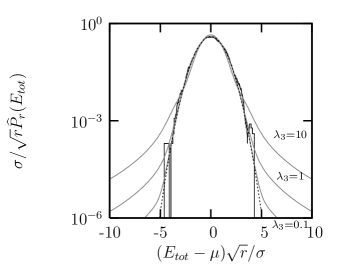
Figure 4: Probability density function for the random error in the estimated total energy. Results shown are for a kernel estimate of the PDF resulting from $10^{4}$ estimates with $r=10^{3}$ for each estimate (black). Grey lines show the predicted distribution, including leptokurtotic tails, for different $\lambda_{3}$ values. For comparison, the Normal distribution that emerges in the large $r$ limit is also shown (dotted line).

Figure 4 shows the distribution of errors, ($P_{r}$ of Eq. (48) truncated to order $1/r^{1/2}$), for a range of $\lambda_{3}$ values and $\eta_{3}=0$ (a non-zero value would introduce some asymmetry close to the mean). A non-zero $\lambda_{3}$ causes a redistribution of probability in an inner region where the Gaussian contribution to the density is dominant, with a net shift of probability to an outer region where the Gaussian contribution is vanishingly small and the leptokurtotic tails dominate.

A useful indicator of the impact of the leptokurtotic tails on confidence limits can be extracted as follows. The deviation from the mean (in units of standard error) at which the leptokurtotic tail starts to dominate can be defined as the intersection of the dominant parts of the asymptotic and small $y$ expansion of the distribution. This provides the equation

$$y_{c}^{2}=\ln\left(\frac{\pi r}{4\lambda_{3}^{2}}\right)+4\ln y_{c}^{2},$$ (52)

which may be solved numerically, and whose solution depends weakly on $r/\lambda_{3}^{2}$ due to the logarithmic term. Specifying extreme values of $r<10^{6}$ and $\lambda_{3}>1$ results in $y_{c}<5.2$. The value $y_{c}=4$ is chosen to be representative as it defines the $99.994\%$ confidence interval for a Gaussian distribution. Using this crossover point naturally defines a ‘Gaussian interval’ by $|y|<4$, and a ‘leptokurtotic interval’ by $|y|\geq 4$. Table 1 shows the probabilities resulting from a seed distribution with varying $r/\lambda_{3}^{2}$ values, where a typical value for the carbon atom calculations of section II is $(r,\lambda_{3})=(10^{4},1.0)$ or $r/\lambda_{3}^{2}=10^{4}$.

		$\mathrm{Prob}\ (\%)$
$r/\lambda_{3}^{2}$	$\lambda_{3}$	$|\mathsf{y}|\leq 4$	$|\mathsf{y}|\geq 4$
$\infty$	0.0	99.994	0.006
$10^{6}$	0.1	99.993	0.007
$10^{4}$	1.0	99.985	0.015
$10^{2}$	10.0	99.910	0.091
$10^{1}$	33.3	99.728	0.272
$10^{0}$	100.0	99.154	0.846

Table 1: Probabilities of sample total energies in interior and exterior regions for a range of values of $r/\lambda_{3}^{2}$. $\lambda_{3}$ values in the second column are those corresponding to $r=10^{4}$. The range considered is arbitrary, and values that typically arise for different systems are unknown.

It is apparent that the presence of the leptokurtotic tails could introduce significant errors, since the confidence intervals obtained by assuming that the error is Normal are not accurate if $r/\lambda_{3}^{2}$ is small enough. For the all-electron carbon atom considered earlier, the Normal interpretation appears to be valid provided a confidence of less than $99.98\%$ is required. For larger $\lambda_{3}$ the tails become more significant, with outliers rapidly becoming more common - the probability of an estimated total energy falling in the outlier region increases by two orders of magnitude over the range of values shown in the table.

A more direct interpretation of the random error in the total energy can be obtained by constructing an estimate of the associated PDF from the numerical samples. A kernel estimateizenman91 was constructed from $m=10^{4}$ unbiased total energy estimates, each from $r=10^{3}$ local energy samples using

$$P_{r}\left(E\right)=\frac{1}{mh}\sum\Theta\left(\frac{E-\mathsf{A}_{r}\left[E_{tot}\right]}{h}\right),$$ (53)

where $m$ is the number of estimates, $h$ is the width parameter chosen heuristically to provide the clearest plot, and the Kernel function, $\Theta$, is chosen to be a centred top-hat function of width $1$.

This (biased) estimate of the PDF is also shown in Figure 4. The numerical data provides $1$ sample estimate in the $|y|>4$ region, compared with a prediction of $\sim 3$ estimates resulting from the value of $\lambda_{3}=1$ estimated in section II. A Normal distribution (obtained from sample mean and variance and the CLT) predicts $0.6$ estimates. This supports the validity of the CLT confidence limits for these results.

To conclude, estimates of $\lambda_{3}$ and of the total energy PDF both suggest that the leptokurtotic tails are present, but are not statistically significant for total energy estimates and the all-electron carbon atom considered. However, it must be borne in mind that the estimated tail magnitude ($\lambda_{3}$) has unknown bias, and the range of tail magnitudes for other systems is completely unknown. It seems reasonable to expect a larger, less symmetric system, or a trial wavefunction constructed from a finite basis, to provide stronger singularities and leptokurtotic tails than the accurate wavefunction considered here. This implies that the degree of validity of a CLT interpretation of confidence intervals must be justified for each individual case, a difficult task given that no unbiased estimate of $\lambda_{3}$ is available.

Were leptokurtotic tails to be absent, the evaluation of sample moments would be enough to demonstrate that the CLT interpretation was valid, and sample moments would provide finite $r$ corrections to the confidence interval. This is not the case for finite $\lambda_{3}$ and some (necessarily biased) estimate of its value must be obtained from the data.

III.2 Residual variance

Following the same approach as for the total energy, the estimate of the ‘variance’ of the local energy is considered. Before analysing the statistics of the standard unbiased estimate for finite sample size it is useful to define this quantity in terms of the underlying physics of the system, as opposed to the distribution of random samples. Previous publicationsalexander91 ; kent99 ; bressanini02 have used distinct definitions of the ‘variance’ interchangeably, and inconsistently, especially when considering different optimisation and/or sampling strategies.

The residual associated with the Schrödinger equation for the system of interest and a normalised trial wavefunction, $\breve{\psi}=\psi/\left[\int\psi^{2}d\mathbf{R}\right]^{1/2}$, is defined as

$$\delta=\left[{\hat{H}}-E_{G}\right]\breve{\psi}.$$ (54)

The ‘residual variance principle’ requires the minimisation of the integral of $\delta^{2}$ over all space with respect to variations in the wavefunctionconroy64 . The parameter $E_{G}$ may be viewed as a further variational parameter, giving the ‘residual variance’

$$V_{\delta^{2}}=\mathbb{E}\left[\left(E_{L}-E_{tot}\right)^{2}\right]$$ (55)

where $E_{tot}$ is the expectation value of the total energy of the trial wavefunction as defined in the previous section. This residual variance is zero when $\psi$ is an eigenstate of the Hamiltonian, and positive otherwise.

The standard unbiased estimate for this quantity, constructed with ‘standard sampling’ and $r$ samples in energy space, is then given by

$$\mathsf{A}_{r}\left[V_{\delta^{2}}\right]=\frac{1}{r-1}\sum_{n=1}^{r}\left(\mathsf{E}_{n}-\mathsf{A}_{r}\left[E_{tot}\right]\right)^{2}.$$ (56)

In a similar manner to the total energy estimate it is often assumed (whether explicitly or implicitly) that the CLT characterises the random error in this estimate.

The PDF of this estimate of the residual variance is of interest in its own right, as for ‘standard sampling’ it provides the confidence interval for the total energy estimate (via the valid CLT assumption for the total energy). More importantly, the residual variance is often the quantity that is minimised when optimising trial wavefunctions, hence the statistics of errors in its estimate may well decide the success or failure of an attempt to optimise a candidate wavefunction.

In order to express the sum of squares of random variables in Eq. (56) as a sum of random variables, $\mathsf{U}_{n}=\mathsf{X}^{2}_{n}-1$ is defined, whose PDF can be expressed in terms of the seed distribution $p(x)$ as

$$p_{v}(u)=\frac{1}{2|u+1|^{1/2}}\left[p(x=\sqrt{u+1})+p(x=-\sqrt{u+1})\right]$$ (57)

for $u\geq-1$, and $0$ otherwise. Due to the $x^{-4}$ asymptotic behaviour of the seed distribution, this PDF exhibits the asymptotic behaviour

$$\lim_{u\rightarrow\infty}p_{v}(u)\sim 1/u^{5/2},$$ (58)

and the second moment of $p_{v}(u)$ is not defined, hence none of the CLT theorems are valid.

From this it follows that the random error in the estimated residual variance does not approach a Normal distribution, confidence intervals are not provided by the error function, and the sample variance does not provide a measure of the random error. This is the case despite the fact that the sample variance will be finite for any number of samples, as it will approach infinity as the number of samples is increased. However, the strong law of large numbers (LLN) is still valid, as $p_{v}(u)$ does possess a finite meanstroock93 .

A general form of the distribution of the random error is derived in what follows, providing a limit theorem that takes the place of the CLT. The existence of alternative limit theorems (that result in ‘infinitely divisible forms’ for the distribution, also known as ‘Levy skew alpha-stable distributions’ or ‘Stable distributions’) that are valid for classes of PDF functions is well known in statistics,stroock93 ; gnedenko68 with the CLT and resulting Normal distribution being the most familiar example.

The notation is simplified by defining two supplementary random variables. A sum of $r$ IID random variables with distribution $p_{v}(u)$ is denoted $\mathsf{S}_{r}$, and a normalised sum is denoted $\mathsf{V}$, such that

$$\mathsf{V}=\frac{\mathsf{U}_{1}+\ldots+\mathsf{U}_{r}}{r^{2/3}}=\frac{\mathsf{S}_{r}}{r^{2/3}}.$$ (59)

With these definitions the transformation from $\mathsf{V}$ to $\mathsf{A}_{r}\left[V_{\delta^{2}}\right]$ is given by

$$\mathsf{A}_{r}\left[V_{\delta^{2}}\right]=\left(\frac{\mathsf{V}}{r^{1/3}}+1\right)\sigma^{2}.$$ (60)

Following the same approach as for the total energy, the PDF of $\mathsf{S}_{r}$ is given by

$$P_{r}(s_{r})=p_{v}(u_{r})\star P_{r-1}(s_{r-1}),$$ (61)

and the characteristic functions of $\mathsf{U}$ and $\mathsf{S}_{r}$ are related by

$$P_{r}(k)=e^{r\ln p_{v}(k)}.$$ (62)

In order to continue, a series expansion of the logarithm of $p_{v}(k)$ is required. For the total energy estimate the analogue of this was obtained by closed contour integration in the complex plane, however this is not appropriate for $p_{v}(k)$ due to the presence of fractional powers. A different route consists of reintroducing the original variable, $x$, into the Fourier transform, giving

$$p_{v}(k)e^{-ik}=\int_{-\infty}^{\infty}p(x)e^{-ikx^{2}}dx,$$ (63)

which may be performed as a bilateral Laplace transformmorse53 to give the general series expansion

$$\ln p_{v}(k) = -\lambda_{3}\frac{4}{3\sqrt{\pi}}\left(1-i\;\textrm{sgn}[k]\right)|k|^{3/2}+\lambda_{4}k^{2}$$ (64)

$$+\mathcal{O}\left(|k|^{5/2}\right),$$

where no linear term appears as the mean of $p_{v}(u)$ is zero (due to the offset in the definition of $\mathsf{U}_{n}$). Note the discontinuity introduced by a sign function, $\textrm{sgn}[k]$, that is equal to $+1$ for positive $k$, $-1$ for negative $k$, and whose definition is irrelevant at $k=0$.

This provides the required expression for $P_{r}(k)$,

$$P_{r}(k) = \exp\left[-r\lambda_{3}\frac{4}{3\sqrt{\pi}}\left(1-i\;\textrm{sgn}[k]\right)|k|^{3/2}+r\lambda_{4}k^{2}\right.$$ (65)

$$\left.\;\;\;\;\;\;\;\;+\mathcal{O}\left(r|k|^{5/2}\right)\right].$$

Changing variables to $w=r^{2/3}k$ and $v=s_{r}/r^{2/3}$, and performing the inverse Fourier transform results in the PDF of the normalised sum $\mathsf{V}$,

$$P_{r}(v) = \frac{1}{2\pi}\int_{-\infty}^{\infty}\exp\left[iwv-\lambda_{3}\frac{4}{3\sqrt{\pi}}\left(1-i\;\textrm{sgn}[w]\right)|w|^{3/2}\right]$$ (66)

$$\times\exp\left[\frac{\lambda_{4}}{r^{1/3}}w^{2}+\mathcal{O}\left(\frac{w^{5/2}}{r^{2/3}}\right)\right]dw.$$

The lowest order terms are independent of $r$ due to the normalisation chosen for $\mathsf{V}$. Expanding the second exponential as a power series for large $r$ gives

$$P_{r}(v)=\chi_{0}(v)+\frac{\lambda_{4}}{r^{1/3}}\phi_{2}(v)+\ldots,$$ (67)

where

$$\chi_{q}(v)=\frac{1}{2\pi}\int_{-\infty}^{\infty}|w|^{q}\exp\left[iwv-\lambda_{3}\frac{4}{3\sqrt{\pi}}\left(1-i\;\textrm{sgn}[w]\right)|w|^{3/2}\right]dw$$ (68)

and

$$\phi_{q}(v)=\frac{1}{2\pi}\int_{-\infty}^{\infty}(iw)^{q}\exp\left[iwv-\lambda_{3}\frac{4}{3\sqrt{\pi}}\left(1-i\;\textrm{sgn}[w]\right)|w|^{3/2}\right]dw,$$ (69)

and differentiation with respect to $v$ iteratively provides terms of higher $q$ from $\chi_{0}$ and $\phi_{0}$. The lowest order term in this expansion provides the distribution of the estimate in the large $r$ limit, and is a particular case of the class of Stable Distributionsgnedenko68 .

A transformation of the characteristic function to an explicit representation of $\chi_{0}(v)$ is not available in the literature, and is a non-trivial integral. Although a strictly closed form representation is not available, here the integral is performed analytically to provide the resulting distribution in a concise form employing Bessel functions. The derivation is given in the appendix, and provides the estimate of the residual variance, $\mathsf{A}_{r}\left[V_{\delta^{2}}\right]$, as a random variable with a PDF given by

$$\lim_{r\rightarrow\infty}P_{r}(x)=\frac{\sqrt{3}}{\pi}\frac{1}{2\gamma}\left[\frac{x-\sigma^{2}}{2\gamma}\right]^{2}\exp{\left(\left[\frac{x-\sigma^{2}}{2\gamma}\right]^{3}\right)}\left[-\textrm{sgn}\left[x-\sigma^{2}\right]K_{1/3}\left(\left|\frac{x-\sigma^{2}}{2\gamma}\right|^{3}\right)+K_{2/3}\left(\left|\frac{x-\sigma^{2}}{2\gamma}\right|^{3}\right)\right],$$ (70)

where $x$ is a supplementary variable integrated over to obtain probabilities, $\sigma^{2}$ is the variance of the underlying seed distribution of local energies, and $\gamma$ is the scale parameter for the distribution defined by

$$\gamma=\left[\frac{6\lambda_{3}^{2}}{\pi r}\right]^{1/3}\sigma^{2}.$$ (71)

This distribution of unbiased estimates of the residual variance in ‘standard sampling’ takes the place of the Normal distribution that occurs for a valid CLT.

The parameter $\lambda_{3}$ is the same as that in the analysis of the total energy estimate, and is a measure of the magnitude of the leptokurtotic tails in the seed distribution. The ‘width’ $\gamma$ is not related to the variance of the distribution itself - the mean and variance of $P_{r}(x)$ are $\sigma^{2}$ and $\infty$ respectively. Although this width parameter approaches zero for increasing $r$, it does so as $r^{-1/3}$ (the analogous width parameter for the CLT decreases as $r^{-1/2}$). The asymptotic behaviour of $P_{r}(x)$ is given by

$$\lim_{x\rightarrow\infty}P_{r}(x)=\frac{1}{2\sqrt{6\pi}}\frac{1}{2\gamma}\left(\frac{2\gamma}{x}\right)^{5/2},$$ (72)

showing that the leptokurtotic behaviour of the PDF for $U=X^{2}-1$ is preserved. This is the dominant part of the asymptotic behaviour even for finite $r$, as it can easily be shown that the additional terms decay faster than $x^{-5/2}$.

Equation (70) is a general result for the statistics of estimates of the residual variance for ‘standard sampling’ in VMC (it is also a general result for a sum of IID random variables whose PDF possesses a one sided $x^{-5/2}$ asymptote). General conclusions may be drawn from this distribution. The most important result is that the CLT does not apply, but the LLN does. It is apparent that although confidence intervals exist for an estimate of the residual variance, they are completely unrelated to a sample variance, and confidence intervals obtained using the error function and sample variance are unrelated to the distribution of errors even though they could be calculated.

Since no unbiased estimate exists for $\lambda_{3}$ (or $\gamma$), only the biased estimates considered earlier can be used to construct confidence intervals. In addition, closer examination of the form of the distribution reveals that the mean may be outside of the confidence interval, since the mode and median do not coincide. Another observation is that, with increasing confidence, a lower bound of the confidence interval decreases slowly (slower than the CLT would predict), but the upper bound rapidly becomes far larger than that predicted by the CLT.

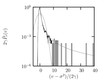
Figure 5: Probability density function for the random error in the estimated residual variance. Results shown are for a kernel estimate of the PDF resulting from $10^{4}$ estimates with $r=10^{3}$ for each estimate (black). Grey lines show the predicted large $r$ limit (a Stable PDF). For comparison, a Normal distribution with a mean and variance taken to be the sample mean and variance of the data is also shown (dotted line).

Figure 5 shows the general form of the distribution in the limit of large $r$, together with a kernel estimate of the same distribution constructed from $10^{4}$ residual variance estimates, each from $r=10^{3}$ local energy samples for the all-electron carbon atom considered for total energy estimates. For comparison, a Normal distribution resulting from blindly applying the CLT using the mean and variance of the sampled data is also shown. It is clear that the distribution of estimated residual variance is far from Normal, and it should be remembered that the width of the Normal distribution (in units of $2\gamma$) shown in the figure diverges with increasing number of residual variance estimates.

Observing that the limiting distribution describes the carbon data well, and that $r=10^{3}$ is a relatively small number of sample points, suggests that the large $r$ limit has been reached in this case. For less accurate trial wavefunctions this may not be the case. Since the deviation from the large $r$ limit has a magnitude proportional to $r^{-1/3}$ this should be justified on a case by case basis.

The significance of the deviation from the Normal distribution may best be estimated by considering the predicted number of estimates in the interval $(v-\sigma^{2})/2\gamma>2$, for $10^{4}$ estimates. Incorrectly assuming the validity of the CLT predicts $0.0$ outliers, Eq. (70) (with $\lambda_{3}=1.0$) predicts $\sim 266$ outliers, whereas the numerical data provides $198$ estimates in this interval. Confidence intervals could be defined using Eq. (70) and estimates of the parameter $\lambda_{3}$. This is not carried out here. A variety of methods for the estimation of parameters such as $\lambda_{3}$ do exist, but are inherently biasednolan01 .

It appears that the most important non-Gaussian features of the distribution of sample residual variance estimates are that $\gamma\propto r^{-1/3}$, and that outliers are likely.

Results for the estimate of both the total energy and the residual variance may be summarised in the statement that the ‘standard sampling’ method does not sample the $E^{-4}$ tails sufficiently to provide a statistically accurate measure of their contribution to estimates. Were these leptokurtotic tails to be absent, none of the deficiencies described above would be present - all moments of the local energy distribution would exist, leptokurtotic tails could not occur, and unbiased estimates that include finite sample size effects would be readily available.

These results do not invalidate the current use of ‘standard sampling’ for total energy or variance estimates, since these estimates still converge to the expectation values for increasing $r$. The difficulty is that estimates of the random error in these quantities are not available. It may be that assuming ‘$r$ is large enough’ provides practical estimates of the error in the total energies estimates, but whether this is the case depends on more than the sample moments. Errors in the residual variance estimates are unavoidably not Normal, even in the large $r$ limit, and the probability of outliers occurring does not fall off exponentially with $r$, but as a power law.

Estimated total energies and residual variance were chosen for consideration because of the central role played by these quantities in QMC methods. In the next section the results of a similar analysis of the ‘standard sampling’ estimates for other physical quantities is described, to show that the emergence of a non-Normal distribution of errors with power law tails is not limited to estimates of the residual variance.

IV Other Estimates

The analysis given in the preceding sections can be applied to general estimates in ‘standard sampling’ VMC to obtain the distribution of the accompanying random error. Ideally, it would be hoped that accurate confidence limits would be available as a result of the CLT being valid in its strongest form.

In this section estimates of the expectation value of several operators are considered, and these take the general form

$$\mathsf{A}_{r}\left[X\right]=\frac{1}{r}\sum_{n=1}^{r}x_{L}(\text{R}_{n}),$$ (73)

a mean of a local quantity $x_{L}$. Singularities in $x_{L}$ can be classified by location as type 1,2, or 3 in the same manner as for the local energy singularities, but the order of the singularities is generally different. The distribution of the estimates themselves are then obtained via the same surface integration and generalised central limit theorem approach used for the local energy.

IV.1 Kinetic energy and Potential energy

The most straightforward estimate for the electronic kinetic energy is provided by the kinetic part of the local energy,

$$x_{L}(\text{R}_{n})=\left[-\frac{1}{2}\frac{\nabla^{2}_{\mathbf{R}}\psi}{\psi}\right]_{\text{R}_{n}}.$$ (74)

This possesses type 1 and 2 singularities if the Kato cusp conditions are satisfied, and type 3 singularities unless $\nabla^{2}_{\mathbf{R}}\psi=0$ at the nodal surface. These singularities result in a Normal distribution of estimates in the large $r$ limit, with ‘lopsided’ $x^{-4}$ tails in the PDF that decay with increasing $r$. However, the presence of type 1 and 2 singularities is expected to result in larger $x^{-4}$ tails in the PDF of the kinetic energy estimate than for the total energy estimate.

An alternative estimator for the kinetic energy is provided via Green’s $1^{st}$ theorem, and takes the form of the sample average of the random variable

$$x_{L}(\text{R}_{n})=\frac{1}{2}\left[\sum_{i}\frac{\nabla_{i}\psi\cdot\nabla_{i}\psi}{\psi^{2}}\right]_{\text{R}_{n}},$$ (75)

where $\nabla_{i}$ denotes the gradient with respect to the co-ordinate of electron $i$. Type 1 and 2 singularities are not present since the gradient of the wavefunction possesses no singularities. Type 3 singularities arise from the quadratic behaviour of $\psi^{2}$ about the nodal surface, resulting in a positive $x^{-5/2}$ tail in the PDF of the sampled random variable and no CLT. The resulting PDF of kinetic energy estimates is the same one sided Stable PDF as for the residual variance estimates, with infinite variance and a $x^{-5/2}$ power law tail.

Two potential energy estimates follow naturally from the two kinetic energy estimates and the total energy estimate. One of these possesses type 1 and 2 singularities, and results in a weakly valid CLT with strong $x^{-4}$ tails. The second possesses type 3 singularities only, which result in no valid CLT, and the same one sided Stable PDF as the residual variance estimate, with infinite variance and a $x^{-5/2}$ power law tail.

IV.2 Non-local Pseudopotentials

For systems described using non-local pseudopotentials, the local energy estimate takes the form

$$x_{L}(\text{R}_{n})=\left[T_{L}+V_{ee}+\psi^{-1}\hat{V}\psi\right]_{\text{R}_{n}},$$ (76)

where $\hat{V}$ is the sum of one-body non-local operators that make up the pseudopotential. Provided the pseudopotential is not singular these do not possess type 1 singularities, and type 2 singularities may be prevented using the usual Kato cusp conditions. However, strong type 3 singularities can be expected at the nodal surface, resulting in $x^{-4}$ tails in the sample PDF. Hence, for non-local pseudopotentials, the CLT is expected to be weakly valid, with slowly decaying $x^{-4}$ tails that are larger than for the local potential case.

IV.3 Mass polarisation and relativistic terms

Corrections to the total energy due to finite nucleus mass and some relativistic effects may be implemented in VMC via perturbation theory, and the required estimates are available in the literaturekenny95 ; vrbik88 . These generally possess singularities of all three types, and result in $x^{-5/2}$ tails in the PDF of the sampled local variable. As a direct consequence of these tails the CLT is not valid and the large sample size limit of the distribution of estimates is not Normal, but a two sided variant of the Stable PDF found for the residual variance estimate, that is with a finite mean, an infinite variance, and two sided $x^{-5/2}$ power law tails.

IV.4 Atomic force estimates

For estimates of atomic forces the ‘local Hellmann-Feynman force’ is commonly taken to possess the formbadinski07

$$x_{L}(\text{R}_{n})=-\left[\nabla_{\mathbf{X}}\left(\psi^{-1}\hat{V}\psi\right)\right]_{\text{R}_{n}},$$ (77)

where $\nabla_{\mathbf{X}}$ is the gradient with respect to the nucleus co-ordinate(s), $\mathbf{X}$, evaluated at the nucleus positions of interest, and $\hat{V}$ is the sum of one-body potential energy operators due to each atomic nucleus in the system. (Both the operator and the trial wavefunction are functions of the nucleus position.)

For the special case where $\hat{V}$ is a local potential the wavefunction cancels, and the gradient operator acts on the multiplicative potential only. For smooth local potentials no singularities arise, and the CLT is valid for the resulting estimate. For a Coulomb potential type 1 singularities arise, and result in estimates whose distribution in the large sample size limit is a two sided Stable law of finite mean, infinite variance, and with $x^{-5/2}$ power law tails. For smooth non-local pseudopotentials type 3 singularities arise, and result in estimates whose distribution in the large sample size limit is, again, a two sided Stable law with $x^{-5/2}$ power law tails.

IV.5 Linearised basis optimisation

A wavefunction optimisation strategy has recently been developedumrigar07 ; brown07 that linearises the influence of variational parameters on the total energy by constructing a basis set from derivatives of the trial wavefunction with respect to parameters of the wavefunction, $\alpha_{i}$. Applying the total energy variational principle results in a matrix diagonalisation problem, with matrix elements defined by integrals that are estimated as means of the sample values

$$x_{L}(\text{R}_{n})=\left[\frac{\psi_{i}}{\psi}\frac{\hat{A}\psi_{j}}{\psi}\right]_{\text{R}_{n}},$$ (78)

with $\psi_{i}$ the derivative of the trial wavefunction with respect to parameters $\alpha_{i}$, except for $\psi_{0}=\psi$. $\hat{A}$ is either the identity or the Hamiltonian operator.

Generally, the linear behaviour of the wavefunction as the nodal surface is crossed introduces singularities in the sampled quantity, resulting in $x^{-5/2}$ tails in the PDF. These result in an invalid CLT, and the estimated matrix elements have a PDF (in the large sample size limit) of the same form as for the estimate of the residual variance - the one sided Stable distribution with infinite variance. Some exceptions occur for particular matrix elements; for the Hamiltonian operator the distribution of the estimate is weakly Normal for $i=0$, and for the identity operator the CLT is weakly valid for $i=0$ or $j=0$, and the variance is zero for $i=j=0$.

Although this informs us of the distribution of each estimated matrix element, it provides no direct information on the correlation between elements, or of the distribution of the lowest eigenvalue of the estimated matrixedelman91 . However, it seems likely that the invalidity of the CLT makes a significant contribution to the instabilities that must be carefully controlled for an implementation of this optimisation method to be successful.

V Conclusion

The sampling distribution for a local quantity can be simplified by reducing the $3N$-dimensional distribution to the degrees of freedom of the local quantity that is sampled, with derivable asymptotic behaviour. Such an analysis has been applied here to characterise the random error for the two most important estimated quantities in variational QMC, the total energy and the residual variance.

For estimates of the total energy within the ‘standard sampling’ implementation of VMC, the CLT is found to be valid in its weakest form with the consequence that the influence of finite sample size is not obvious and must be considered on a case by case basis. Outliers have been found to be significantly more likely than suggested by CLT confidence limits. No rigorous bounds exist that provide limits to the deviation from the CLT for finite $r$, and consequently confidence intervals based on the CLT may be misleading. However, for the example case of an all-electron isolated carbon atom and an accurate trial wavefunction the assumption of large sample size appears to be useful.

The variance of the local energy has also been considered in light of the primary role played by this and similar quantities in wavefunction optimisation procedures. A statistical variance of the local energy within ‘standard sampling’ is equivalent to the residual variance defined in terms of the Hamiltonian and trial wavefunction themselves, and the statistics of the estimate of this quantity have been investigated.

For estimates of the variance within the ‘standard sampling’ implementation the CLT is found to be invalid. A more general Stable distribution and generalised central limit theorem take the place of the Normal distribution and CLT, and this Stable distribution is fundamentally different from the Normal distribution. It possesses tails that decay algebraically, and so outliers are many orders of magnitude more likely than suggested by the CLT. The width scale of this distribution falls as $r^{-1/3}$, significantly slower than the $r^{-1/2}$ scaling that would result from a valid CLT. The distribution is asymmetric, so the mean and mode do not coincide. Only biased estimates of the parameters of this distribution (other than its mean) are available, and confidence intervals based on the CLT are entirely invalid.

In order to demonstrate that this is not a statistical issue particular to estimating the residual variance, estimates of the expectation values of several other operators have also been considered. For most of these the CLT is found to be invalid, with the same or a similar distribution of random error arising as for the residual sampling estimate - the Stable distribution with $x^{-5/2}$ asymptotic tails and infinite variance.

Perhaps the most important consequence of these results arises in the context of the minimisation of the residual variance and related quantities carried out to optimise a trial wavefunction. Many of the instabilities encountered in different optimisation methodskent99 ; bressanini02 may be due to the use of estimates that are statistically faulty.

By shedding an assumption about the properties of QMC estimates and replacing this with a derivation of the true distribution of random errors, it has been shown that deviations from the CLT are not trivial and can be expected to have a significant influence on the accuracy and reliability of estimated physical quantities and optimisation strategies within QMC. The analysis itself provides a new explicit (but not rigorously closed) expression for a particular Stable law PDF, and a general approach to assessing the strengths and failures of general sampling strategy/trial wavefunction combinations for estimating expectation values of physical quantities in QMC.

*

Appendix A

Defining $a^{3/2}=\frac{4\lambda_{3}}{3\sqrt{\pi}}$ gives $\chi_{0}$ of Eq. (67) as

$$\chi_{0}(v)=\frac{1}{2\pi}\int_{-\infty}^{\infty}\exp\left[-a^{3/2}\left(1-i\;\textrm{sgn}[w]\right)|w|^{3/2}\right]e^{iwv}dw.$$ (79)

Partitioning the integral into the negative and positive ranges gives

$$\chi_{0}(v)=I_{1}(v)+I_{2}(v),$$ (80)

with $I_{1}$ and $I_{2}$ integrals taken over $0\leq w<\infty$ and $-\infty<w<0$, respectively. Substituting $w=y^{2}$ results in

$$I_{1}(v) = \frac{1}{2\pi}\int_{0}^{\infty}2y\exp\left[ivy^{2}-a^{3/2}(1-i)y^{3}\right]dy,$$

and, for $I_{2}$, substituting $w=-y^{2}$ results in

$$I_{2}(v) = \frac{1}{2\pi}\int_{0}^{\infty}2y\exp\left[-ivy^{2}-a^{3/2}(1+i)y^{3}\right]dy$$ (82)

$$= I_{1}(v)^{*}.$$

These two identities provide

$$\chi_{0}(v) = I_{1}(v)+I_{1}(v)^{*}$$

$$= \frac{1}{\pi}\Re\left[\int_{0}^{\infty}2y\exp\left[ivy^{2}-a^{3/2}(1-i)y^{3}\right]dy\right].$$

The next step is to obtain the real part of the integral in this expression. This can be achieved by converting this integral into an ODE for $\chi_{0}(v)$, and then seeking the solutions that are real and normalised.

First define $G_{n}$ by

$$G_{n}(v)=\int_{0}^{\infty}2y^{n}\exp\left[ivy^{2}-a^{3/2}(1-i)y^{3}\right]dy,$$ (84)

so that

$$\chi_{0}(v)=\frac{1}{\pi}\Re\left[G_{1}(v)\right].$$ (85)

Equations that relate $G_{n}$ for different indices may be derived. The first of these is obtained by integrating the derivative of the exponential function in the integrand to give

$$\int_{0}^{\infty}\left(2ivy-3a^{3/2}(1-i)y^{2}\right)\exp\left[ivy^{2}-a^{3/2}(1-i)y^{3}\right]dy=\left.\exp\left[ivy^{2}-a^{3/2}(1-i)y^{3}\right]\right|_{v=0}^{v=\infty}.$$ (86)

In addition integrating $G_{n}$ by parts provides the relation

$$(n+1)G_{n}=-2ivG_{n+2}+3a^{3/2}(1-i)G_{n+3}.$$ (87)

These two expressions provide the equations

$$-1 = \;\;\;ivG_{1}-\frac{3}{2}a^{3/2}(1-i)G_{2}$$ (88)

$$G_{1} = -ivG_{3}-\frac{3}{2}a^{3/2}(1-i)G_{4}$$ (89)

$$G_{2} = -\frac{2}{3}ivG_{4}+a^{3/2}(1-i)G_{5},$$ (90)

where the first arises from evaluating the limits in Eq. (86) explicitly and expressing the LHS in terms of $G_{1}$ and $G_{2}$ and the following two arise from Eq. (87) for $n=1,2$.

Combining these equations to remove $G_{2}$ and $G_{4}$, and noting that $\frac{dG_{1}}{dv}=iG_{3}(v)$ and $\frac{d^{2}G_{1}}{dv^{2}}=-G_{5}(v)$ provides

$$9a^{3}G_{1}^{\prime\prime}-2v^{2}G_{1}^{\prime}-5vG_{1}=-3i.$$ (91)

Making the substitutions

$$G_{1}(v)=v^{2}e^{\left(\frac{v}{3a}\right)^{3}}g(v)$$ (92)

and

$$x=\left(\frac{v}{3a}\right)^{3},$$ (93)

further simplifies this ODE, and results in the inhomogeneous ODE

$$x^{2}g^{\prime\prime}+2xg^{\prime}-\left(x^{2}+x-\frac{2}{9}\right)g=-\frac{1}{27a^{3}}ie^{-x}.$$ (94)

Only the real solutions of this equations are required, hence only the homogeneous ODE

$$x^{2}g^{\prime\prime}+2xg^{\prime}-\left(x^{2}+x-\frac{2}{9}\right)g=0$$ (95)

need be considered. The required solution is finite for $x\rightarrow\pm\infty$ and continuous at $x=0$, and is a sum of two modified Bessel functions of the second kind,

$$g(x)=A\left[-\textrm{sgn}(x)K_{1/3}\left(\left|x\right|\right)+K_{2/3}\left(\left|x\right|\right)\right],$$ (96)

with $A$ an undefined constant.

Requiring Eq. (88) to be true for $v=0$ provides $A$, and transforming back to $v$ provides the final result

$$\chi_{0}(v)=\frac{\sqrt{3}}{\pi}\frac{v^{2}}{(3a)^{3}}e^{(v/(3a))^{3}}\left[-\textrm{sgn}(v)K_{1/3}\left(\left|\frac{v}{3a}\right|^{3}\right)+K_{2/3}\left(\left|\frac{v}{3a}\right|^{3}\right)\right].$$ (97)

The transformation between $v$ and a more general variable is described in the main text.

This provides an explicit form for the PDF of the Stable distribution ${\bf S}\left(3/2,-1,\gamma,\delta;1\right)$ (using the notation of Nolannolan01 ) - Eq. (97) is for $(\gamma,\delta)=(a,0)$ and the general form is trivially related to this by rescaling and translation.

References

- (1) W. M. C. Foulkes, L. Mitas, R. J. Needs, and G. Rajagopal, Rev. Mod. Phys. 73, 33 (2001).
- (2) J. F. Traub and A. G. Wershulz, Complexity and Information (Cambridge University Press, 1998).
- (3) R. Assaraf and M. Caffarel, J. Chem. Phys. 119, 10536 (2003); R. Assaraf, M. Caffarel, and A. Scemama, Phys. Rev. A 75, 035701 (2007); J. Toulouse, R. Assaraf, and C. J. Umrigar, J. Chem. Phys. 126, 244112 (2007).
- (4) J. R. Trail, Phys. Rev. E 77, 016704 (2008).
- (5) D. W. Stroock, Probability Theory: An analytic view (Cambridge University Press, 1993).
- (6) R. T. Pack and W. B. Brown, J. Chem. Phys. 45, 556 (1966).
- (7) C. R. Myers, C. J. Umrigar, J. P. Sethna, and J. D. Morgan III, Phys. Rev. A 44, 5537 (1991).
- (8) M. Bajdich, L. Mitas, G. Drobny, and L. K. Wagner, Phys. Rev. B 72, 075131 (2005).
- (9) C. F. Fischer, G. Tachiev, G. Gaigalas, and M. Godefroid, Comput. Phys. Commun. 176, 559 (2007) (http://atoms.vuse.vanderbilt.edu).
- (10) N. D. Drummond, M. D. Towler, and R. J. Needs, Phys. Rev. B 70, 235119 (2004).
- (11) P. López Ríos, A. Ma, N. D. Drummond, M. D. Towler, and R. J. Needs, Phys. Rev. E 74, 066701 (2006).
- (12) R. J. Needs, M. D. Towler, N. D. Drummond and P. López Ríos, CASINO user’s guide, version 2.0.0 (2006).
- (13) S. J. Chakravorty, S. R. Gwaltney, E. R. Davidson, F. A. Parpia, and C. F. Fischer, Phys. Rev. A 47, 3649 (1993).
- (14) A. J. Izenman, J. Am. Stat. Assoc. 86, 204 (1991).
- (15) D. Bressanini, G. Morosi, and M. Mella, J. Chem. Phys. 116, 5345 (2002).
- (16) P. R. C. Kent, R. J. Needs, and G. Rajagopal, Phys. Rev. B 59, 12344 (1999).
- (17) R. Bianchi, P. Cremaschi, G. Morosi, and C. Puppi, Chem. Phys. Lett. 148, 86 (1988).
- (18) V. R. Pandharipande, S. C. Pieper, and R. B. Wiringa, Phys. Rev. B 34, 4571 (1986).
- (19) , in Normal Approximation: New Results, Methods and Problems (VSP International Science, Leiden, The Netherlands, 1998).
- (20) B. V. Gnedenko and A. N. Kolomogorov, Limit Distributions for Sums of Independent Random Variables (Addison-Wesley, 1968).
- (21) P. M. Morse and H. Feshbach, Methods of Theoretical Physics, (McGraw Hill, 1953).
- (22) S. A. Alexander, R. L. Coldwell, H. J. Monkhorst, and J. D. Morgan III, J. Chem. Phys. 86, 6622 (1991).
- (23) H. Conroy, J. Chem. Phys. 41, 1331 (1964).
- (24) J. P. Nolan, in Stable Distributions - Models for Heavy Tailed Data, (Birkhauser, Boston 2001).
- (25) S. D. Kenny, G. Rajagopal, and R. J. Needs, Phys. Rev. A 51, 1898 (1995).
- (26) J. Vrbik, M. F. DePasquale, and S. M. Rothstein, J. Chem. Phys. 88, 3784 (1988).
- (27) A. Badinski and R. J. Needs, Phys. Rev. E 76, 036707 (2007).
- (28) C. J. Umrigar, J. Toulouse, C. Filippi, S. Sorella, and R. G. Hennig, Phys. Rev. Lett. 98, 110201 (2007).
- (29) M. D. Brown, J. R. Trail, P. Lopez Rios, and R. J. Needs, J. Chem. Phys., J. Chem. Phys. 126, 224110 (2007).
- (30) A. Edelman, Linear Algebra and its Applications 159, 55 (1991).