nuclear interactions
and the space-like structure of the pion

Abstract:

Three instances are discussed in which results produced by chiral perturbation theory can be reliably pushed to high space-like values of transferred momenta.
1. nuclear interactions:   At present, expansions are available for about 20 components of both two- and three-nucleon forces, and the vast majority of them follows the patterns predicted by chiral symmetry. The outstanding exception is $V_{C}^{+}$, the isospin independent central potential. Standard calculations show that this ${\cal{O}}(q^{3})$ contribution is about 10 times larger than the leading ${\cal{O}}(q^{2})$ isospin dependent term $V_{C}^{-}$. In spite of defying counting rules, these results are quite well supported by phenomenology up to distances smaller than 1 fm $(\rightarrow|t|\sim 20\;M_{\pi}^{2})$.
2. nucleon sigma-term:   The configuration space nucleon scalar form factor $\tilde{F}_{s}(r)$ is an important substructure of $V_{C}^{+}$, and its integration over the entire volume yields $\sigma_{N}$, the nucleon $\sigma$-term. Perturbative results based on diagrams involving $N$ and $\Delta$ intermediate states vanish at large distances, and increase monotonically as one approaches the nucleon center, where they can become arbitrarily large. Assuming that the pion cloud of the nucleon is constructed at the expenses of the surrounding condensate, an upper limit for $\tilde{F}_{S}(r)$ can be set at a critical radius $R\simeq 0.6$ fm $(\rightarrow|t|\sim 40\;M_{\pi}^{2})$, where a phase transition takes place. This mechanism excludes the problematic region and yields 43 MeV$<\sigma_{N}<\;$49 MeV, in agreement with the empirical value 45$\pm 8$ MeV.
3. space-like structure of the pion:   The extension of the model for $\sigma_{N}$ to the pion describes it as a Goldstone boson at large distances, surrounded by a quark-antiquark condensate. As one moves towards its center, the condensate is gradually destroyed and a phase transition occurs at a distance $R\simeq 0.6$ fm $(\rightarrow|t|\sim 40\;M_{\pi}^{2})$. When only pion loops are considered, the model depends on just $M_{\pi}$ and $F_{\pi}$, and yields $\langle\;r^{2}\;\rangle_{S}^{\pi}=0.50$ fm² and $\bar{l}_{4}=3.9$. The inclusion of a scalar resonance of mass $980\,$MeV, with two known coupling constants, improves these values to $\langle\;r^{2}\;\rangle_{S}^{\pi}=0.59$ fm² and $\bar{l}_{4}=4.3$, well within the error bars of the precise estimates $\langle\;r^{2}\;\rangle_{S}^{\pi}=0.61\pm 0.04$ fm² and $\bar{l}_{4}=4.4\pm 0.2$, produced in 2001 by Colangelo, Gasser and Leutwyler. In both cases, results are given in terms of simple analytic expressions.

1 NUCLEAR INTERACTIONS

In the last twenty years, our understanding of nuclear interactions has improved considerably[1], owing to the systematic use of chiral perturbation theory (ChPT)[2]. As the masses of the quarks $u$ and $d$ are small, they are treated as perturbations in a $SU(2)\times SU(2)$ chiral symmetric lagrangian. Hadronic amplitudes are then expanded in terms of a typical scale $q$, set by either pion four-momenta or nucleon three-momenta, such that $q\ll 1$ GeV. This procedure is rigorous and results are written as power series in the scale $q$, giving rise to the notion of chiral hierearchies. In most cases, leading order terms come from tree diagrams and corrections require the inclusion of pion loops.

In spite of all the progress achieved, there are still some puzzles in our picture of nuclear interactions. At present, chiral symmetry has been applied to about 20 components of nuclear forces[3], and the predicted structure for the most important terms is shown in table 1, where $OPE$and $TPE$ stand for one-pion exchange and two-pion exhange, $V_{i}^{+}$ and $V_{i}^{-}$ represent two-body operators proportional to either the identity or $\mbox{\boldmath$\tau$}^{(1)}\!\cdot\!\mbox{\boldmath$\tau$}^{(2)}$ in isospin space, $i\rightarrow$ [central$(C)$, spin-orbit$(LS)$, spin-spin$(SS)$, tensor$(T)$], whereas the notation of ref.[4] is used for three-body forces. Actual results for central components $V_{C}^{\pm}$ defy these predictions.

leading	TWO-BODY	TWO-BODY	THREE-BODY
contribution	$OPE$	$TPE$	$TPE$
${\cal{O}}(q^{0})$	$V_{T}^{-},V_{SS}^{-}$
${\cal{O}}(q^{2})$		$V_{C}^{-};V_{T}^{+},V_{SS}^{+}$
${\cal{O}}(q^{3})$		$V_{LS}^{-},V_{T}^{-},V_{SS}^{-};V_{C}^{+},V_{LS}^{+}$	$W_{S},W_{P},W_{P}^{\prime}$

The chiral two-pion exchange $NN$ potential was studied by our group[5, 6], by means of the three families of diagrams displayed in fig.1. Family $I$ implements the minimal realization of chiral symmetry[7] and begins at ${\cal{O}}(q^{2})$, whereas family $I\!I$ depends on $\pi\pi$ correlations and contributes at ${\cal{O}}(q^{4})$. Vertices in these familes involve only $g_{A}$ and $F_{\pi}$, and all dependence on other LECs is concentrated in family $I\!I\!I$, which begins at ${\cal{O}}(q^{3})$. These LECs can be extracted from subthreshold $\pi N$ amplitudes[8] and one finds that the components $V_{C}^{-}$ and $V_{C}^{+}$ are very strongly dominated by families $I$ and $I\!I\!I$, respectively.

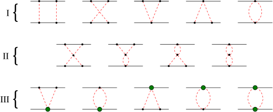
Figure 1: Dynamical structure of the two-pion exchange potential.

The central components $V_{C}^{-}[\rightarrow{\cal{O}}(q^{2})]$ and $V_{C}^{+}[\rightarrow{\cal{O}}(q^{3})]$ are shown in fig.2, and one has $|V_{C}^{+}|\sim 10\,|V_{C}^{-}|$ in regions of physical interest, at odds with the predicted chiral hierarchy. The numerical explanation for the magnitude of $V_{C}^{+}$ is that it depends on large LECs generated by delta intermediate states. Nevertheless, the prediction for $V_{C}^{+}$, which is by far the most important component of the nuclear force, is very good when compared with accurate phenomenological Argonne[9] potentials. Moreover, this agreement holds up to distances smaller than 1 fm, which correspond to momenta transferred $|t|>20\,M_{\pi}^{2}$. The empirical validity of results for $V_{C}^{+}$ is, thus, much wider than expectations allowed by chiral perturbation theory.

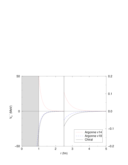
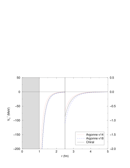
Figure 2: Isospin odd (left) and even (right) central components of the two-pion exchange potential.

2 NUCLEON SIGMA-TERM

The structure of $V_{C}^{+}$ was discussed in refs.[6, 10], and about $70\%$ of its strength found to come from a term of the form

$$V_{C}^{+}(r)\sim-\,(2\,c_{3}/F_{\pi}^{2})\;\left[2-4c_{1}/c_{3}-\mbox{\boldmath$\nabla$}^{2}/M_{\pi}^{2}\right]\;\tilde{\sigma}_{N}(r)\;,$$ (1)

where $\tilde{\sigma}_{N}$ is the long-distance part of the scalar form factor in configuration space and the $c_{i}$ are usual LECs from the $\pi N$ lagrangian. An important role is played by $c_{3}$, which is large and dominated by $\Delta$ intermediate states.

The nucleon scalar form factor is defined in terms of the symmetry breaking lagrangian as

$$\langle\;N(p^{\prime})|\!-\!{\cal{L}}_{sb}\,|N(p)\;\rangle=\bar{u}(p^{\prime})\;u(p)\;\sigma_{N}(t)\;.$$ (2)

and has already been expanded to ${\cal{O}}(q^{4})$[11, 8]. The leading ${\cal{O}}(q^{2})$ contribution comes from a tree diagram proportional to $c_{1}$, whereas corrections at ${\cal{O}}(q^{3})$ and ${\cal{O}}(q^{4})$ are due to loops involving nucleon intermediate states and LECs. The main features of these results were incorporated into a model for the scalar form factor in configuration space[12], in which LECs at ${\cal{O}}(q^{4})$ are replaced by explicit $\Delta$ intermediate states. The corresponding structure reads

$$\tilde{\sigma}_{N}(\mbox{\boldmath$r$}) \!=\! \left[-4\,c_{1}\,\mu^{2}\,\delta^{3}(\mbox{\boldmath$r$})\;\right]_{{\cal{O}}(q^{2})}\;+\;\left[\;\tilde{\sigma}_{N}(r)\;\right]_{{\cal{O}}(q^{3})}^{N}\;+\;\left[\;\tilde{\sigma}_{N}(r)\;\right]_{{\cal{O}}(q^{4})}^{\Delta}\;,$$ (3)

the superscripts $N$ and $\Delta$ indicating intermediate propagators in triangle diagrams. These contributions are first evaluated in momentum space, by using ${\cal{L}}_{sb}=F_{\pi}^{2}\,M_{\pi}^{2}\,\cos\theta$, where $\theta$ is the pion field, related to the usual unitary form by $U=\exp(i\mbox{\boldmath$\tau$}\cdot\mbox{\boldmath$\theta$})=\cos\theta+i\mbox{\boldmath$\tau$}\cdot\hat{\mbox{\boldmath$\theta$}}\,\sin\theta$. Results are then expressed as $\sigma_{N}(t)=-F_{\pi}^{2}\,M_{\pi}^{2}\;\cos\theta(t)$.

Performing a Fourier transform and recalling that the vacuum expectation value of ${\cal{L}}_{sb}$ is related to the light quark condensate by $\langle\;0|-{\cal{L}}_{sb}\,|0\;\rangle=\langle\;0|\hat{m}(\bar{u}u+\bar{d}d)|0\;\rangle=-\,F_{\pi}^{2}\,M_{\pi}^{2}$, the scalar form factor in coordinate space is written as

$$\check{\sigma}_{N}(r)=\langle\;0|\hat{m}(\bar{u}u+\bar{d}d)|0\;\rangle\;\cos\theta(r)\;.$$ (4)

The function $\cos\theta(r)$ describes the disturbance produced by the nucleon over the condensate and the non-linear nature of pion interactions gives rise to the constraint

$$-1\leq\check{\sigma}_{N}(r)/\langle\;0|\hat{m}(\bar{u}u+\bar{d}d)|0\;\rangle\leq 1\;.$$ (5)

Another condition over this ratio comes from the fact that the QCD ground state can take the form of either empty space or a quark-antiquark condensate. In the present case, the boundary condition $\theta(r)\rightarrow 0$ for $r\rightarrow\infty$ ensures that the condensate remains undisturbed at large distances. As one moves towards the nucleon, $\cos\theta$ decreases, indicating that it destroys the condensate. This picture is compatible with the unitarity of the field $U$, which correlates condensate and pion magnitudes and suggests that the pion cloud of the nucleon is constructed at the expenses of the surrounding condensate, by means of a chiral rotation. The model presented in ref.[12] is based on the assumption that this process ends when all quark-antiquark pairs originally present in the vacuum become excited, and a phase transition takes place at the radius $R$ at which $\cos\theta(R)=0$. Formally, this corresponds to the condition

$$0\leq\check{\sigma}_{N}(r)/\langle\;0|\hat{m}(\bar{u}u+\bar{d}d)|0\;\rangle\leq 1\;.$$ (6)

In configuration space, observables are calculated by integrating densities over the entire volume. In the case of the density $\check{\sigma}_{N}$, given by eq.(4), this would yield divergent results, since it does not vanish in the limit $r\rightarrow\infty$. Therefore one shifts its origin, and works with a new function, defined as

$$\tilde{\sigma}_{N}(r)\equiv\check{\sigma}_{N}(r)-\langle\;0|\hat{m}(\bar{u}u+\bar{d}d)|0\;\rangle=F_{\pi}^{2}\,M_{\pi}^{2}\;\left[1-\cos\theta(r)\right]\;,$$ (7)

which describes the nucleon cloud as a deviation from the condensate. In practice, the function $\cos\theta$ cannot be calculated exactly and one resorts to perturbation. This naturally yields a representation for $[1-\cos\theta]$ which vanishes at large distances and increases monotonically as one approaches the nucleon center. At short distances, this representation becomes inadequate, since it is unbound and diverges at the origin. In the model, this problematic region is excluded by the phase transition, for it assumes the perturbative representation for $\cos\theta$ in the range $R\leq r<\infty$ and $\cos\theta=0$ for $R<r$.

The roles played by $N[\rightarrow{\cal{O}}(q^{3})]$ and $\Delta[\rightarrow{\cal{O}}(q^{4})]$ intermediate states in eq.(3) can be inferred from fig.3. The ratio $\left[\;\tilde{\sigma}_{N}(r)\;\right]^{N}/\left[\;\tilde{\sigma}_{N}(r)\;\right]^{\Delta}$, given on the left, shows that the hierarchy predicted by ChPT breaks down for distances smaller than 1.5 fm. The right figure describes the ratio $\tilde{\sigma}_{N}(r)/(F_{\pi}^{2}\,M_{\pi}^{2})=(1-\cos\theta)$ inside this region, together with individual $N$ and $\Delta$ contributions. The phase transition is assumed to occur at the point $R\sim 0.6$ fm $(\rightarrow|t|\sim 40\,M_{\pi}^{2})$, where the black curve reaches the value 1.

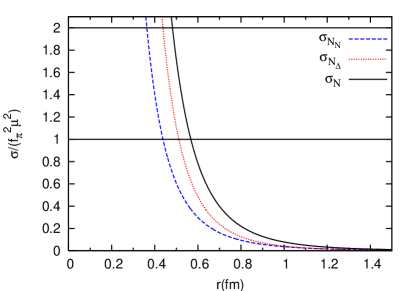
Figure 3: Ratios $[\tilde{\sigma}_{N}(r)]^{\Delta}/[\tilde{\sigma}_{N}(r)]^{N}$ (left) and $\tilde{\sigma}_{N}(r)/(F_{\pi}^{2}\,M_{\pi}^{2})=(1-\cos\theta)$ (right) as functions of the distance to the nucleon center.

In ref. [12], the nucleon $\sigma$-term has been evaluated by means of the expression

$$\sigma_{N}=\frac{4}{3}\pi R^{3}\;F_{\pi}^{2}M_{\pi}^{2}+4\pi\int_{R}^{\infty}dr\;r^{2}\;\tilde{\sigma}_{N}(r)\;,$$ (8)

which yields 43 MeV$<\sigma_{N}<\;$49 MeV, depending on the value used for the $\pi N\Delta$ coupling constant, in agreement with the empirical value 45$\pm 8$ MeV [13]. Good results are also obtained for the $\Delta$ $\sigma$-term.

3 SPACE-LIKE STRUCTURE OF THE PION

Configuration space results for $V_{C}^{+}$ and $\sigma_{N}$ indicate that, in these two instances, perturbative calculations are reliable at high values of $|t|$. This has motivated an exploratory study of pion properties in a similar framework[14], which yields good predictions for the mean square radius $(\langle\;r^{2}\;\rangle_{S}^{\pi}=0.59\,$fm${}^{2})$ and for one of the LECs $(\bar{l}_{4}=4.3)$, with no free parameters.

The calculation departs from standard ${\cal{O}}(q^{4})$ results produced by Gasser and Leutwyler (GL) in 1984[15], and their notation is followed. The pion scalar form factor is given by

$$F_{S}(t) \!=\! \langle\;\pi(\mbox{\boldmath$p$}^{\prime})\,|\,\bar{u}\,u+\bar{d}\,d\;|\,\pi(\mbox{\boldmath$p$})\;\rangle=2B\,\left\{1+2\,\mu_{\pi}+\frac{M_{\pi}^{2}}{32\pi^{2}\,F_{\pi}^{2}}+\frac{4M_{\pi}^{2}}{F_{\pi}^{2}}\;l_{3}^{r}\right.$$ (9)

$$\!+\! \left.\frac{(2\,t-M_{\pi}^{2})}{32\pi^{2}\,F_{\pi}^{2}}\;L(M_{\pi},t)+\frac{t}{F_{\pi}^{2}}\,\left[l_{4}^{r}-\frac{1}{16\,\pi^{2}}\,\left(\ln\frac{M_{\pi}^{2}}{\mu^{2}}+1\right)\right]\right\}\;,$$

where $\mu_{\pi}=(M_{\pi}^{2}/32\pi^{2}F_{\pi}^{2})\ln(M_{\pi}^{2}/\mu^{2})$, the LECs are related to their scale-invariant counterparts by $l_{3}^{r}=-(\bar{l}_{3}+\ln M_{\pi}^{2}/\mu^{2})/64\pi^{2}$ and $l_{4}^{r}=(\bar{l}_{4}+\ln M_{\pi}^{2}/\mu^{2})/16\pi^{2}$, $t=(p^{\prime}-p)^{2}$, and the loop function $L$ is related to the $\bar{J}$ in GL by $\bar{J}=L/(4\pi)^{2}$. In the Breit frame, the variable $t=-q^{2}$ is negative and one has

$$L(M_{\pi},q)=\sigma\;\ln\frac{\sigma-1}{\sigma+1}+2\;,\hskip 14.22636pt\sigma=\sqrt{1+4\,M_{\pi}^{2}/q^{2}}\;.$$ (10)

The Fourier transform of $F_{S}(t)$ describes the spatial structure of the pion and reads

$$\tilde{F}_{S}(r) \!=\! 2B\;\left\{\frac{\tilde{\Lambda}(M_{\pi},r)}{32\pi^{2}F_{\pi}^{2}}+\mathrm{ZRT}\right\}\;,$$ (11)

$$\tilde{\Lambda}(M_{\pi},r) \!=\! \int\frac{d^{3}q}{(2\pi)^{3}}\;e^{-i\,\mbox{\boldmath$q$}\cdot\mbox{\boldmath$r$}}\;[(2t-M_{\pi}^{2})\,L(M_{\pi},q)]$$ (12)

$$\!=\! \frac{M_{\pi}^{3}}{\pi\,r^{2}}\,\left[\left(\frac{12}{M_{\pi}^{2}\,r^{2}}+7\right)\,K_{1}(2M_{\pi}r)+\frac{12}{M_{\pi}r}\;K_{0}(2M_{\pi}r)\right]\;,$$ (13)

where the $K_{i}$ are Bessel functions and ZRT stands for zero range terms, proportional to the $\delta$-function and its derivatives. The leading term in the quark condensate is given by $\langle\;0\,|\,\bar{u}\,u+\bar{d}\,d\,|\,0\,\;\rangle=-2B\,F_{\pi}^{2}$, and one writes

$$\tilde{F}_{S}(r)=-{\langle\;0\,|\,\bar{u}\,u+\bar{d}\,d\,|\,0\;\rangle}\;\frac{\tilde{\Lambda}(M_{\pi},r)}{32\pi^{2}F_{\pi}^{4}}+\mathrm{ZRT}\;.$$ (14)

At low-energies, the pion behaves as a Goldstone boson and, far away from its center, the scalar form factor must be related to the surrounding quark-antiquark condensate by $\tilde{F}_{S}(r)\rightarrow N\;\langle\;0\,|\,\bar{u}\,u+\bar{d}\,d\,|\,0\;\rangle$, where $N$ is a constant with dimension of mass. However, eq.(14) vanishes at large distances and, as in the case of eq.(7) for the nucleon, one has to perform a shift in the origin, defining a new function by

$$\check{F}_{S}(r)\equiv\tilde{F}_{S}(r)+\langle\;0|(\bar{u}u+\bar{d}d)|0\;\rangle=N\;\langle\;0\,|\,\bar{u}\,u+\bar{d}\,d\,|\,0\;\rangle\;\left[1-\,\frac{\tilde{\Lambda}(M_{\pi},r)}{N\,32\pi^{2}F_{\pi}^{4}}+\mathrm{ZRT}\right]\;.$$ (15)

This form is now suited for describing the behavior of the pion in the presence of the condensate. It is the analog to eq.(4), with $\cos\theta$ replaced by $[1-\,\tilde{\Lambda}(M_{\pi},r)/(N\,32\pi^{2}F_{\pi}^{4})+\mathrm{ZRT}]$. As in the nucleon case, it represents an undisturbed condensate at large distances and decreases monotonically as one approaches the center of the pion. For the same reasons as discussed in the previous section, one assumes that this term is meaningful in the interval

$$0\leq\left[1-\,\frac{\tilde{\Lambda}(M_{\pi},r)}{N\,32\pi^{2}F_{\pi}^{4}}+\mathrm{ZRT}\right]\leq 1\;,$$ (16)

and that a phase transition occurs at a point $R$, such that $1=\tilde{\Lambda}(M_{\pi},R)/(N\,32\pi^{2}F_{\pi}^{4})$. At smaller distances, the function $\tilde{\Lambda}(M_{\pi},r)$ is replaced by the cut version $\Theta(r-R)\,\tilde{\Lambda}(M_{\pi},r)$. Zero range terms are then eliminated and one has

$$\check{F}_{S}(r) \!=\! -\,2\,BF_{\pi}^{2}\,\left\{N-\Theta(r-R)\;\frac{\tilde{\Lambda}(M_{\pi},r)}{32\pi^{2}F_{\pi}^{4}}\right\}\;.$$ (17)

This function does not vanish at infinity and, as in the nucleon case, integration over entire space requires shifting the origin. The scalar form factor is then rewritten as

$$\tilde{F}_{S}(r)=2\,B\,\left\{\Theta(R-r)\;\frac{\tilde{\Lambda}(M_{\pi},R)}{32\pi^{2}F_{\pi}^{2}}+\Theta(r-R)\;\frac{\tilde{\Lambda}(M_{\pi},r)}{32\pi^{2}F_{\pi}^{2}}\right\}\;,$$ (18)

after using the cutting condition to eliminate the factor $N$.

The scalar form factor in momentum space is given by the Fourier transform of this result and, for $t=0$, one has $F_{S}(0)=4\pi\,\int dr\,r^{2}\tilde{F}_{S}(r)$. At leading order, eq.(9) yields $F_{S}(0)=2\,B$ and one has the consistency condition

$$1=4\pi\,\int dr\,r^{2}\;\frac{\tilde{F}_{S}(r)}{2B}=\frac{M_{\pi}^{2}}{16\pi^{2}F_{\pi}^{2}}\,\left[\left(\frac{20}{M_{\pi}R}+\frac{14\,M_{\pi}R}{3}\right)\,K_{1}(2M_{\pi}R)+15\,K_{0}(2M_{\pi}R)\right]\;,$$ (19)

which allows the cutting radius to be found. The mean square radius (MSR), given by $\langle\;r^{2}\;\rangle_{S}^{\pi}=4\pi\int dr\,r^{4}\,[\tilde{F}_{S}(r)/2B]$, is an observable and reads

$$\langle\;r^{2}\;\rangle_{S}^{\pi} \!=\! \frac{1}{80\pi^{2}F_{\pi}^{2}}\left[\left(119M_{\pi}R+14M_{\pi}^{3}R^{3}\right)K_{1}(2M_{\pi}R)+\left(60+59M_{\pi}^{2}R^{2}\right)\,K_{0}(2M_{\pi}R)\right]\;.$$ (20)

4 RESULTS

The cutting radius $R$ can be extracted from eq.(19), either numerically or by means of a perturbative expansion in $M_{\pi}$. As both results coincide within $1\%$, one uses the latter. Eq.(19) becomes $1=10\,\left\{1+M_{\pi}^{2}R^{2}\left[\left(\ln M_{\pi}R+\gamma\right)/2-23/30\right]\right\}/(16\pi^{2}F_{\pi}^{2}R^{2})$ and yields

$$R=\frac{\sqrt{10}}{4\pi F_{\pi}}\left\{1+\frac{M_{\pi}^{2}}{32\pi^{2}F_{\pi}^{2}}\left[5\left(\ln\frac{M_{\pi}\sqrt{10}}{4\pi F_{\pi}}+\gamma\right)-\frac{23}{3}\right]\right\}\;,$$ (21)

which corresponds to $R=0.500$ fm, for $M_{\pi}=139.57\,$MeV and $F_{\pi}=92.4\,$MeV. The MSR reads

$$\langle\;r^{2}\;\rangle_{S}^{\pi} \!=\! \frac{1}{16\pi^{2}F_{\pi}^{2}}\left\{\frac{119}{10}-12\left(\ln\frac{M_{\pi}\sqrt{10}}{4\pi F_{\pi}}+\gamma\right)-\frac{30\,M_{\pi}^{2}}{16\pi^{2}F_{\pi}^{2}}\left[\left(\ln\frac{M_{\pi}\sqrt{10}}{4\pi F_{\pi}}+\gamma\right)-\frac{61}{30}\right]\right\}$$ (22)

and produces $\langle\;r^{2}\;\rangle_{S}^{\pi}=0.509$ fm², deviating about $20\%$ from the precise estimate $\langle\;r^{2}\;\rangle_{S}^{\pi}=0.61\pm 0.04$ fm²[16].

In ChPT, the MSR is related the LEC $\bar{l}_{4}$. In the model, this LEC can be extracted by translating results back to momentum space. The Fourier transform of the function $L(M_{\pi},q)$, given in eqs.(11 13), involves ZRTs, which were discarded in configuration space. When one is interested in returning to momentum space, it is convenient to work with an extension of $L(M_{\pi},q)$, denoted by $L_{e}(q)$, and defined by the double integral

$$L_{e}(q) \!=\! \int_{M_{\pi}^{2}}^{\mu^{2}}db\,\int_{0}^{1}da\;\frac{1}{a(1\!-\!a)\,q^{2}+b}=L(M_{\pi},q)-\ln\frac{M_{\pi}^{2}}{\mu^{2}}-L(\mu,q)\;,$$ (23)

where $\mu$ is a scale. The function $L(\mu,q)$ vanishes for large values of $\mu$ and eq.(9) becomes

$$F_{S}(t)=2B\,\left\{\frac{(2\,t-M_{\pi}^{2})}{32\pi^{2}\,F_{\pi}^{2}}\;L_{e}(t)+\delta\right\}\;,$$ (24)

$$\delta=\left[1+\frac{M_{\pi}^{2}}{32\pi^{2}F_{\pi}^{2}}\left(1+\ln\frac{M_{\pi}^{2}}{\mu^{2}}\right)+\frac{4M_{\pi}^{2}}{F_{\pi}^{2}}\,l_{3}^{r}+\frac{t}{F_{\pi}^{2}}\,\left(l_{4}^{r}-\frac{1}{16\,\pi^{2}}\right)\right]\;.$$ (25)

Evaluating the Fourier transform and cutting the result at $r=R$, one has

$$\tilde{F}_{S}(R,r) \!=\! 2B\,\left\{\frac{\tilde{\Lambda}_{e}(r)}{32\pi^{2}F_{\pi}^{2}}+\,\Theta(R-r)\;\frac{\tilde{\Lambda}_{e}(R)-\tilde{\Lambda}_{e}(r)}{32\pi^{2}F_{\pi}^{2}}\right\}\;,$$ (26)

where $\tilde{\Lambda}_{e}(r)\equiv\tilde{\Lambda}(M_{\pi},r)-\tilde{\Lambda}(\mu,r)$. It is important to note that terms proportional to $\delta$ gave rise to ZRTs and were discarded in the cutting procedure.

In returning to momentum space, $\tilde{\Lambda}_{e}(r)$ becomes $(2\,t-M_{\pi}^{2})\,L_{e}(t)$ again, and a new factor $\delta$ is created by the Fourier transform of the term proportional to $\Theta(R-r)$ in eq.(26). The functions $\tilde{\Lambda}_{e}(r)$ are expressed in terms of Bessel functions $K_{i}$ and an explicit calculation produces

$$4\pi\,\int_{0}^{R}dr\;e^{i\,\mbox{\boldmath$q$}\cdot\mbox{\boldmath$r$}}\,r^{2}\;\frac{\tilde{\Lambda}_{e}(R)-\tilde{\Lambda}_{e}(r)}{32\pi^{2}F_{\pi}^{2}}=\left[1-\frac{M_{\pi}^{2}}{32\,\pi^{2}F_{\pi}^{2}}\,\ln\frac{M_{\pi}^{2}}{\mu^{2}}+\frac{t}{16\,\pi^{2}F_{\pi}^{2}}\,\left(\frac{31}{15}-2\,\left(\ln\mu R+\gamma\right)\right)\right],$$ (27)

for low values of $q^{2}$. Comparing eqs.(25) and (27), one finds

$$4\,l_{3}^{r}=-\frac{1}{16\pi^{2}}\,\left[\frac{1}{2}+\ln\frac{M_{\pi}^{2}}{\mu^{2}}\right]\rightarrow\;\bar{l}_{3}=1/2\;,$$ (28)

$$l_{4}^{r}=\frac{1}{16\pi^{2}}\left[\frac{46}{15}-2(\ln M_{\pi}R+\gamma)+\ln\frac{M_{\pi}^{2}}{\mu^{2}}\right]\rightarrow\;\bar{l}_{4}=\frac{46}{15}-2\left(\ln M_{\pi}R+\gamma\right)\;.$$ (29)

Both results contain the correct $\ln M_{\pi}^{2}/\mu^{2}$ structure, but that concerning $\bar{l}_{3}$ cannot be trusted, since it is based on the approximation $F_{S}(0)=2\,B$ used in eq.(19). The prediction for $\bar{l}_{4}$ is consistent with the $\langle\;r^{2}\;\rangle_{S}^{\pi}$ given in eq.(20), since it follows the relation[15] $\langle\;r^{2}\;\rangle_{S}^{\pi}=3\left[\bar{l}_{4}-13/12\right]/(8\pi^{2}F^{2})$ at leading order. Chiral perturbation theory at two loops predicts[16] $\bar{l}_{4}=4.4\pm 0.2$. Using the value $R=0.500\,$fm produced by eq.(22), one finds $\bar{l}_{4}=3.99$.

Results for $\langle\;r^{2}\;\rangle_{S}^{\pi}$ and $\bar{l}_{4}$ are improved by the inclusion of scalar mesons. One follows the work of Ecker, Gasser, Pich and De Rafael [17] and adopts their values $M_{S}=M_{S_{1}}\equiv m=980\,$MeV, $c_{d}=\sqrt{3}\;\tilde{c}_{d}=32\,$MeV, and $c_{m}=\sqrt{3}\;\tilde{c}_{m}=42\,$MeV. In the expressions that follow, terms already displayed previously are denoted by $[\cdots]$. The scalar form factor in momentum space now reads

$$F_{S}(t) \!=\! 2B\,\left\{[\cdots]-\frac{4\,c_{m}}{F_{\pi}^{2}}\left[c_{d}+\frac{c_{d}\,m^{2}+2(c_{m}-c_{d})M_{\pi}^{2}}{t-m^{2}}\right]\right\}$$ (30)

and corresponds to

$$\tilde{F}_{S}(r)=2B\;\left\{[\cdots]+\frac{E\,e^{-mr}}{4\pi\,r}+\mathrm{ZRT}\right\}\;,\hskip 28.45274ptE=\frac{4c_{m}}{F_{\pi}^{2}}\left[c_{d}\,m^{2}+2(c_{m}-c_{d})M_{\pi}^{2}\right]\;.$$ (31)

Cutting the integrand at the radius $R$, one finds the new version of eq.(18), given by

$$\tilde{F}_{S}(r)=\left\{\Theta(R-r)\;\left[\frac{\tilde{\Lambda}(M_{\pi},R)}{32\pi^{2}F_{\pi}^{2}}+\frac{E\,e^{-mR}}{4\pi\,R}\right]+\Theta(r-R)\;\left[\frac{\tilde{\Lambda}(M_{\pi},r)}{32\pi^{2}F_{\pi}^{2}}+\frac{E\,e^{-mr}}{4\pi\,r}\right]\right\}\;.$$ (32)

Imposing the spatial integral of $\tilde{F}_{S}(r)$ to be equal to $F_{S}(0)$, the condition for determining the cutting radius becomes

$$1 \!=\! \frac{M_{\pi}^{2}}{16\pi^{2}F_{\pi}^{2}}\,\left[\left(\frac{20}{M_{\pi}R}+\frac{14\,M_{\pi}R}{3}\right)\,K_{1}(2M_{\pi}R)+15\,K_{0}(2M_{\pi}R)\right]$$ (33)

$$\!+\! \frac{E}{m^{2}}\left[1+mR+\frac{m^{2}R^{2}}{3}\right]\;e^{-mR}\;,$$

and yields $R=0.570\,$fm $(\rightarrow|t|\sim 40\,M_{\pi}^{2})$. The mean square radius is now given by

$$\langle\;r^{2}\;\rangle_{S}^{\pi} \!=\! [\cdots]+\frac{E}{m^{4}}\left[6+6mR+3m^{2}R^{2}+m^{3}R^{3}+\frac{m^{4}R^{4}}{5}\right]\;e^{-mR}$$ (34)

and has the value $\langle\;r^{2}\;\rangle_{S}^{\pi}=0.591$ fm², to be compared with[16] $\langle\;r^{2}\;\rangle_{S}^{\pi}=0.61\pm 0.04$ fm². The procedure for obtaining $\bar{l}_{4}$ is the same as before, and one evaluates the integral

$$4\pi\,\int dr\;e^{i\,\mbox{\boldmath$q$}\cdot\mbox{\boldmath$r$}}\;r^{2}\;\left[\frac{\tilde{\Lambda}_{e}(R)-\tilde{\Lambda}_{e}(r)}{32\pi^{2}F_{\pi}^{2}}+\frac{E}{4\pi}\left(\frac{e^{-mR}}{R}-\frac{e^{-mr}}{r}\right)\right]$$

$$=\left[1+[\cdots]+t\,\frac{E}{m^{4}}\left(1+mR+\frac{m^{2}R^{2}}{2}+\frac{m^{3}R^{3}}{6}+\frac{m^{4}R^{4}}{30}\right)\;e^{-mR}\right]\;,$$ (35)

which yields

$$\bar{l}_{4} \!=\! \frac{46}{15}-2\left(\ln M_{\pi}R+\gamma\right)+\frac{64\pi^{2}\,c_{m}\left[c_{d}+2(c_{m}-c_{d})M_{\pi}^{2}/m^{2}\right]}{m^{2}}\,$$ (36)

$$\!\times\! \left(1+mR+m^{2}R^{2}/2+m^{3}R^{3}/6+m^{4}R^{4}/30\right)\;e^{-mR}\;.$$

Numerically, this corresponds to $\bar{l}_{4}=4.26$, within the error bars of the precise result $\bar{l}_{4}=4.4\pm 0.2$ derived by Colangelo, Gasser and Leutwyler[16]. In the alternative notation $\bar{l}_{4}=\ln\Lambda_{4}^{2}/M_{\pi}^{2}$, one finds $\Lambda_{4}=1.178\,$GeV.

References

- [1] for a comprehensive review, see E. Epelbaum, H-W. Hammer and U-G. Meissner, preprint nucl-th/0811.1338.
- [2] S. Weinberg, Physica A 96, 327 (1979), Phys. Lett. B 251, 288 (1990), Nucl. Phys. B 363, 3 (1991).
- [3] M.R. Robilotta, Mod. Phys. Lett. A 23, 2273 (2008).
- [4] H. T. Coelho, T. K. Das, and M. R. Robilotta, Phys. Rev. C 28, 1812 (1983).
- [5] R. Higa and M.R. Robilotta, Phys. Rev. C 68, 024004 (2003).
- [6] R. Higa, M.R. Robilotta and C. A. da Rocha, Phys. Rev. C 69, 034009 (2004).
- [7] C. A. da Rocha and M. R. Robilotta, Phys. Rev. C 49, 1818 (1994).
- [8] T. Becher and H. Leutwyler, Eur. Phys. Journal C 9, 643 (1999); JHEP 106, 17 (2001).
- [9] R.B. Wiringa, R.A. Smith,and T.L. Ainsworth, Phys. Rev. C 29, 1207 (1984); R.B. Wiringa, V.G.J. Stocks, and R. Schiavilla, Phys. Rev. C 51, 38 (1995).
- [10] M. R. Robilotta, Phys. Rev. C 63, 044004 (2001).
- [11] N. Fettes and U-G. Meissner, Nucl. Phys. A 693, 693 (2001); ibid. A 676, 311 (2000).
- [12] I.P. Cavalcante, M.R. Robilotta, J. Sá Borges, D.O. Santos, and G.R.S. Zarnauskas, Phys. Rev. C 72, 065207 (2005).
- [13] J. Gasser, H. Leutwyler and M.E. Sainio, Phys. Lett. B 253, 252 (1991); 253, 260 (1991).
- [14] M. R. Robilotta, submitted for publication.
- [15] J. Gasser and H. Leutwyler, Ann. Phys. 158, 142 (1984).
- [16] G. Colangelo, J. Gasser and H. Leutwyler, Nucl. Phys. B 603, 125 (2001)
- [17] G. Ecker, J. Gasser, A. Pich and E. De Rafael, Nucl. Phys. B 321, 311 (1989).