An Analytical Model Probing the Internal State of Coronal Mass Ejections Based on Observations of Their Expansions and Propagations

Abstract

In this paper, a generic self-similar flux rope model is proposed to probe the internal state of CMEs in order to understand the thermodynamic process and expansion of CMEs in interplanetary space. Using this model, three physical parameters and their variations with heliocentric distance can be inferred based on coronagraph observations of CMEs’ propagation and expansion. One is the polytropic index $\Gamma$ of the CME plasma, and the other two are the average Lorentz force and the thermal pressure force inside CMEs. By applying the model to the 2007 October 8 CME observed by STEREO/SECCHI, we find that (1) the polytropic index of the CME plasma increased from initially 1.24 to more than 1.35 quickly, and then slowly decreased to about 1.34; it suggests that there be continuously heat injected/converted into the CME plasma and the value of $\Gamma$ tends to be $\frac{4}{3}$, a critical value inferred from the model for a force-free flux rope; (2) the Lorentz force directed inward while the thermal pressure force outward, and both of them decreased rapidly as the CME moved out; the direction of the two forces reveals that the thermal pressure force is the internal driver of the CME expansion whereas the Lorentz force prevented the CME from expanding. Some limitations of the model and approximations are discussed meanwhile.

1 Introduction

Coronal mass ejections (CMEs) are the most energetic eruptive phenomenon occurring in the Sun’s atmosphere and the major driver of space weather. They carry a huge amount of mass, kinetic energy and magnetic flux into the interplanetary space, and therefore may cause many significant consequences in the geospace. In this paper, we develop a generic flux rope model to infer three physical parameters of CMEs as well as their variations with heliocentric distance through the usage of the latest STEREO (Solar TErrestrial RElations Observatory) observations. The first parameter, is the polytropic index, $\Gamma$, that describes the thermodynamic process of the gas, and the other two are the Lorentz force and the thermal pressure force, that reveal the internal cause of the CME expansion.

CMEs have been observed and studied for decades. There have been many observations, either through remote sensing observations or in-situ samplings, revealing the internal properties of CME plasmas. For example, the remote sensing data from SOHO/UVCS (ultraviolet coronagraph spectrometers, Kohl et al. [2006]) can diagnose the plasma temperature, density, velocity and heating at a few solar radii from the Sun. Such spectroscopic analyses suggested that CMEs be a loop-like structure [e.g., Ciaravella et al., 2003] with helical magnetic field [e.g., Antonucci et al., 1997; Ciaravella et al., 2000], and probably have a higher temperature than that in the typical Corona in the near Sun region [Ciaravella et al., 2003]. The thermal energy deposited into CME plasmas is roughly comparable to the kinetic and gravitational potential energies of CMEs in the inner corona [e.g., Akmal et al., 2001; Ciaravella et al., 2001]. Some Internal properties of CMEs can also be revealed from in-situ observations, e.g, by Ulysses and ACE spacecraft. For example, the interplanetary CMEs (ICMEs) at 1 AU usually show a lower temperature and stronger magnetic fields than that in the ambient solar wind [e.g., Burlaga et al., 1981; Richardson and Cane, 1995; Farrugia et al., 1993]. The ion charge states in ICMEs are often higher [e.g., Lepri et al., 2001; Lynch et al., 2003]. Based on the analysis of ion charge states, it was also found that the thermal energy input to the CME plasmas is at the same order of the CME kinetic energy [e.g., Rakowski et al., 2007].

The above studies provided the information of the internal properties of CMEs, but only at a certain position and/or at a certain time. What is largely lacking is the global observations and thus the global understanding of the evolution of the internal state of CMEs during their continuous propagation throughout the interplanetary medium. What thermodynamic process does the CME plasma undergo? What happens with the various forces involved? Limited knowledge on these global issues were obtained through indirect ways, largely from the statistical combination of observations of many CMEs from multiple spacecraft over a long time period. The multiple-spacecraft measurements suggested that the polytropic index of CME plasmas be below 1.3 [e.g., Liu et al., 2006], which is apparently different from that of solar wind, which is about 1.46 [Totten et al., 1995]. The radial widths of CMEs continuously increase at the order of local Alfvén speed as they move away from the Sun within 10 AU [e.g., Wang and Richardson, 2004; Wang et al., 2005; Jian et al., 2008], and the magnetic field decreases faster in ICMEs than in ambient solar wind but the temperature does not [e.g., Wang and Richardson, 2004; Wang et al., 2005; Liu et al., 2006]. It should be noted that all the above conclusions were established on statistical surveys, which can not review the detailed evolution behavior of any individual CMEs.

It is now well accepted that CMEs, at least a significant percentage of them, have a flux rope-like structure (Fig.1). Thus we try to study the internal state of CMEs by establishing a flux rope model. There are already various flux rope models concerning CME initiation and/or propagation [e.g., Burlaga et al., 1981; Goldstein, 1983; Chen, 1989; Forbes and Isenberg, 1991; Kumar and Rust, 1996; Vandas et al., 1997; Gibson and Low, 1998; Titov and Démoulin, 1999]. These models have their own specific purposes, and may not suit the issues attacked in this paper. We present our model in the next section. We then make a case study in Sec.3 by applying the model to the CME that occurred on 2007 October 8, whose expansion and propagation over a large distance throughout the interplanetary space were well observed. In Sec.4, a brief summary is given. Finally, we thoroughly discuss the limitations and approximations of the model in Sec.5.

2 The Model

2.1 Derivation and Parameters

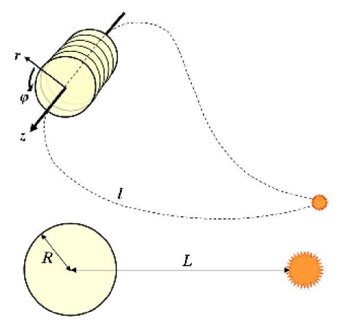
Figure 1: Upper panel: Schematic plot of a flux-rope CME. Lower panel: The cross-section of the flux rope. $R$ is the radius, $L$ is the distance from the flux rope axis to the solar surface, and $l$ is the axial length of the flux rope. The distance, $h$, of the CME leading edge and the minimum and the maximum position angles (indicated by the dot-dashed lines) are the three directly measurable quantities from coronagraph observations.

As commonly assumed, CMEs are approximated as a cylindrical flux rope in a local scale, even though in the global scale they may be a loop-like structure with two ends rooted on the surface of the Sun. The flux rope can therefore be treated axisymmetrically in the cylindrical coordinates ($r$, $\phi$, $z$) with the origin on the axis (ref to Fig.1) and $\frac{\partial}{\partial\phi}=\frac{\partial}{\partial z}=0$. As a result, only a 2-dimensional circular cross-section of the flux rope needs to be considered in our model. Let the radius of the circular cross-section be $R$, the expansion speed of the flux rope is given by

$$v_{e}(t)=\frac{dR(t)}{dt}$$ (1)

Further, assuming that the flux rope is undergoing a self-similar expansion within the cross section, we can get a dimensionless variable

$$x=\frac{r}{R}$$ (2)

which is the normalized radial distance from the flux rope axis and independent of time. The $x=1$ is the boundary of the flux rope. Therefore, the $r$-component of the velocity is

$$v_{r}(t,x)=\frac{dr}{dt}=xv_{e}(t)$$ (3)

and the acceleration is

$$a_{r}(t,x) = \frac{d\mathbf{v}(t,x)}{dt}\cdot\hat{\mathbf{r}}=xa_{e}(t)-\frac{v_{\phi}^{2}(t,x)}{xR}$$ (4)

where

$$a_{e}(t)=\frac{dv_{e}(t)}{dt}$$ (5)

is the acceleration of the expansion. The first term on the right-hand side of Eq.4 is the acceleration of the radial motion of the plasma, and the second term is the acceleration contributed from the circular/poloidal motion.

With the above preliminary preparation, we now investigate an arbitrary fluid element in the flux rope by starting from the momentum conservation equation (in the frame frozen-in with the moving flux rope),

$$\rho\frac{\partial\mathbf{v}}{\partial t}+\rho(\mathbf{v}\cdot\nabla)\mathbf{v}=-\nabla p+\mathbf{j}\times\mathbf{B}$$ (6)

where $\rho$ is the density, $p$ is the plasma thermal pressure, $\mathbf{B}=(0,B_{\phi},B_{z})$ is the magnetic induction, and $\mathbf{j}=\frac{1}{\mu_{0}}\nabla\times\mathbf{B}$ is the current density. Here, the viscous stress tensor, $S$, gravity, $\mathbf{F_{g}}$, and the equivalent force due to the use of a non-inertial reference frame, $\mathbf{F_{a}}$ opposite to the acceleration, are ignored (the validation of this treatment will be discussed at the end of this paper). This equation can be decomposed into the $\hat{r}$ and $\hat{\phi}$ components as follows

$$\hat{r}: \rho\frac{\partial v_{r}}{\partial t}+\rho(v_{r}\frac{\partial v_{r}}{\partial r}-\frac{v_{\phi}^{2}}{r})=-\frac{\partial p}{\partial r}+(\mathbf{j}\times\mathbf{B})_{r}$$ (7)

$$\hat{\phi}: \rho\frac{\partial v_{\phi}}{\partial t}+\rho(v_{r}\frac{\partial v_{\phi}}{\partial r}+\frac{v_{r}v_{\phi}}{r})=0$$ (8)

According to the self-similar assumption, $v_{\phi}$ has the following form

$$v_{\phi}(t,x)=f_{p}(x)v_{p}(t)$$ (9)

in which $f_{p}$ is a function of only $x$ and $v_{p}$ is a function of only $t$. Combine it with Eq.3 and 8, it is inferred that

$$v_{\phi}=k_{1}x^{k_{2}-1}R^{-k_{2}}$$ (10)

where $k_{1}$ and $k_{2}$ are both constants. It is required that $k_{2}\geq 1$ to guarantee that $v_{\phi}$ is physically meaningful, $k_{2}=1$ implies that the angular momentum of the flux rope is conserved, and $k_{2}>1$ means that the angular momentum decreases as the flux rope expands. Combine Eq.2, 3, 7 and 10, we can rewrite the momentum conservation equation with $\hat{r}$ as

$$(\mathbf{j}\times\mathbf{B})_{r}=\rho(a_{e}x-k_{1}^{2}R^{-2k_{2}-1}x^{2k_{2}-3})+R^{-1}\frac{\partial p}{\partial x}$$ (11)

For a thermodynamic process, we relate the thermal pressure $p$ with the density $\rho$ by the polytropic equation of state

$$p=k_{3}\rho^{\Gamma}$$ (12)

where $k_{3}$ is a positive constant and $\Gamma$ is a variable treated as the polytropic index, and Eq.11 becomes

$$(\mathbf{j}\times\mathbf{B})_{r}=\rho(a_{e}x-k_{1}^{2}R^{-2k_{2}-1}x^{2k_{2}-3})+k_{3}R^{-1}\frac{\partial\rho^{\Gamma}}{\partial x}$$ (13)

Define a quantity $f_{em}$ to be the average Lorentz force over $\hat{r}$ from the axis to the boundary of the flux rope, $f_{em}=\frac{1}{R}\int_{0}^{R}(\mathbf{j}\times\mathbf{B})_{r}dr$. From Eq.13, we get

$$f_{em}=a_{e}\int_{0}^{1}\rho xdx-k_{1}^{2}R^{-2k_{2}-1}\int_{0}^{1}\rho x^{2k_{2}-3}dx+k_{3}R^{-1}\int_{0}^{1}\frac{\partial\rho^{\Gamma}}{\partial x}dx$$ (14)

$f_{em}>0$ means that the average Lorentz force directs outward from the axis of the flux rope, causing expansion. On the other hand, $f_{em}<0$ prevents the expansion of the flux rope.

We assume that the mass of a CME is conserved when it propagates in the outer corona and interplanetary space, where the CME has fully developed. The mass conservation gives

$$\int\rho rdrd\phi dz=2\pi lR^{2}\int_{0}^{1}\rho xdx=M\mathrm{\ (constant)}$$ (15)

where $l$ is the axial length of the flux rope (Fig.1). Since the flux rope is assumed to be self-similar and it is generally accepted that the magnetic field lines are frozen-in with the plasma flows in corona/interplanetary space, the density in the flux rope has a fixed distribution $f_{\rho}(x)$, and therefore

$$\rho(t,x)=f_{\rho}(x)\rho_{0}(t)$$ (16)

Define positive constants

$$k_{4}=\int_{0}^{1}f_{\rho}xdx$$ (17)

$$k_{5}=\int_{0}^{1}f_{\rho}x^{2k_{2}-3}dx$$ (18)

and a variable

$$q(\Gamma)=f_{\rho}^{\Gamma}(0)-f_{\rho}^{\Gamma}(1)$$ (19)

Then it can be inferred from Eq.15 that

$$\rho_{0}=\frac{1}{2\pi}k_{4}^{-1}MR^{-2}l^{-1}$$ (20)

and Eq.14 can be written as

$$f_{em}=\frac{M}{2\pi}(a_{e}R^{-2}l^{-1}-k_{1}^{2}k_{4}^{-1}k_{5}R^{-2k_{2}-3}l^{-1})-f_{th}$$ (21)

where

$$f_{th}=\frac{1}{R}\int_{0}^{R}-\frac{\partial p}{\partial r}dr=k_{3}q\rho_{0}^{\Gamma}R^{-1}$$ (22)

is the average thermal pressure force. Like $f_{em}$, $f_{th}$ points outward if it is larger than zero.

On the other hand, in an axisymmetric cylindrical flux rope,

$$\mathbf{B}=B_{\phi}\hat{\phi}+B_{z}\hat{z}=\nabla\times\mathbf{A}$$ (23)

$$B_{\phi}=-\frac{\partial A_{z}}{\partial r}$$ (24)

$$B_{z}=\frac{1}{r}\frac{\partial}{\partial r}(rA_{\phi})$$ (25)

As the magnetic flux is conserved in both $\hat{\phi}$ and $\hat{z}$ directions, we get

$$\Phi_{\phi}=-l\int_{0}^{R}\frac{\partial A_{z}}{\partial r}dr=l(A_{z}(0)-A_{z}(R))$$ (26)

$$\Phi_{z}=2\pi\int_{0}^{R}\frac{\partial}{\partial r}(rA_{\phi})dr=2\pi RA_{\phi}(R)$$ (27)

In order to satisfy the self-similar expansion assumption, $A_{\phi}$ and $A_{z}$ have to keep their own distributions, respectively. Thus, according to the above two equations,

$$A_{\phi}(t,x) = \frac{f_{\phi}(x)}{R}$$ (28)

$$A_{z}(t,x) = \frac{f_{z}(x)}{l}$$ (29)

It can be proved that the conservation of helicity is satisfied automatically

$$H_{m} = \int\mathbf{B}\cdot\mathbf{A}rdrd\phi dz$$ (30)

$$= 2\pi\int_{0}^{1}[\frac{f_{z}}{x}\frac{\partial}{\partial x}(xf_{\phi})-f_{\phi}\frac{\partial f_{z}}{\partial x}]xdx$$

$$= \mathrm{constant}$$

Combining Eq.24, 25, 28 and 29, we can calculate the Lorentz force in the flux rope

$$\mathbf{j}\times\mathbf{B} = \frac{1}{\mu_{0}}(\nabla\times\mathbf{B})\times\mathbf{B}$$ (31)

$$= -\mu_{0}^{-1}R^{-5}\{x^{-2}\frac{\partial}{\partial x}(xf_{\phi})\frac{\partial^{2}}{\partial x^{2}}(xf_{\phi})-x^{-3}[\frac{\partial}{\partial x}(xf_{\phi})]^{2}\}\hat{r}$$

$$-\mu_{0}^{-1}R^{-3}l^{-2}x^{-1}\frac{\partial f_{z}}{\partial x}\frac{\partial}{\partial x}(x\frac{\partial f_{z}}{\partial x})\hat{r}$$

and therefore

$$f_{em} = -\mu_{0}^{-1}R^{-5}\int_{0}^{1}\{x^{-2}\frac{\partial}{\partial x}(xf_{\phi})\frac{\partial^{2}}{\partial x^{2}}(xf_{\phi})-x^{-3}[\frac{\partial}{\partial x}(xf_{\phi})]^{2}\}dx$$ (32)

$$-\mu_{0}^{-1}R^{-3}l^{-2}\int_{0}^{1}x^{-1}\frac{\partial f_{z}}{\partial x}\frac{\partial}{\partial x}(x\frac{\partial f_{z}}{\partial x})dx$$

$$= -\mu_{0}^{-1}k_{6}R^{-5}-\mu_{0}^{-1}k_{7}R^{-3}l^{-2}$$

where $k_{6}$ and $k_{7}$ are both constants. It could be proved that the sign of $k_{6}$ is determined by $B_{z}^{2}(R)-B_{z}^{2}(0)$, and $k_{7}\geq 0$.

The two forms of $f_{em}$, Eq.21 and 32, result in

$$a_{e}-k_{1}^{2}k_{4}^{-1}k_{5}R^{-2k_{2}-1}$$

$$=-2\pi\mu_{0}^{-1}M^{-1}(k_{6}R^{-3}l+k_{7}R^{-1}l^{-1})+2\pi M^{-1}k_{3}(2\pi k_{4}M^{-1}R^{2}l)^{-\Gamma}[f_{\rho}^{\Gamma}(0)-f_{\rho}^{\Gamma}(1)]Rl$$ (33)

in which $f_{th}$ is substituted by Eq.22. As at present it is impossible to practically detect the axial length of a flux rope, here we will relate it with a measurable variable, $L$, the distance between the flux rope axis and the solar surface (Fig.1), at which altitude the flux rope originates, by the assumption

$$l=k_{8}L$$ (34)

where $k_{8}$ is a positive constant. The topology of flux rope as shown in Figure 1 implies that this assumption is reasonable. Finally, Eq.33 can be simplified to

$$a_{e}-c_{0}R^{-c_{1}-3}=-c_{2}R^{-3}L-c_{3}R^{-1}L^{-1}+c_{4}(c_{5}^{\Gamma}-c_{6}^{\Gamma})R^{1-2\Gamma}L^{1-\Gamma}$$ (35)

where

$$c_{0}=k_{1}^{2}k_{4}^{-1}k_{5}\geq 0$$ (36)

$$c_{1}=2k_{2}-2\geq 0$$ (37)

$$c_{2}=2\pi\mu_{0}^{-1}M^{-1}k_{6}k_{8}$$ (38)

$$c_{3}=2\pi\mu_{0}^{-1}M^{-1}k_{7}k_{8}^{-1}\geq 0$$ (39)

$$c_{4}=2\pi M^{-1}k_{3}k_{8}>0$$ (40)

$$c_{5}=(2\pi)^{-1}Mk_{4}^{-1}k_{8}^{-1}f_{\rho}(0)\geq 0$$ (41)

$$c_{6}=(2\pi)^{-1}Mk_{4}^{-1}k_{8}^{-1}f_{\rho}(1)\geq 0$$ (42)

The left-hand side of Eq.35 describes the motion of the fluids in the flux rope. Its first item is the acceleration due to the radial motion (i.e., expansion) and the second one gives the acceleration due to the poloidal motion. The right-hand side reflects the contributions from the Lorentz force (the first two items) and thermal pressure force (the last one). The constants $k_{1-8}$ and $c_{0-6}$ appeared above are summarized in Table 1.

Table 1: List of the constants $k_{1-8}$ and $c_{0-6}$

Constant	Interpretation	Constant	Interpretation
$k_{1}$	Scale the initial magnitude of the poloidal motion	$k_{4}$ and $k_{5}$	Integral constants related to the density distribution
$k_{2}$	Decrease rate of the angular momentum as the flux rope expands	$k_{6}$ and $k_{7}$	Scale the initial magnitude of the Lorentz force contributed by the axial and poloidal fields
$k_{3}$	Coefficient in the polytropic equation of state	$k_{8}$	Assumed constant to relate the length of flux rope $l$ to distance $L$
$c_{0}$	Scale the initial magnitude of the acceleration due to the poloidal motion	$c_{2}$ and $c_{3}$	Similar to $k_{6}$ and $k_{7}$
$c_{1}$	Similar to $k_{2}$	$c_{4}(c_{5}^{\Gamma}-c_{6}^{\Gamma})$	Scale the initial magnitude of the contribution by thermal pressure force

The Lorentz force and thermal pressure force can be rewritten in terms of the constants $c_{0-6}$, $k_{8}$ and the total mass $M$ as follows

$$f_{em}=-\frac{M}{2\pi k_{8}}(c_{2}R^{-5}+c_{3}R^{-3}L^{-2})$$ (43)

$$f_{th}=\frac{M}{2\pi k_{8}}c_{4}(c_{5}^{\Gamma}-c_{6}^{\Gamma})R^{-2\Gamma-1}L^{-\Gamma}$$ (44)

and their ratio is

$$\frac{f_{em}}{f_{th}}=\frac{c_{2}R^{2\Gamma-4}L^{\Gamma}+c_{3}R^{2\Gamma-2}L^{\Gamma-2}}{c_{4}(c_{6}^{\Gamma}-c_{5}^{\Gamma})}$$ (45)

In summary, starting from MHD equations with the three major assumptions that (1) the flux-rope CME has an axisymmetric cylinder configuration, (2) its cross-section is self-similarly evolving, and (3) its axial length is proportional to the distance from the solar surface, we find that the polytropic index, $\Gamma$, can be related to the measurable parameters: the distance, $L$, the radius, $R$, and another derived quantity, the expansion acceleration ($a_{e}$), as shown in Eq.35. If we have enough measurement points, the unknown constants $c_{0-6}$ and variable $\Gamma$ could be obtained through some fitting techniques (e.g., that described in the first paragraph of Sec.3.2), and then the relative strength of the Lorentz force and thermal pressure force can also be easily calculated by Eq.43 and 44.

2.2 Asymptotic Value of Polytropic Index $\Gamma$

Here, we consider the case of a nearly force-free expanding flux rope. It is generally true that most CMEs are almost force-free at least near 1 AU though they may be far away from a froce-free state at initial stage. It can be proved that $R\propto L$ (ref. to Appendix), i.e., $R=\alpha L$ where $\alpha$ is a positive constant. Then Eq.45 becomes

$$\frac{f_{em}}{f_{th}}=\frac{(c_{2}\alpha^{2\Gamma-4}+c_{3}\alpha^{2\Gamma-2})L^{3\Gamma-4}}{c_{4}(c_{6}^{\Gamma}-c_{5}^{\Gamma})}$$ (46)

It is found that $\Gamma=\frac{4}{3}$ is a critical point, above/below which the absolute value of Lorentz force decreases slower/faster than that of thermal pressure force as increasing distance $L$. This value of $\Gamma$ is the same as that obtained by Low [1982] and Kumar and Rust [1996] for a self-similar expanding flux rope. This inference is reasonable because smaller $\Gamma$ implies the plasma absorbs more heat for the same expansion and therefore the thermal pressure should decrease slower.

Under force-free condition, Eq.35 can also reduce to

$$a_{e}=c_{0}(\alpha L)^{-c_{1}-3}-c_{2}\alpha^{-3}L^{-2}-c_{3}\alpha^{-1}L^{-2}+c_{4}(c_{5}^{\Gamma}-c_{6}^{\Gamma})\alpha^{1-2\Gamma}L^{2-3\Gamma}$$ (47)

and at infinite distance, $L\rightarrow+\infty$, we have

$$a_{e\infty}\sim c_{4}(c_{5}^{\Gamma_{\infty}}-c_{6}^{\Gamma_{\infty}})\alpha^{1-2{\Gamma_{\infty}}}L_{\infty}^{2-3{\Gamma_{\infty}}}$$ (48)

The above equation indicates that $\Gamma=\frac{2}{3}$ is another critical point. The polytropic index $\Gamma$ should be larger than $\frac{2}{3}$ to make sure that the flux rope will finally approach a steady expansion and propagation state (including the case that the flux rope stop somewhere without expansion). Otherwise, the flux rope will always accelerated expanding.

Based on the current observations, the expansion behavior of CMEs at large heliocentric distance is not as clear as that in the inner heliosphere. The investigations on the radial widths of CMEs suggest that CMEs at least keep expanding within about 15 AU [e.g., Wang and Richardson, 2004; Wang et al., 2005], but the expansion speeds seem to be slower and slower. Although the number of CMEs observed near and beyond 15 AU is small and the uncertainty of statistics is large, it is likely that a CME may not be able to keep an accelerated expansion always. Thus, in practice, the polytropic index of the CME plasma should be larger than $\frac{2}{3}$.

3 The 2007 October 8 CME

3.1 Observations and Measurements

The suite of SECCHI instruments on board STEREO spacecraft provide an unprecedented continuous view of CMEs from the surface of the Sun through the inner heliosphere. The instruments, EUVI, COR1, COR2, HI1 and HI2, make the images of the solar corona in the ranges of 0–1.5, 1.4–4.0, 2.5–15.0, $\sim$15–90, and $\sim$90–300 solar radii ($R_{S}$), respectively [Howard et al., 2008]. The SECCHI observations present us the great opportunity to study the evolution of CMEs over an extended distance. The CME launched on 2007 October 8 is a well observed event, which is used to study the CME evolution and the applicability of our model.

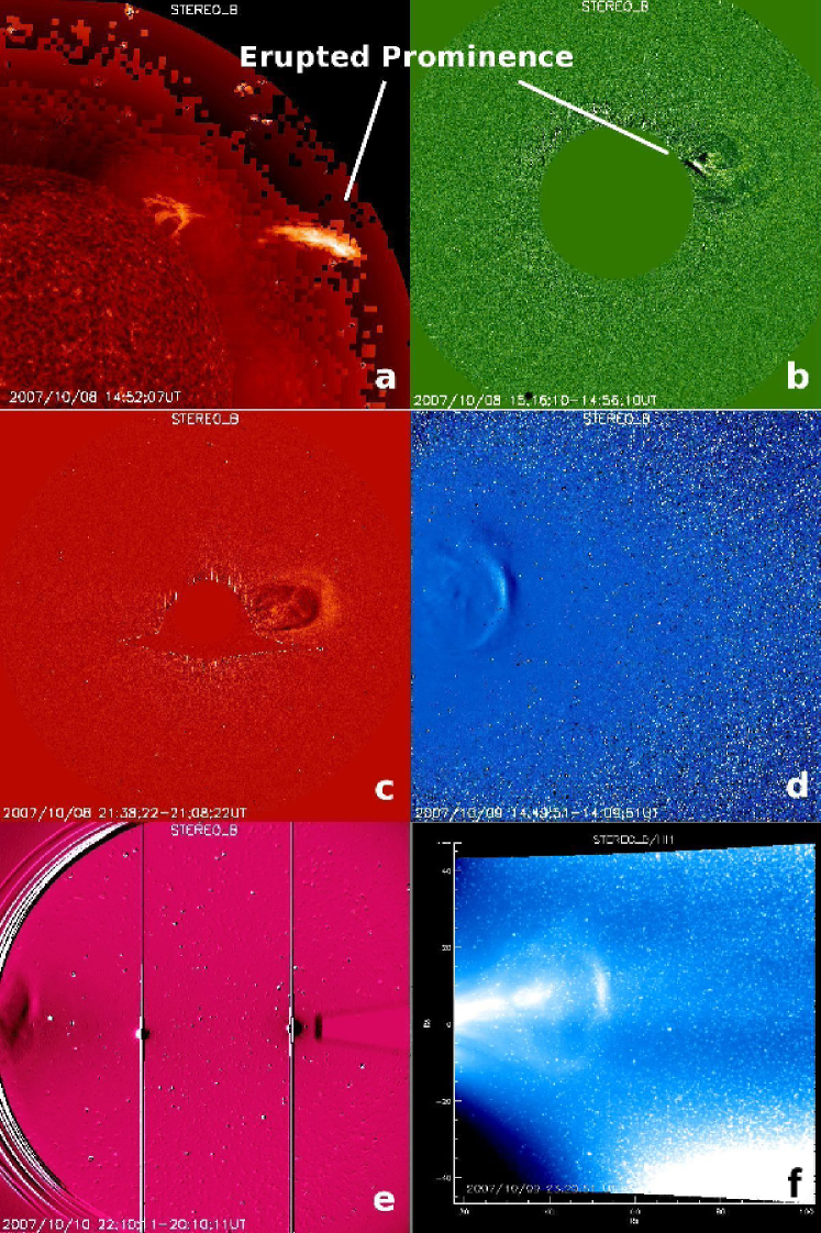
Figure 2: Images of the 2007 October 8 CME taken by (a) EUVI at 304Å, (b) COR1, (c) COR2, (d) HI1 and (e) HI2 on board STEREO B. The panel at lower-right corner shows a direct image of the CME in the HI1 FOV. This image has been corrected to the plane perpendicular to the line between the Sun and STEREO B, because the CME is assumed to be a limb event in CORs and the direction that HI1 camera faces to is different with CORs’.

This CME was initiated close to the western limb as seen from STEREO B. Hereafter all the observations used are from instruments on board the B spacecraft. Figure 2 shows five images of the CME at different distances from the Sun. The CME was accompanied by a prominence eruption starting at about 07:00 UT on October 8, as seen by EUVI. The CME source region is clearly shown in the EUVI 304Å image on the top-left panel of the figure. The erupting prominence was also seen in the COR1 running-difference image (the top-right panel). The CME was first observed in COR1 at about 08:46 UT on October 8, and continuously ran through COR2 and HI1 fields of view (FOV). It even showed in the HI2 FOV after about 12:00 UT on October 10. Since the CME was launched from the western limb and showed a circular-like structure, we believe that the CME was viewed by the instruments through an axial-view angle. Therefore, the projection of the CME on the plane of the sky can be treated as the cross-section of the CME.

To obtain the two quantities, $R$ and $L$, for necessary model inputs, here we simply measure three parameters, the heliocentric distance of the CME leading edge, $h$, and the maximum and minimum position angles, $\theta_{max}$ and $\theta_{min}$, of the CME as shown in Figure 1. Under the assumption of a circular cross-section, $R$ and $L$ could be derived by

$$R = h-L-R_{S}$$ (49)

$$L = \frac{h}{1+\sin\frac{\theta_{max}-\theta_{min}}{2}}-R_{S}$$ (50)

It should be noted that the measurements in HI2 images are not included in the following analysis, because the elongation effect is not negligible.

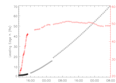
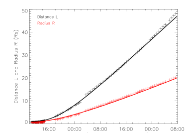
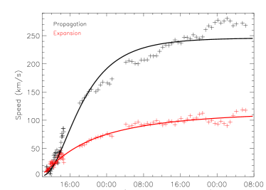
Figure 3: Left-upper panel: The measurements of the heliocentric distance, $h$, of the flux-rope CME leading edge and its angular width, $\Delta\theta=\theta_{max}-\theta_{min}$. Right panel: The derived distance, $L$, of the flux rope axis from the solar surface and the flux rope radius, $R$. Left-lower panel: The propagation, $v_{c}$, and expansion, $v_{e}$, speeds derived from $L$ and $R$, respectively.

Figure 3 shows the measurements and the derived parameters. The CME is a slow and gradually accelerated event. It took about 46 hours for its leading edge to reach 70 $R_{S}$. Nevertheless, because of its slowness, we are able to make about one hundred measurement points for this CME. The red crosses plotted in the leftupper panel suggests that the CME angular width increased at the early phase (mainly in the COR1 FOV), and then reached to a near-constant value in the COR2 and HI1 FOVs. The right panel presents the evolution of the derived $R$ and $L$. It is shown that the radius of the flux-rope CME is about 20 $R_{S}$ when it propagated nearly 50 $R_{S}$ away from the Sun, which put the leading edge at about 70 $R_{S}$. The left-lower panel exhibits the speeds derived from the $R$ and $L$, namely expansion, $v_{e}$ and propagation, $v_{c}$, speeds, respectively. At the early phase, the expansion speed was very close to the propagation speed. In the later phase, the propagation speed increased more quickly than the expansion speed. The increased difference between $v_{c}$ and $v_{e}$ is probably because of (1) the enhanced drag force of the ambient solar wind, which is fully formed in the outer corona and (2) the weakened pressure in the CME. The issue of CME acceleration, which is as important as CME expansion, is not addressed in our model presented in this paper.

In the measurements, the CME radius obtained is the one along the latitudinal direction on the meridional plane. This radius would be the same as the radius along the radial direction if the cross-section is a perfect circle. However, the true cross-section deviates from the perfect circle, and the deviation becomes larger as the CME is further from the Sun [e.g., Riley and Crooker, 2004]. The distortional stretching of the cross-section is caused by the divergent radial expansion of the background solar wind, which causes kinematic expansion of CMEs along both the meridional and azimuthal directions, but not at all along the radial direction. The CME expansion along the radial direction is mostly driven by the dynamic effect, such as pressure gradient forces, while the expansion along the other two directions that lie on the spherical surface is caused by the combination of the dynamic and kinematic effects. As a result, the overall cross-section is a convex-outward “pancake” shape [Riley and Crooker, 2004]. Figure 2f shows such a distortion of the 2008 November 8 CME as observed in HI1 FOV; the aspect ratio, defined by the ratio of the radius along the meridional direction and that along the radial direction, is about 1.4 when the CME leading edge is at $\sim 70R_{S}$.

Due to this stretching effect, our measurements assuming a circular cross-section lead to the inaccuracy of the measured parameters and the inferred parameters as well. In order to study the internal state of a CME, the radius of the CME, $R$, should be the one along the radial direction, and it is apparently overestimated when the radius along the meridional direction is adopted. The derived expansion speed of CME is thus larger than the true value. Such simplified measurements would infer unrealistic parameters of CME at 1 AU. For instance, the observed radius of 20 $R_{S}$ of the CME at a distance of 50 $R_{S}$ from the Sun would imply a CME cross-section of 0.8 AU at 1 AU, which is too larger to be true. The observed speeds of $v_{e}$ and $v_{c}$ would imply a speed of about 150 km/s at the trailing edge of the CME, which is much smaller than the observed solar wind speed, i.e., about 300 km/s. Therefore, one should be cautious when our method is applied to CMEs at a large distance from the Sun (e.g, $>70R_{S}$). The heliospheric region we investigated in this paper is within about 70 $R_{S}$, and the stretching effect is relatively small. Nevertheless, we will carefully estimate the errors on CME parameters in the second paragraph of Sec.5. We point out here that there is an observational difficulty in measuring the radius of CMEs along the radial direction in a consistent way, mainly because of the low brightness contrast of the CME trailing edge in coronagraph images. This difficulty might be overcome if the CME of interest is particularly bright.

Before modeling the CME, we fit the measurement points with a certain function to retrieve the smooth evolution process of the CME, which is required for the model. We use the modified function of log normal distribution to fit the speeds. We did not fit the expansion acceleration directly, because any small error in measurements of $R$ will be dramatically amplified in its second derivative $a_{e}$. The fitting function of velocity has the form

$$v(t)=\frac{v_{\infty}}{2}\left[1+\mathrm{erf}\left(\frac{\ln(t-t_{0})-M}{S\sqrt{2}}\right)\right]$$ (51)

where $\mathrm{erf}(z)$ is the erf function or error function, defined by

$$\mathrm{erf}(z)\equiv\frac{2}{\sqrt{\pi}}\int_{0}^{z}e^{-t^{2}}dt$$ (52)

This function has a value range from 0 to $v_{\infty}$. It is chosen because the measurements show a trend that, at least within the FOVs of SECCHI, both the speeds will not increase forever, but instead asymptotically approach a constant speed, $v_{\infty}$. The acceleration can be derived by

$$a_{e}(t)=\frac{v_{\infty}}{S\sqrt{2\pi}(t-t_{0})}e^{-\frac{[\ln(t-t_{0})-M]^{2}}{2S^{2}}}$$ (53)

The solid lines in the left-lower panel of Figure 3 show the fitting results. The fitted parameter $v_{\infty}$ is 118 km/s for expansion and 246 km/s for propagation. As a comparison with the measurements, the integrals of the fitting curves of the speeds are also plotted in the right panel. It has been mentioned before that these estimated speeds suffer the solar wind stretching effect. Particularly, the estimated expansion speed is larger than that it should be. The error will be discussed in Sec.5.

3.2 Results

To fit the above curves with the model, Eq.35, we use an iterative method. Generally speaking, first we solve this equation in every 8 neighboring measurement points to obtain a set of parameters $c_{0-6}$ and $\Gamma$. The segment of the 8 points is a running box through the entire evolution process of the CME. Secondly, input the obtained variable $\Gamma$ into the model as guess values to fit the global constants $c_{0-6}$. Thirdly, use the fitted $c_{0-6}$ to update the variable $\Gamma$ by solving Eq.35 again. Then iterate the above 2nd and 3rd steps to make constants $c_{0-6}$ and $\Gamma$ converging to a steady solution. For the sake of simplicity, we ignore the poloidal motion of the fluid by setting $c_{0}$ zero. It is also because there seems no strong observational evidence showing a ring flow inside a CME.

The model results are shown in Figure 4. The uncertainty of the model results is estimated from the relative error of $a_{e}$, which is given by

$$E=\left|\frac{a_{em}-a_{ei}}{a_{ei}}\right|$$ (54)

where $a_{ei}$ is the value calculated by the input data, and $a_{em}$ is the model value. The error curve is plotted in the left-upper panel of Figure 4. It is found that the error is smaller than 1%, except during 12:00 – 18:00 UT. A possible explanation of the large uncertainty during that time has been given in the last second paragraph of Sec.5.

3.2.1 Polytropic Index

From the right-upper panel of Figure 4, it is found that $\Gamma$ was less than 1.4 throughout the interplanetary space. In the inner corona, say $L\;\lower 4.0pt\hbox{${\buildrel\displaystyle<\over{\sim}}$}\;2R_{S}$, it was about 1.24. After entering the outer corona, it quickly increased to above 1.35 at $L\approx 5R_{S}$, and then slowly approached down to about 1.336, which is very close to the first critical point $\frac{4}{3}$. This value of $\Gamma$ is consistent with the observational value obtained from Liu et al. [2006] statistics for protons. As the CME kept expanding during its propagation in the FOVs, the polytropic index less than $\frac{5}{3}$ means that there must be some mechanisms to inject heat from somewhere into the CME plasma. Although the CME plasma continuously got thermal energy, the proton temperature may be still much lower than that in the ambient solar wind, as revealed by many in-situ observations of MCs [e.g., Burlaga et al., 1981].

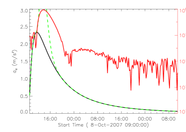
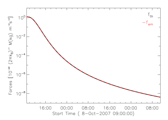
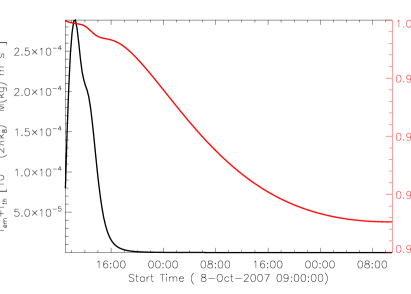
Figure 4: Left-upper panel: The profile of $a_{e}$ (black), the modeled result (dashed green), and the relative error (see text for details). Right-upper panel: The variation of the polytropic index, $\Gamma$, of the CME plasma. Left-lower panel: The variations of the average Lorentz force, $f_{em}$, and the average thermal pressure force, $f_{th}$. Their signs have been marked on the upper right corner. Right-lower panel: The sum and ratio of the two forces.

We believe that the hot plasmas in the lower solar atmosphere is probably a major heat source of CMEs in the interplanetary space. As shown in Figure 1, a CME is believed to be a looped structure with two ends rooted on the solar surface in a global scale. Bidirectional electron streams are one of the evidence of it [e.g. Farrugia et al., 1993; Larson et al., 1997]. Thus it is possible that heat is conducted from the bottom to CMEs. The ambient solar wind with higher temperature might be an additional source because the temperature difference between the two mediums is significant. However, the cross-field diffusion of particles are much more difficult than the motion parallel to magnetic field lines, especially in a nearly force-free flux rope; the coefficient ratio $\kappa_{\perp}/\kappa_{\parallel}$ of perpendicular to parallel diffusion roughly locates in the range of $0.005-0.05$ [e.g., Jokipii et al., 1995; Giacalone and Jokipii, 1999; Zank et al., 2004; Bieber et al., 2004]. Thus the contribution of the ambient high-temperature solar wind should be very limited.

It is well known that the magnetic energy decreases as CMEs propagate away from the Sun. According to our model, the total magnetic energy is given by

$$E_{m}=\frac{1}{2\mu_{0}}\int B^{2}rdrd\phi dz=\pi\mu_{0}^{-1}(k_{9}l^{-1}+k_{10}R^{-2}l)$$ (55)

where

$$k_{9}=\int_{0}^{1}(\frac{\partial f_{z}}{\partial x})^{2}xdx$$ (56)

$$k_{10}=\int_{0}^{1}[\frac{\partial}{x\partial x}(xf_{\phi})]^{2}xdx$$ (57)

are both positive integral constants. The magnetic energy generally dissipates at the rate of $\sim l^{-1}$, which is a significant dissipation as CMEs move outward. However, such magnetic energy dissipation does not necessarily mean to be a major source of the heat. According to MHD theory, magnetic energy partially goes into kinetic energy and partially converts to thermal energy. The former is due to the work done by Lorentz force ($\mathbf{j}\times\mathbf{B}\cdot\mathbf{u}$), and the latter is through the Joule heating ($\frac{j^{2}}{\sigma}$) process, where $j$ is the current density and $\sigma$ is the electrical conductivity. Since $\sigma$ usually has a large value in interplanetary medium, without anomalous resistivity, the magnetic energy does not have an efficient way to be converted to thermal energy. However, there are possibly many non-ideal processes, such as turbulence, but not accounted by MHD theory. Thus we do not know whether the dissipated magnetic energy is a major source of heating or not.

3.2.2 Internal Forces

The averaged Lorentz force, $f_{em}$, and thermal pressure force, $f_{th}$, have been presented in the left-lower panel of Figure 4. Their absolute values are very close to each other, and both of them decreased continuously throughout the interplanetary space. The signs of the two forces are opposite. $f_{em}$ is negative indicating a centripetal force, whereas $f_{th}$ is positive, centrifugal. This result suggests that the thermal pressure force contributed to the CME expansion, but the Lorentz force prevented the CME from expanding.

The difference between the two forces can be seen more clear from the right-lower panel of Figure 4. The black line exhibits the net force, $f_{em}+f_{th}$, inside the CME. It directed outward and reached the maximum at about 10:30 UT. The profile is consistent with the expansion acceleration presented in the left-upper panel (the black line). Thus the net force just shows us the internal cause of the CME expansion. The red line is the ratio of their absolute values. Its value changed in a very small range from about 1.0 to 0.98. It suggests that such a small difference between the two forces is able to drive the CME expanding with the acceleration at the order of 1 $m/s^{2}$. Moreover, the ratio decrease means that the Lorentz force decreased slightly faster than the thermal pressure force. One may notice that, since $\Gamma$ was larger than the first critical point $\frac{4}{3}$ at $L\;\lower 4.0pt\hbox{${\buildrel\displaystyle>\over{\sim}}$}\;5R_{S}$, according to the analysis in Sec.2.2, the Lorentz force should drop slower than thermal pressure force. Actually it may not be an inconsistency, because the inference derived in Sec.2.2 is established on the force-free assumption, the CME we studied may not be perfectly force-free, and therefore the first critical point of $\Gamma$ probably shifts a little bit.

Usually, CMEs are a flux rope with two ends rooted on the Sun. The axial curvature of the flux rope may cause the magnetic strength at the Sun-side of the flux rope larger than that at the opposite side, which leads the Lorentz force having an additional component to drive the flux rope moving outward away from the Sun [e.g., Garren and James, 1994; Lin et al., 1998, 2002; Kliem and Török, 2006; Fan and Gibson, 2007]. Thus, as the flux rope we applied here is assumed to be a straight cylinder, the Lorentz force $f_{em}$ we derived does not include the component caused by the axial curvature of the flux rope. This component is important in studying the propagation properties of a CME. However, our model is to study the CME internal state (specifically the thermodynamic process and expansion behavior), and its propagation behavior is obtained directly from coronagraph observations, thus the neglect of this component should be acceptable although it does bring on some error, which has been briefly mentioned in the second paragraph of Sec.5.

4 Summary

In this paper, we developed an analytical flux rope model for the purpose of probing the internal state of CMEs and understanding its expansion behavior. The model suggests that, if the flux rope is force free, there are two critical values for the polytropic index $\Gamma$. One is $\frac{4}{3}$, above/below which the absolute value of the Lorentz force decreases slower/faster than that of the thermal pressure force as the flux-rope CME propagates away from the Sun. The other is $\frac{2}{3}$, above which the flux-rope CME will essentially approach a steady expansion and propagation state.

By applying this model to the 2007 October 8 CME event, we find that (1) the polytropic index of the CME plasma increased from initially 1.24 to more than 1.35 quickly, and then slowly decreased to about 1.336; it suggests that there be continuously heat injected/converted into the CME plasma and the value of $\Gamma$ tends to be the first critical value $\frac{4}{3}$; (2) the Lorentz force directed inward while the thermal pressure force outward, both of them decreased rapidly as the CME moved out, and the small difference between them is consistent with the expansion acceleration of the CME; the direction of the two forces reveal that the thermal pressure force is the internal driver of the CME expansion, whereas the Lorentz force prevented the CME from expanding.

5 Discussion

In our model, the interaction between CMEs and the solar wind has been implicitly included to certain extent, though we do not explicitly address these effects. The consequences of the interaction, in terms of the effects on the CME dynamic evolution can be roughly classified into the following three types: (1) the solar wind dragging effect, which is is due to the momentum exchange between the CME plasma and the ambient solar wind and mainly affects the CME’s propagation speed or the bulk motion speed, (2) the solar wind constraint effect on expansion, which is caused by the presence of the external magnetic and thermal pressures and mainly prevents a free expansion of the CME (i.e., in all directions), and (3) the solar wind stretching effect on expansion, which is caused by the divergent radial expansion of solar wind flow, and causes flattening or “pancaking” of CMEs. The first two effects are indirectly included in the model through the measurements of $L$ and $R$. Different dragging and/or constraint force(s) may result in different variation of $L$ and/or $R$ with time (or heliocentric distance). Particularly, we do not need to explicitly put the solar wind dragging term in the model, because we are addressing the internal state of CMEs, not the bulk acceleration. The stretching effect, which is of a kinematic effect, is not included in our model. As discussed in the sixth paragraph of Sec.3.1, this is largely due to the limitation of the measurements. The possible errors caused by such effect are explicitly addressed in the next paragraph.

The main uncertainty of this model, we believe, comes from the assumption of an axisymmetric cylinder, in which the curvature of the axis of the flux rope and the distortion of the circular cross-section are not taken into account. As to the first one, the neglect of the axial curvature generally results in the Lorentz force underestimated. As to the second one, as discussed earlier, the distortion of the CME cross-section is due to the kinematic stretching effect of a spherically divergent solar wind flow [e.g., Crooker and Intriligator, 1996; Russell and Mulligan, 2002; Riley et al., 2003; Riley and Crooker, 2004; Liu et al., 2006]. In the case of the particular CME studied in this paper, the aspect ratio is about 1.4 when the CME leading edge is at $\sim 70R_{S}$ (or the flux rope axis is at $\sim 56R_{S}$). The overall shape of the CME looks like an ellipse. To estimate the errors caused by the circular assumption, we approximate the ellipse to be a circle of the same area. With this treatment, we estimate that $R$ is overestimated by 19%, and $L$ is underestimated by 11%. Therefore, the expansion speed is overestimated by 19%, and the propagation speed is underestimated by 11%. Further, we find that the density is underestimated by 21% (ref to Eq.20), $f_{th}$ is underestimated by 39% (ref to Eq.22 and assume $\Gamma=\frac{4}{3}$), $f_{em}$ is underestimated by 25–58% (ref to Eq.32), and the error of the polytropic index is probably neglected (ref. to Eq.44). These errors are evaluated for the CME at $\sim 70R_{S}$. At a smaller distance, we expect that the errors be smaller, since the distortion is less severe.

The self-similar assumption made in our model may be another error source, in which we assume that the distributions of the quantities along $\hat{\mathbf{r}}$ in the flux rope remain unchanged during the CME propagates away from the Sun. Self-similar evolution is a frequently used assumption in modeling [e.g., Low, 1982; Kumar and Rust, 1996; Gibson and Low, 1998; Krall and St. Cyr, 2006]. The recent research by Démoulin and Dasso [2009] suggested that, when $l$, the length of flux rope, is proportional to $p_{t}^{-1/4}$, the total pressure in the ambient solar wind, a force-free flux rope will evolve self-similarly. The total pressure of solar wind consists of thermal pressure $p_{th}=nkT$ and magnetic pressure $p_{m}=\frac{B^{2}}{2\mu}$. Near the Sun, we can assume that the magnetic pressure is dominant, thus it is approximated that $p_{t}\approx p_{m}\propto L^{-4}$, i.e., $p_{t}^{-1/4}\propto L$. Since the length of a flux rope is usually proportional to the distance $L$, we have $l\propto p_{t}^{-1/4}$. It means that self-similar assumption should be a good approximation when the CME is nearly force-free and not too far away from the Sun. Other previous studies also showed that the self-similar evolution of CMEs is probably true within tens solar radii [e.g., Chen et al., 1997; Krall et al., 2001; Maričić et al., 2004]. On the other hand, however, the self-similar assumption must be broken gradually. An obvious evidence is from the solar wind stretching effect as have been addressed before. Another evidence is that a CME may relax from a complex structure to a nearly force-free flux rope structure, for example the simulation by Lynch et al. [2004].

For the CME plasma, neglecting the viscous stress tensor in Eq.6 might be appropriate. The viscous stress tensor of protons can be approximately given by

$$S_{ij}\approx 3\eta_{0}\left(\frac{\delta_{ij}}{3}-\frac{B_{i}B_{j}}{B^{2}}\right)\left(\frac{\mathbf{B}\cdot\mathbf{B}\cdot\nabla\mathbf{v}}{B^{2}}-\frac{\nabla\cdot\mathbf{v}}{3}\right)$$ (58)

and $\eta_{0}$ is the coefficient of viscosity that could be estimated by $\eta_{0}\approx 10^{-17}T_{p}^{\frac{5}{2}}$ kg$\cdot$m${}^{-1}\cdot$s^-1 [Braginskii, 1965; Hollweg, 1985]. Here $\delta_{ij}$ is the unit tensor, $\mathbf{v}$ is flow velocity, and $T_{p}$ is the proton temperature. Since the proton temperature in CMEs is low, $\eta_{0}$ and therefore the viscous stress tensor is very small. Thus, we guess that the viscosity in the momentum equation might be ignored.

Both forces ignored in Eq.6, the gravity $\mathbf{F}_{g}$ and the equivalent fictitious force $\mathbf{F}_{a}$ due to the use of a non-inertial reference frame, are in the radial direction in the solar frame. Their effects can be evaluated by comparing them with the acceleration of the expansion of the fluids in flux rope CMEs. The solar gravity acceleration is about 270 m/s² at the surface, and decreases at the rate of $r^{-2}$, which makes it as low as $\sim$2.7 m/s² at 10 $R_{S}$. And $\mathbf{F}_{a}$ should be also very small for most CMEs beyond 10 $R_{S}$. Thus both forces would significantly distort the model results only on CMEs with slow expansion acceleration in the lower corona, but not on those with large expansion acceleration or in the outer corona. This may be the reason why a large error of $a_{e}$ appears during 12:00 – 18:00 UT in modeling this CME (left-upper panel of Fig.4).

The flux-rope model presented in this paper might be the first of its kind to provide a way to infer the inter state of CMEs directly based on coronagraph observations. It is different from other CME dynamic models, such as those by Chen [1989] and Gibson and Low [1998], which were designed to study the interaction of CMEs with the ambient solar wind and other dynamic processes by adjusting the initial conditions of CMEs and the global parameters of the ambient solar wind. Besides, Kumar and Rust [1996] proposed a current-core flux rope model with self-similar evolution (ref. to KR model thereafter). Although a self-similar flux rope is also employed in their model, our model is largely different from theirs. First, the flux rope in KR model is assumed force-free and the Lundquist solution [Lundquist, 1950] is applied to describe the internal magnetic structure, but our model does not specify the magnetic field distribution and it may be non-force-free. Secondly, the self-similar assumption in KR model limits the radius of the flux rope to be proportional to the distance, whereas our self-similar condition is held only in the cross-section of the flux rope; the $R$ and $L$ in our model are two independent measurements (see Fig.3). Thirdly, KR model did not consider the solar wind effects on the flux rope, while two of three solar wind effects are implicitly included in our model. Thus one can treat our model a more generic one. Undoubtedly, KR model is an excellent model for force-free flux ropes, and got many interesting results. For example, it is suggested that the polytropic index is $\frac{4}{3}$ for a CME far from the Sun. It is an inference from their self-similar assumption, and it seems to be true for the 2007 October CME we studied here. In our model, the $\Gamma$ value of $\frac{4}{3}$ implies a special case (Sec.2.2) in which the two internal forces $f_{em}$ and $f_{th}$ vary at the same rate. Further work will be performed to test whether it holds for all CME events.

Acknowledgments.

We acknowledge the use of the data from STEREO/SECCHI. We are grateful to James Chen and Yong C.-M. Liu for discussions. We also thank the referees for valuable comments. Y. Wang and J. Zhang are supported by grants from NASA NNG05GG19G, NNG07AO72G, and NSF ATM-0748003. Y. Wang and C. Shen also acknowledge the support of China grants from NSF 40525014, 973 key project 2006CB806304, and Ministry of Education 200530.

Appendix

In cylindrical coordinate system, the magnetic field of a force-free flux rope has the Lundquist [1950] solution

$$B_{r} = 0$$

$$B_{\phi} = HB_{0}J_{1}(2.41x)$$ (59)

$$B_{z} = B_{0}J_{0}(2.41x)$$

where $x=\frac{r}{R}$ is the normalized radial distance as defined in Sec.2, $J_{0}$ and $J_{1}$ are the zero and first order Bessel functions, $H=\pm 1$ indicates the sign of the handedness and $B_{0}$ is the magnetic field magnitude at the axis of the flux rope. According to the properties of Bessel function, we have the magnetic vector potential

$$A_{\phi} = \frac{RB_{0}}{2.41}J_{1}(2.41x)$$ (60)

$$A_{z} = \frac{HRB_{0}}{2.41}J_{0}(2.41x)$$ (61)

The conservation of $\Phi_{z}$

$$\Phi_{z}=2\pi\int_{0}^{R}\frac{\partial}{\partial r}(rA_{\phi})dr=\frac{2\pi R^{2}B_{0}}{2.41}J_{1}(2.41)=\mathrm{constant}$$ (62)

requires that

$$B_{0}=2.41a_{1}R^{-2}$$ (63)

where $a_{1}$ is a constant. The magnetic vector potential can be rewritten as

$$A_{\phi} = \frac{a_{1}}{R}J_{1}(2.41x)$$ (64)

$$A_{z} = \frac{a_{1}H}{R}J_{0}(2.41x)$$ (65)

Meanwhile, the magnetic helicity is

$$H_{m}=\int\mathbf{B}\cdot\mathbf{A}drrd\phi dz=4.82\pi a_{1}^{2}a_{2}HR^{-1}l$$ (66)

where $a_{2}=\int_{0}^{1}x(J_{0}^{2}+J_{1}^{2})dx$ is a constant. The conservation of $H_{m}$ results in

$$R\propto l$$ (67)

Combined it with the assumption Eq.34, it is inferred that

$$R\propto L$$ (68)

which means that the force-free flux rope expands radially.

References

- Akmal et al. [2001] Akmal, A., J. C. Raymond, A. Vourlidas, B. Thompson, A. Ciaravella, Y.-K. Ko, M. Uzzo, and R. Wu (2001), SOHO observations of a coronal mass ejection, Astrophys. J., 553, 922–934.
- Antonucci et al. [1997] Antonucci, E., J. L. Kohl, G. Noci, G. Tondello, M. C. E. Huber, L. D. Gardner, P. Nicolosi, S. Giordano, D. Spadaro, A. Ciaravella, C. J. Raymond, G. Naletto, S. Fineschi, M. Romoli, O. H. W. Siegmund, C. Benna, J. Michels, A. Modigliani, A. Panasyuk, C. Pernechele, P. L. Smith, L. Strachan, , and R. Ventura (1997), Velocity fields in the solar corona during mass ejections as observed with UVCS-SOHO, Astrophys. J., 490, L183–L186.
- Bieber et al. [2004] Bieber, J. W., W. H. Matthaeus, A. Shalchi, and G. Qin (2004), Nonlinear guiding center theory of perpendicular diffusion: General properties and comparison with observation, Geophys. Res. Lett., 31, L10,805.
- Braginskii [1965] Braginskii, S. I. (1965), Transport processes in a plasma, Rev. Plasma Phys., 1, 205.
- Burlaga et al. [1981] Burlaga, L., E. Sittler, F. Mariani, and R. Schwenn (1981), Magnetic loop behind an interplanetary shock: Voyager, Helios, and IMP 8 observations, J. Geophys. Res., 86(A8), 6673–6684.
- Chen [1989] Chen, J. (1989), Effects of toroidal forces in current loops embedded in a background plasma, Astrophys. J., 338, 453–470.
- Chen et al. [1997] Chen, J., R. A. Howard, G. E. Brueckner, R. Santoro, J. Krall, S. E. Paswaters, O. C. St. Cyr, R. Schwenn, P. Lamy, and G. M. Simnett (1997), Evidence of an erupting magnetic flux rope: Lasco coronal mass ejection of 1997 april 13, Astrophys. J., 490, L191.
- Ciaravella et al. [2000] Ciaravella, A., J. C. Raymond, B. J. Thompson, A. Van Ballegooijen, L. Strachan, J. Li, L. Gardner, R. O’Neal, E. Antonucci, J. Kohl, and G. Noci (2000), Solar and heliospheric observatory observations of a helical coronal mass ejection, Astrophys. J., 529, 575–591.
- Ciaravella et al. [2001] Ciaravella, A., J. C. Raymond, F. Reale, L. Strachan, and G. Peres (2001), 1997 December 12 helical coronal mass ejection. II. density, energy estimates, and hydrodynamics, Astrophys. J., 557, 351–365.
- Ciaravella et al. [2003] Ciaravella, A., J. C. Raymond, A. Van Ballegooijen, L. Strachan, A. Vourlidas, J. Li, J. Chen, and A. Panasyuk (2003), Physical parameters of the 2000 February 11 coronal mass ejection: Ultraviolet spectra versus white-light images, Astrophys. J., 597, 1118–1134.
- Crooker and Intriligator [1996] Crooker, N. V., and D. S. Intriligator (1996), A magnetic cloud as a distended flux rope occlusion in the heliospheric current sheet, J. Geophys. Res., 101(A11), 24,343–24,348.
- Démoulin and Dasso [2009] Démoulin, P., and S. Dasso (2009), Causes and consequences of magnetic cloud expansion, Astron. & Astrophys., 498, 551–566.
- Fan and Gibson [2007] Fan, Y., and S. E. Gibson (2007), Onset of coronal mass ejections due to loss of confinement of coronal flux ropes, Astrophys. J., 668, 1232–1245.
- Farrugia et al. [1993] Farrugia, C. J., I. G. Richardson, L. F. Burlaga, R. P. Lepping, and V. A. Osherovich (1993), Simultaneous observations of solar mev particles in a magnetic cloud and in the earth’s northern tail lobe: Implications for the global field lines topology of magnetic clouds and entry of solar particles into the tail lobe during cloud passage, J. Geophys. Res., 98, 15,497.
- Forbes and Isenberg [1991] Forbes, T. G., and P. A. Isenberg (1991), A catastrophe mechanism for coronal mass ejections, Astrophys. J., 373, 294–307.
- Garren and James [1994] Garren, D. A., and C. James (1994), Lorentz self-forces on curved current loops, Phys. Plasma, 1, 3425–3436.
- Giacalone and Jokipii [1999] Giacalone, J., and J. R. Jokipii (1999), The transport of cosmic rays across a turbulent magnetic field, Astrophys. J., 520, 204.
- Gibson and Low [1998] Gibson, S. E., and B. C. Low (1998), A time-dependent three-dimensional magnetohydrodynamic model of the coronal mass ejection, Astrophys. J., 493, 460.
- Goldstein [1983] Goldstein, H. (1983), On the field configuration in magnetic clouds, in Sol. Wind Five, p. 731, NASA Conf. Publ. 2280, Washington D. C.
- Hollweg [1985] Hollweg, J. V. (1985), Viscosity in a magnetized plasma: Physical interpretation, J. Geophys. Res., 90(A8), 7620–7622.
- Howard et al. [2008] Howard, R. A., J. Moses, A. Vourlidas, and et al. (2008), Sun earth connection coronal and heliospheric investigation (SECCHI), Space Sci. Rev., 136, 67–115.
- Jian et al. [2008] Jian, L., C. Russell, J. Luhmann, R. Skoug, and J. Steinberg (2008), Stream interactions and interplanetary coronal mass ejections at 5.3 AU near the solar ecliptic plane, Sol. Phys., 250, 375–402.
- Jokipii et al. [1995] Jokipii, J. R., J. Kota, J. Giacalone, T. S. Horbury, and E. J. Smith (1995), Interpretation and comsequenes of large-scale magnetic variances observed at high heliographic latitude, Geophys. Res. Lett., 22, 3385–3388.
- Kliem and Török [2006] Kliem, B., and T. Török (2006), Torus instability, Phys. Rev. Lett., 96, 255,002.
- Kohl et al. [2006] Kohl, J. L., G. Noci, S. R. Cranmer, and J. C. Raymond (2006), Ultraviolet spectroscopy of the extended solar corona, Astron. & Astrophys. Rev., 13, 31–157.
- Krall and St. Cyr [2006] Krall, J., and O. C. St. Cyr (2006), Flux-rope coronal mass ejection geometry and its relation to observed morphology, Astrophys. J., 652, 1740–1746.
- Krall et al. [2001] Krall, J., J. Chen, R. T. Duffin, R. A. Howard, and B. J. Thompson (2001), Erupting solar magnetic flux ropes: Theory and observation, Astrophys. J., 562, 1045–1057.
- Kumar and Rust [1996] Kumar, A., and D. M. Rust (1996), Interplanetary magnetic clouds, helicity conservation, and current-core flux-ropes, J. Geophys. Res., 101, 15,667.
- Larson et al. [1997] Larson, D. E., R. P. Lin, J. M. McTiernan, J. P. McFadden, R. E. Ergun, M. McCarthy, H. Rème, T. R. Sanderson, M. Kaiser, R. P. Lepping, and J. Mazur (1997), Tracing the topology of the october 18-20, 1995, magnetic cloud with kev electrons, Geophys. Res. Lett., 24(15), 1911–1914.
- Lepri et al. [2001] Lepri, S. T., T. H. Zurbuchen, L. A. Fisk, I. G. Richardson, H. V. Cane, and G. Gloeckler (2001), Iron charge distribution as an identifier of interplanetary coronal mass ejections, J. Geophys. Res., 106(A12), 29,231–29,238.
- Lin et al. [1998] Lin, J., T. G. Forbes, P. A. Isenberg, and P. Démoulin (1998), The effect of curvature on flux-rope models of coronal mass ejections, Astrophys. J., 504, 1006.
- Lin et al. [2002] Lin, J., A. A. van Ballegooijen, and T. G. Forbes (2002), Evolution of a semicircular flux rope with two ends anchored in the photosphere, J. Geophys. Res., 107(A12), 1438.
- Liu et al. [2006] Liu, Y., J. D. Richardson, J. W. Belcher, and J. C. Kasper (2006), Thermodynamic structure of collision-dominated expanding plasma: Heating of interplanetary coronal mass ejections, J. Geophys. Res., 111, A01,102.
- Low [1982] Low, B. C. (1982), Self-similar magnetohydrodynamics, 1. the ploytrope and the coronal transient, Astrophys. J., 254, 796.
- Lundquist [1950] Lundquist, S. (1950), Magnetohydrostatic fields, Ark. Fys., 2, 361.
- Lynch et al. [2003] Lynch, B. J., T. H. Zurbuchen, L. A. Fisk, and S. K. Antiochos (2003), Internal structure of magnetic clouds: Plasma and composition, J. Geophys. Res., 108(A6), 1239.
- Lynch et al. [2004] Lynch, B. J., S. K. Antiochos, P. J. MacNeice, T. H. Zurbuchen, and L. A. Fisk (2004), Observable properties of the breakout model for coronal mass ejections, Astrophys. J., 617, 589–599.
- Maričić et al. [2004] Maričić, D., B. Vršnak, A. L. Stanger, and A. Veronig (2004), Coronal mass ejection of 15 may 2001: I. Evolution of morphological features of the eruption, Sol. Phys., 225, 337–353.
- Rakowski et al. [2007] Rakowski, C. E., J. M. Laming, and S. T. Lepri (2007), Ion charge states in halo coronal mass ejections: What can we learn about the explosion?, Astrophys. J., 667, 602–609.
- Richardson and Cane [1995] Richardson, I. G., and H. V. Cane (1995), Regions of abnormally low proton temperature in the solar wind (1965–1991) and their association with ejecta, J. Geophys. Res., 100(A12), 23,397–23,412.
- Riley and Crooker [2004] Riley, P., and N. U. Crooker (2004), Kinematic treatment of coronal mass ejection evolution in the solar wind, Astrophys. J., 600, 1035–1042.
- Riley et al. [2003] Riley, P., J. A. Linker, Z. Mikic, D. Odstrcil, T. H. Zurbuchen, and R. P. Lario, D. amd Lepping (2003), Using an MHD simulation to interpret the global context of a coronal mass ejection observed by two spacecraft, J. Geophys. Res., 108(A7), 1272.
- Russell and Mulligan [2002] Russell, C. T., and T. Mulligan (2002), The true dimensions of interplanetary coronal mass ejections, Adv. Space Res., 29, 301–306.
- Titov and Démoulin [1999] Titov, V. S., and P. Démoulin (1999), Basic topology of twisted magnetic configurations in solar flares, Astron. & Astrophys., 351, 707–720.
- Totten et al. [1995] Totten, T. L., J. W. Freeman, and S. Arya (1995), An empirical determination of the polytropic index for the free-streaming solar wind using HELIOS 1 data, J. Geophys. Res., 100, 13–17.
- Vandas et al. [1997] Vandas, M., S. Fischer, D. Odstrcil, M. Dryer, Z. Smith, and T. Detman (1997), Flux ropes and spheromaks: A numerical study, in Coronal mass ejections, edited by N. Crooker, J. A. Joselyn, and J. Feynman, Geophys. Monogr. Ser. 99, pp. 169–176, AGU.
- Wang and Richardson [2004] Wang, C., and J. D. Richardson (2004), Interplanetary coronal mass ejections observed by Voyager 2 between 1 and 30 AU, J. Geophys. Res., 109, A06,104, doi:10.1029/2004JA010,379.
- Wang et al. [2005] Wang, C., D. Du, and J. D. Richardson (2005), Characteristics of the interplanetary coronal mass ejections in the heliosphere between 0.3 and 5.4 AU, J. Geophys. Res., 110, A10,107.
- Zank et al. [2004] Zank, G. P., G. Li, V. Florinski, W. H. Matthaeus, G. M. Webb, and J. A. le Roux (2004), Perpendicular diffusion coefficient for charged particles of arbitrary energy, J. Geophys. Res., 109, A04,107.