Statics and Dynamics of the Wormlike Bundle Model

Abstract

Bundles of filamentous polymers are primary structural components of a broad range of cytoskeletal structures, and their mechanical properties play key roles in cellular functions ranging from locomotion to mechanotransduction and fertilization. We give a detailed derivation of a wormlike bundle model as a generic description for the statics and dynamics of polymer bundles consisting of semiflexible polymers interconnected by crosslinking agents. The elastic degrees of freedom include bending as well as twist deformations of the filaments and shear deformation of the crosslinks. We show that a competition between the elastic properties of the filaments and those of the crosslinks leads to renormalized effective bend and twist rigidities that become mode-number dependent. The strength and character of this dependence is found to vary with bundle architecture, such as the arrangement of filaments in the cross section and pretwist. We discuss two paradigmatic cases of bundle architecture, a uniform arrangement of filaments as found in F-actin bundles and a shell-like architecture as characteristic for microtubules. Each architecture is found to have its own universal ratio of maximal to minimal bending rigidity, independent of the specific type of crosslink induced filament coupling; our predictions are in reasonable agreement with available experimental data for microtubules. Moreover, we analyze the predictions of the wormlike bundle model for experimental observables such as the tangent-tangent correlation function and dynamic response and correlation functions. Finally, we analyze the effect of pretwist (helicity) on the mechanical properties of bundles. We predict that microtubules with different number of protofilaments should have distinct variations in their effective bending rigidity.

I Introduction

Bundles of filamentous polymers like F-actin form primary structural components of a broad range of cytoskeletal structures including stereocilia, filopodia, microvilli, cytoskeletal stress fibers, or the sperm acrosome. Actin-binding proteins allow the cell to tailor the dimensions and mechanical properties of the bundles to suit specific biological functions. In particular, the mechanical properties of these bundles play key roles in cellular functions ranging from locomotion  Mogilner and Rubinstein (2005); Atilgan et al. (2006); Vignejvic et al. (2006) to mechanotransduction Hudspeth and Corey (1977) and fertilization  Schmid et al. (2004). In view of this ubiquity, a detailed understanding of bundle mechanics is fundamental to gaining a mechanistic understanding of cellular function Howard (2008). Quantifying the governing mechanical principles of these fundamental cytoskeletal constituents could also prove valuable in the design of biomimetic nanomaterials.

In-vitro experiments recently investigated the role of actin-binding proteins like fascin, $\alpha$-actinin and $I$-plastin in mediating bundle mechanical properties Claessens et al. (2006). Already an inspection of bundle conformations from fluorescence microscope images makes it evident that the properties of the various crosslinking proteins must be quite distinct. While bundles formed by fascin show a compact form and remain straight over several microns, bundles formed by $\alpha$-actinin or filamin are wiggly and very lose  Pelletier et al. (2003); Lieleg et al. (2007); Schmoller et al. (2008). The mechanical properties of actin bundles formed by different crosslinking proteins was quantified by a fluctuation analysis Claessens et al. (2006), which measures the magnitude of their thermal fluctuations. It was found that the apparent bundle bending stiffness can be varied over a substantial range by changing the type and relative concentration of the crosslinker.

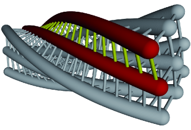
Figure 1: Wormlike bundle model. We consider bundles that consist of regular arrangements of filament. These are assumed to be locked in place by crosslinking proteins. When the bundle bends and twists in space, the filaments start to slide along each other. This effect leads to shear deformation in the crosslinks.

These intriguing mechanical properties can be understood in terms of the wormlike bundle model (WLB), which describes bundles as an assembly of semiflexible filaments interconnected by crosslinking proteins Bathe et al. (2008); Heussinger et al. (2007); for an illustration of the bundle architecture see Fig. 1. Unlike the standard wormlike chain model (WLC) Kratky and Porod (1949); Saitô et al. (1967), the wormlike bundle model (WLB) exhibits a state-dependent bending stiffness Bathe et al. (2008) that derives from a generic competition between the bending and twist stiffness of individual filaments and their relative motion mediated by the stiffness of the crosslinkers. An important aspect of the WLB model is that crosslinks may be very efficient in constraining the lateral excursions of filaments within the bundle but much less so in inhibiting their axial motion. This is possible as the relative axial sliding of two crosslinked filaments probes not only the elastic properties of the crosslinking protein but also those of the binding domain at which the protein is attached to the filament. The latter may be of quite different rigidity than the protein itself. Unfortunately there are no single-molecule experiments yet which would quantify the mechanical and binding properties of actin crosslinking proteins attached to a pair of F-actin filaments . In the WLB model the mechanical properties of the crosslinks are described by a single shear-stiffness $k_{\times}$ for the relative sliding of the constituent filaments.

An important finding within the wormlike bundle model is that the mechanical properties of bundles can be classified into three distinct bending regimes that are mediated by both crosslink type and equally importantly by bundle dimensions, namely diameter and length  Bathe et al. (2008). Taking into account the mechanical properties of filaments and crosslinker at a microscopic level is a virtue of the model making it quite verstile. It reduces to a well defined continuum limit but is equally applicable to bundles with as few as two filaments. This microscopic perspective may prove a valuable starting point to address more complex questions related to bundle mechanical properties. This may include problems such as disorder, lattice defects Gov (2008), or filament fracture Guild et al. (2003).

While previously we have provided a formulation only for plane-bending in two dimensions Heussinger et al. (2007), here we give a full derivation of the WLB Hamiltonian in three spatial dimensions. This includes bending as well as twist deformations. We explore the predictions of the WLB model for experimental observables such as the tangent-tangent correlation function and dynamic response functions. Moreover, we discuss the effects of different bundle geometries on their mechanical properties. In this respect, we will view microtubules as a bundle of (proto-)filaments arranged on the surface of a cylinder; compare Fig. 2. This shell-like bundle architecture is contrasted with a uniform distribution of filaments as found for F-action bundles Claessens et al. (2008); Purdy et al. (2007). Finally, we discuss how helicity influences bundle mechanics.

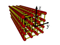
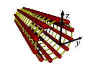
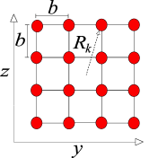
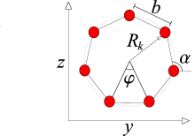
Figure 2: llustration of the bundle geometries considered. The position of the $k$th filament in the cross-sectional plane ($(y,z)$-plane) is given by ${\bf R}_{k}$. F-actin bundle architecture (left): filaments are arranged on a square lattice. Microtubule architecture (right): filaments are arranged on the surface of a cylinder.

II Model definition

We consider bundles of length $L$ that consist of $N$ parallel filaments. While the filaments may form a disordered lattice structure, we will focus our attention here to the cases of regular arrangements. In particular we will treat in detail the square-lattice and the cylindrical tube (see Fig. 2).

Each filament is modeled mechanically as an extensible worm-like polymer with stretching stiffness $k_{s}$, bending rigidity $\kappa_{b}$ and twist rigidity $\kappa_{t}$. Filaments are irreversibly crosslinked to their nearest-neighbors by crosslinks with mean axial spacing $\delta$. The crosslinks are modeled to be compliant in shear along the bundle axis with finite shear stiffness $k_{\times}$, and to be inextensible transverse to the bundle axis, thus constraining the interfilament distance, $b$, to be constant (see Fig. 2). This assumption, which neglects crosslink stretching deformations, is based on the recognition that the shearing mode involves deformation of the crosslink and its binding domain to the filament. The resulting stiffness may indeed be much lower than that of a crosslink in isolation.

Filament stretching is characterized by the axial displacement $u_{k}(s)$ of filament $k$ at axial position $s$ along the backbone. To describe bundle bending and twisting we define $\{\mathbf{d}_{1},\mathbf{d}_{2},\mathbf{d}_{3}\}$ to be a material frame fixed to the bundle central line at each arclength position $s$. The vector $\mathbf{d}_{3}\equiv\mathbf{t}$ is the tangent to the space curve traced out by the central line, while the two vectors $\mathbf{d}_{1}$ and $\mathbf{d}_{2}$ lie within the cross-section of the bundle. The position of each filament in the cross-section is parametrized in terms of a vector $\mathbf{R}_{k}(s)=A_{k}\mathbf{d}_{1}(s)+B_{k}\mathbf{d}_{2}(s)$, where $A_{k}$ and $B_{k}$ are the material-frame coordinates of filament $k$; they are constants independent of arclength $s$ and deformation of the central line (see Fig. 2). As one moves along the bundle backbone the material frame rotates according to Frenet-Seret equations, $\partial_{s}\mathbf{d}=\mathbf{\Omega}\times\mathbf{d}$. The rate of rotation is given by the generalized curvatures $\mathbf{\Omega}=(\Omega_{1}(s),\Omega_{2}(s),\Omega_{3}(s))$, which, in addition to the axial displacement $u_{k}$, represent the basic kinematic degrees of freedom of the bundle.

II.1 The WLB Hamiltonian

Neglecting all nonlinear effects we are now going to develop a simple expression for the bundle energy which is harmonic in its degrees of freedom, axial displacement $u_{k}$ and generalized curvatures $\Omega_{\alpha}$.

This WLB Hamiltonian consists of three contributions, $H_{\rm WLB}=H_{\rm 0}+H_{\rm stretch}+H_{\rm shear}$. The first term corresponds to the standard wormlike-chain Hamiltonian

$$H_{0}=\frac{N}{2}\int_{0}^{L}ds\left[\kappa_{b}\left(\Omega_{1}^{2}+\Omega_{2}^{2}\right)+\kappa_{t}\Omega_{3}^{2}\right]\,.$$ (1)

Writing this we assume that each filament follows effectively the same space-curve as the center-line. While, in general, one should account for the curvatures, $\mathbf{\Omega}_{k}$, of each individual filament separately, this would only lead to correction factors that can be neglected for our purposes. Consider, for example, planar bending of the central line, $\Omega_{1}=1/\rho$, where $\rho$ is the radius of curvature. The filaments that lie at a distance $R$ away from the central line naturally have a different radius of curvature, $\rho\pm R$, and thus a different bending energy. The magnitude of the correction term relative to $\Omega_{1}^{2}$ is small since it scales as $(R/\rho)^{2}$, i.e. we assume the typical curvatures to be smaller than the bundle radius (for more details see Appendix B).

As to the twist degree of freedom, in Eq. (1) we do not allow for the possibility of relative twisting of the individual filaments (see Section V and Appendix B for a discussion of this effect). We assume that twist is only due to the “bundle-twist” $\Omega_{3}$ of the central line. This assumption is reasonable in tightly bound bundles, where the filaments are connected by many crosslinks. In this state the filaments and their relative orientation can be assumed to be locked-in by the crosslinker.

The second term in the Hamiltonian, $H_{\rm stretch}=\sum_{k}H_{\rm stretch}^{k}$, accounts for filament stretching. It depends on the difference in axial displacement, $u_{k}$, between two crosslinks at arclength positions $s_{i}$ and $s_{i}+\delta$, respectively.

$$H_{\rm stretch}^{k} = \frac{k_{s}}{2}\sum_{i}\left[u_{k}(s_{i}+\delta)-u_{k}(s_{i})\right]^{2}$$ (2)

$$\to \frac{k_{s}\delta}{2}\int_{0}^{L}ds\left(\frac{\partial u_{k}}{\partial s}\right)^{2}\,,$$

where we have performed the continuum limit $\sum_{i}\to\int ds/\delta$ to arrive at the second line. The spring constant $k_{s}(\delta)$ is the single filament stretching stiffness on the scale of the crosslink spacing $\delta$.

The particular form for $k_{s}$ depends on the system under consideration. For high crosslink concentrations (small $\delta$), the segment behaves as a homogeneous elastic beam, characterized by a Youngs modulus $E$ and $k_{s}^{\rm beam}\sim Eb^{2}/\delta$. The combination $k_{s}\delta$ that enters the Hamiltonian is independent of $\delta$, as it should: the mechanical stretching stiffness of a beam cannot depend on the properties of the crosslinks.

For small concentrations of crosslinks (large $\delta$) entropic effects become relevant and the stretching stiffness is that of a thermally fluctuating wormlike chain with persistence length $l_{p}$. In this case one has $k_{s}^{\rm entr}\sim\kappa_{b}l_{p}/\delta^{4}$, which implies that the combination $k_{s}\delta\sim\delta^{-3}$ does depend on the crosslink spacing $\delta$. This is related to the fact that the formation of a crosslink suppresses thermal undulations (reduces entropy) and thus increases the entropic stretching stiffness. Equating both stretching stiffnesses, $k_{s}^{\rm beam}\sim k_{s}^{\rm entr}$ one finds the critical crosslink concentration, $\delta_{c}^{3}\sim b^{2}l_{p}$, at which the cross-over from enthalpic to entropic elasticity takes place.

In the case of microtubules, which will be treated in Section IV, the crosslink spacing $\delta$ is given by the tubulin-size and the stretching stiffness is modeled as for an elastic beam.

The third energy contribution, $H_{\rm shear}=\sum_{lk}H_{\rm shear}^{lk}$, results from the crosslink-induced coupling of neighboring filaments. The relative axial motion of a filament pair $(l,k)$ at a given point of the backbone is described by the crosslink shear displacement, which is the sum of a geometric contribution, $\Delta_{lk}$, and the relative stretching of neighboring filaments, $\Delta u_{lk}=u_{l}-u_{k}$. The geometric part results from the arclength mismatch between the two filaments, induced by a bending and twisting of the bundle central line. As in Eq. (2) we first write the shear energy as a sum over all crosslink positions $s_{i}$ and then perform the continuum limit, to get

$$H_{\rm shear}^{lk} = \frac{k_{\times}}{2}\sum_{i}\left[\Delta_{lk}(s_{i})+\Delta u_{lk}(s_{i})\right]^{2}$$ (3)

$$\to \frac{k_{\times}}{2\delta}\int_{0}^{L}ds\left(\Delta_{lk}+\Delta u_{lk}\right)^{2}\,,$$

where $k_{\times}$ is the shear stiffness of the individual crosslink.

For any bundle deformation, the associated value of $\Delta_{lk}$ can be compensated for by stretching the filaments, making the shear energy vanish when $\Delta u_{lk}=-\Delta_{lk}$. At the same time, however, this would increase the stretching energy, which may be unfavorable if the stretching stiffness $k_{s}$ is rather large. For deformations on the scale of the bundle length ($u^{\prime}\sim u/L$) the ratio of both energies gives the important parameter $\alpha=k_{\times}L^{2}/k_{s}\delta^{2}$, which quantifies the relative strength of both deformation modes Bathe et al. (2008).

As a final ingredient to the model we need to calculate the dependence of $\Delta_{lk}$ on the bundle curvatures, $\Omega_{\alpha}$. Without going into the details of an explicit derivation, we here just give the resulting expression. For more details we refer the reader to Appendix C. The special case relevant for the microtubule geometry is also dealt with in some detail in Hilfinger and Jülicher (2008). To linear order in $\Omega_{\alpha}$ we find

$$\Delta_{lk} = b_{lk}\cos\alpha_{lk}\left(y_{lk}\Omega_{3}-\int_{0}^{s}dt\Omega_{2}(t)\right)$$

$$-b_{lk}\sin\alpha_{lk}\left(z_{lk}\Omega_{3}-\int_{0}^{s}dt\Omega_{1}(t)\right)\,,$$

where we defined $b_{lk}=|\mathbf{b}_{lk}|$ as the distance between the filament pair and $\alpha_{lk}$ as the angle of $\mathbf{b}_{lk}$ with respect to the $z$-axis. Furthermore, $(y_{lk},z_{lk})$ are defined as the cross-sectional coordinates of the midpoint between the filament pair.

In contrast to $H_{0}$, which is an expansion in the generalized curvatures $\Omega_{\alpha}$, the shear energy $H_{\rm shear}$ is a function of the integrated curvatures, since $\Delta\sim b\int_{s}\Omega\sim bL\Omega$. For terms beyond the harmonic contribution to be negligible, one has to assume that the shear displacement is sufficiently small, $\Delta\ll a$, where $a$ is some microscopic length-scale related to the size of the crosslink. In terms of the bundle curvatures this implies $L\Omega\ll a/R\sim 1$, which is much more restrictive than the range $R\Omega\ll 1$, over which $H_{0}$ can be approximated by a harmonic form. As a consequence the bundle is only allowed to make small excursions from its initial state, an assumption which is usually well satisfied in bundles of stiff polymers like actin or microtubules, but certainly breaks down under extreme loading conditions (e.g. to describe post-buckling) or in more flexible objects like DNA.

With this “weakly-bending” assumption we reformulate the generalized curvatures in terms of the lab-frame Euler angles Alim and Frey (2007); Goldstein et al. (2002)

$$\Omega_{1} = \frac{\partial\phi}{\partial s}\sin\psi\sin\theta+\frac{\partial\theta}{\partial s}\cos\psi$$

$$\Omega_{2} = \frac{\partial\phi}{\partial s}\cos\psi\sin\theta-\frac{\partial\theta}{\partial s}\sin\psi$$

$$\Omega_{3} = \frac{\partial\psi}{\partial s}+\frac{\partial\phi}{\partial s}\cos\theta\,.$$

As reference state we take $\phi_{0}=\pi/2$, $\theta_{0}=\pi/2$ and $\psi_{0}=s\omega_{0}$, which corresponds to a straight, but pre-twisted bundle that points along the $x$-axis. For small excursions around this reference state we can linearize the equations such that

$$\Omega_{1} = \frac{\partial\phi}{\partial s}\sin\psi_{0}+\frac{\partial\theta}{\partial s}\cos\psi_{0}$$ (5)

$$\Omega_{2} = \frac{\partial\phi}{\partial s}\cos\psi_{0}-\frac{\partial\theta}{\partial s}\sin\psi_{0}$$

$$\Omega_{3} = \frac{\partial\psi}{\partial s}\,,$$

and the angles are now measured relative to the reference state. As expected the pretwist $\psi_{0}$ leads to a coupling of the angles $\theta$ and $\phi$. In the following we are primarily concerned with the case of vanishing pretwist. Then, the coupling terms vanish and we can simply set

$$(\Omega_{1},\Omega_{2},\Omega_{3})=(\theta^{\prime},\phi^{\prime},\psi^{\prime})\,.$$

We will come back to the case of pretwist in Section V.

II.2 Examples for the arclength mismatch $\Delta$

For the purpose of illustration we provide some examples of how the shear displacement $\Delta$ depends on the geometry of the bundle cross-section and the deformation of its central line.

If the bundle consists of only two filaments Everaers et al. (1995) (geometry of a ribbon) we have $y=z=\alpha=\pi/2$ as the central line and the mid-line between the two filaments are identical. In this case $\Delta$ simplifies to

$$\Delta=b\theta(s)\,,$$ (6)

which is illustrated in Fig. 3. Note, that twist ($\Omega_{3}$) does not contribute, as both filaments twist around the central line symmetrically.

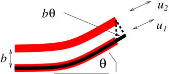
Figure 3: Illustration of crosslink shear deformation for the case of a two-filament bundle (filaments in red). Bundle deflection through the angle $\theta$ leads to the arclength mismatch, $\Delta=b\theta$. The filaments have to stretch the relative amount $u_{1}-u_{2}=b\theta$, in order to keep the crosslink (dashed line) undeformed with zero shear energy.

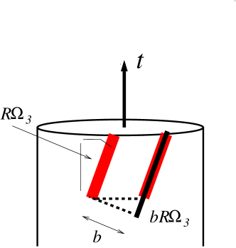
Figure 4: Illustration of crosslink shear deformation for a twisted microtubule. Indicated (in red) is a filament pair that winds around the microtubule cylinder (radius $R$) taking an angle $R\Omega_{3}$ with the cylinder axis $\mathbf{t}$. The resulting arclength mismatch is given by $\Delta=bR\Omega_{3}$.

A particular case of this two-filament bundle has been considered in a set of articles Mergell et al. (2002); Golestanian and Liverpool (2000); Zhou et al. (2000), where the crosslinks are assumed to be rigid with respect to shear, i.e. $k_{\times}\to\infty$. To satisfy a vanishing arclength mismatch $\Delta$ one thus requires $\Omega_{1}\equiv-\mathbf{d}_{2}^{\prime}\cdot\mathbf{t}=0$. This means that the unit vector $\mathbf{d}_{2}$, which points from one filament to the other, must not rotate in the direction of the tangent $\mathbf{t}$. In other words, $\mathbf{d}_{2}$ must equal the the bi-normal. Thus the ribbon orientation is completely specified by the space curve traced by the central line.

A second example is the axoneme in eukaryotic flagellae Hilfinger and Jülicher (2008). There, filaments (microtubule doublets) are arranged on the surface of a cylinder, just as the protofilaments in a single microtubule. Switching to polar coordinates in the cross-sectional plane (see Fig. 2), $(y,z)\to(R,\varphi)$, $\alpha=\varphi+\pi/2$, we find

$$\Delta=-bR\psi^{\prime}+b\phi\sin\varphi+b\theta\cos\varphi\,.$$ (7)

A similar expression, disregarding the possibility of twisting, has been given by Mohrbach et al. Mohrbach and Kulic (2007). The structure of the second and third term is the same as in Eq. (6), additionally taking into account the modified orientation in the cross-sectional plane, as described by the angle $\varphi$. The origin of the first term is illustrated in Fig. 4 and elaborated on in Appendix C.

Consider now the case of planar bending. This will make the connection to continuum elasticity particularly clear. Under planar deformation the bundle is described by the one variable $\theta^{\prime}=\Omega$ such that the shear deformation is simply $\Delta=b\theta(s)\sim b\partial_{x}u_{y}$. Here, $u_{y}$ is the displacement of the bundle transverse to the bundle axis (in the y-direction). This latter form makes clear that the shear deformation represents one part of the strain tensor component $\epsilon_{xy}=\frac{1}{2}(\partial_{x}u_{y}+\partial_{y}u_{x})$. The second part, $\partial_{y}u_{x}\sim b\Delta u_{lk}$ is the continuum version of relative filament stretching (see Eq. (3)).

The elastic symmetries relevant to the WLB model depend on the arrangement of the filaments in the cross-section. If there is rotational symmetry with respect to the bundle axis, one speaks of transversly isotropic elastic bodies Love (1944). While, in general, this has five first order elastic constants, our model has only two, augmented by the (second order) bending/twisting elasticity of the individual filaments which is not accounted for in continuum elasticity. The simplification arises from assuming transverse inextensibility as well neglecting cross-sectional shape changes. The latter is, for example, important in the failure of hollow tubes under bending. One relevant effect is the Brazier effect Calladine (1983), which describes the increasing ovalization of the cross-section under the action of a bending moment. In the present formulation of the model these nonlinearities are not accounted for. For a discussion of potential modifications to include cross-sectional deformations, we refer the reader to the outlook section at the end of this article.

II.3 Definition of effective bending and twist rigidities

It should be clear from the way the Hamiltonian was derived that the model is applicable to bundles with arbitrary (ordered/disordered) arrangements of filaments in the cross-section. In the remainder of this article we will focus our attention to bundles with highly symmetric cross-sections, where the filaments either form a rectangular array or a hollow tube.

In view of recent experiments probing the mechanical or statistical properties of individual bundles in vitro Claessens et al. (2006), we head at a description of the bundle in terms of effective bending and twist rigidities. These are defined with respect to the standard worm-like chain model. To arrive at the proper expressions we have to integrate out the internal stretching variable $u$, which in general is not observable in experiment.

To show how this works, we symbolically write the partition function as $Z=\int D\boldsymbol{\phi}Z(\boldsymbol{\phi})$ where $\boldsymbol{\phi}$ signifies the set of Euler angles $\phi(s),\theta(s),\psi(s)$. The constrained partition function then reads $Z(\boldsymbol{\phi})=\int D\{u\}\exp(-\beta H(\{\boldsymbol{\phi},u\}))\equiv\exp(-\beta W(\boldsymbol{\phi}))$.

The integration over the $u$-variables can easily be performed. As the Hamiltonian is harmonic we are left with only Gaussian integrals, which are evaluated in Fourier space. The resulting potential of mean force $W(\boldsymbol{\phi})$ can be written in the form of a wormlike chain Hamiltonian

$$W(\boldsymbol{\phi}_{n})=\frac{L}{4}\sum_{n}q_{n}^{2}\left[\kappa_{B}(n)(\phi_{n}^{2}+\theta_{n}^{2})+\kappa_{T}(n)\psi_{n}^{2}\right]$$ (8)

with effective bending and twist rigidities $\kappa_{B}(n)$ and $\kappa_{T}(n)$, respectively. We note that in the symmetric situations considered here there is no coupling between the different deformation modes bending and twisting (see Appendix A). In contrast to the usual WLC, the effective bend and twist rigidities are in general dependent on the mode-number $n$ and thus on the wavelength of the deformation. This effect and the discussion of its consequences is the central topic of the remaining sections.

III F-Actin bundle architecture

In the following sections we will focus our attention to bundles with $N=(2M)^{2}$filaments that form a rectangular array (see Fig. 2). The angle $\alpha$ that specifies the orientation of the filament-pair in the cross-section is then $\alpha=0,\pi/2$ as filaments are either arranged along the $y$- or the $z$-axis. As mentioned above the different deformation modes decouple in harmonic order. We can thus investigate bending independently from twisting. Also the two space-directions decouple and we can reduce the model to an effective two-dimensional description Heussinger et al. (2007).

III.1 Effective bending rigidity

The shear Hamiltonian reduces to

$$H_{\rm shear}=\frac{Mk_{\times}}{\delta}\int_{0}^{L}\!ds\sum_{k=-M+1}^{M-1}(u_{k+1}-u_{k}+b\theta)^{2}\,,$$ (9)

where we used Eq. (II.1) with $\phi=\psi=0$. By following the recipe outlined above we eliminate the axial strain variable $u_{k}$. By approximating $u_{k}$ by a linearly increasing function of $k$ (see discussion below) we arrive at the following result for the effective bending rigidity  as defined in Eq. (8)

$$\kappa_{B}(n)=N\kappa_{b}\left[1+\left(\frac{12\hat{\kappa}_{b}}{N-1}+(q_{n}\lambda)^{2}\right)^{-1}\right]\,.$$ (10)

Here, we have defined a characteristic wavelength

$$\lambda=\sqrt{\frac{2M}{(2M-1)}}\cdot\sqrt{\frac{\kappa_{b}\delta}{k_{\times}b^{2}}}\,,$$ (11)

and a dimensionless bending rigidity $\hat{\kappa}_{b}=\kappa_{b}/(k_{s}\delta b^{2})$. In terms of the quantities $\lambda$ and $\hat{\kappa}_{b}$ the previously defined $\alpha=k_{\times}L^{2}/k_{s}\delta^{2}$ can be rewritten as $\alpha\sim\hat{\kappa}_{b}(L/\lambda)^{2}$. If the filaments behave as homogeneous elastic beams, $\hat{\kappa}_{b}$ is just a number independent of bundle geometry or crosslink spacing. For any numeric computation we will, for specifity, assume that $\hat{\kappa}_{b}=1/12$, which corrresponds to beams with square cross-sections Landau and Lifschitz (1970).

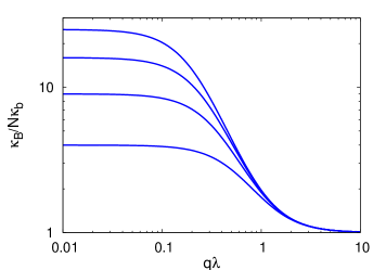
Figure 5: Effective bending rigidity, Eq. (10), as a function of mode-number, $q\lambda$, and for the set of bundle sizes $N=4,9,16,25$ (from bottom to top). In the fully-coupled and the decoupled regimes (corresponding to small and large $q$) the bending rigidity is constant. At intermediate values of $q$ the bending rigidity scales as $\kappa_{B}(n)\sim k_{\times}q_{n}^{-2}$ (shear-dominated regime).

The characteristic feature of Eq. (10), is the wavelength dependence (see Fig. 5). For wavelengths $q_{n}^{-1}$ in the interval $1/\sqrt{N}\ll q_{n}\lambda\ll 1$ the bending stiffness decreases as $\kappa_{B}(n)\sim k_{\times}q_{n}^{-2}$. In Ref. Bathe et al. (2008) we have termed this the intermediate or shear dominated regime as the bending rigidity is proportional to the shear stiffness of the crosslinks. It is in this parameter regime that the bundle behaves qualitatively different than either a homogeneous beam (obtained in the ”fully coupled” limit of $q_{n}\lambda\ll 1/\sqrt{N}$) or an assembly of ”decoupled” filaments ($q_{n}\lambda\gg 1$).

Another important feature of Eq. (10), which is independent of the specific $q$-dependence, is the ratio of maximal to minimal bending rigidity, $r=\kappa_{\max}/\kappa_{\min}=1+(N-1)/12\hat{\kappa}_{b}$. This only depends on the number of filaments and the dimensionless bending rigidity $\hat{\kappa}_{b}$.

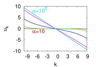
Figure 6: Dependence of axial strain $u_{k}$ on $k$, the distance from the bundle central line. Decreasing the dimensionless shear-stiffness $\alpha=k_{\times}L^{2}/k_{s}\delta^{2}$ the strain is reduced but not in a linear fashion. The outer layers of the bundle remain stretched stronger than the inner ones.

While integrating out the stretching variables $u_{k}$ can be performed exactly, Eq. (10) is based on the additional assumption that axial strains are linearly increasing through the cross-section, $u_{k}=\Delta u\cdot(k+1/2)$. The exact profile for $u_{k}$ is calculated in the appendix and displayed in Fig. (6); compared to the linear profile it shows an enhancement of strain towards the bundle periphery.

However, the ensuing value for the bending stiffness is largely insensitive to the linear approximation . We speculate that the nonlinearities in the axial strain may eventually be important for nonlinear material properties, as for example strain induced rupture. The increased strain in the outermost filaments brings them closer to their threshold for rupture and thus makes them more susceptible to this mode of failure.

In order to make contact with continuum models for beam bending we perform a continuum limit, by letting $N\to\infty$ but keeping the bundle aspect ratio $D/L\sim bM/L$ constant. Then, bundle length $L$ has to grow with $M$ as $L(M)\sim M$. In particular, this implies that fewer and fewer modes $n$ belong to the decoupled regime (where $q_{n}^{-1}\ll\lambda$). Eventually, this regime, where filaments bend independently ($\kappa_{B}(n)\approx N\kappa_{b}$) is no longer accessible. In effect this means that the bending stiffness $\kappa_{b}$ of the individual filaments can be neglected, just as in ”normal” continuum elasticity, where higher order gradients (${\cal O}(\theta^{\prime})$) are not accounted for from the start.

In this continuum limit the result from the linearization assumption, Eq. (10), reduces to the Timoshenko model for beam bending Gere and Timoshenko (2002), which was recently used to interpret bending stiffness measurements on microtubules Kis et al. (2002); Pampaloni et al. (2006) and carbon nanotube bundles Kis et al. (2004),

$$\kappa_{B}^{\rm TIMO}(n)=\frac{N^{2}\kappa_{b}}{1+(q_{n}D)^{2}E/12G}\,.$$ (12)

To allow for comparison with continuum elasticity we have used the expressions $k_{s}\delta=Eb^{2}$ and $\kappa_{b}=Eb^{4}/12$ applicable for homogeneous beams of square cross-section and defined the shear-modulus $G=k_{\times}/\delta$.

On the other hand, one can equally derive a continuum limit from the exact expression for $\kappa_{B}(n)$ (as presented in Appendix A.1). This gives

$$\kappa_{B}^{\rm CONT}(n)=\frac{N^{2}\kappa_{b}}{(q_{n}D)^{2}E/12G}\left(1-\frac{\tanh(q_{n}D\sqrt{E/4G})}{q_{n}D\sqrt{E/4G}}\right)\,.$$ (13)

Both expressions, Eq. (12) and Eq. (13) are compared in Fig. (7). One infers that the approximation (Timoshenko theory) overestimates the exact solution by no more than $6\%$. The difference can partly be compensated for by introducing a shear-correction factor ($\approx 1.2$) in the denominator of Eq. (12).

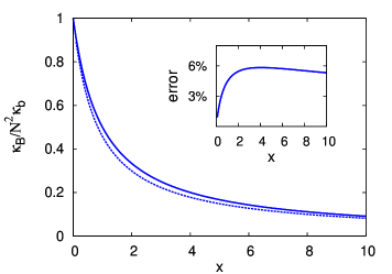
Figure 7: Continuum limit of effective bending rigidities as a function of $x=(q_{n}D)^{2}E/12G$. Comparison of exact solution, Eq. (13), with approximation, Eq. (12). Inset: Relative error between both expressions. The approximation over-estimates the bending stiffness by maximal $\sim 6\%$.

III.2 Tangent-tangent correlation function

In this section the implications of a mode-number dependent bending rigidity is further elaborated by discussing the concept of the persistence length. The persistence length of a single WLC may be defined in terms of the competition of bending and thermal energies, $l_{p}=\kappa/k_{B}T$. With this definition, bending rigidity and persistence length are basically identical. In the framework of the WLB this would lead to a mode-number dependent persistence length $l_{p}(n)=\kappa_{B}(n)/k_{B}T$.

For the WLC the persistence length is also the length-scale over which the tangent-tangent correlation function decays

$$\langle\mathbf{t}(s)\mathbf{t}(0)\rangle=\exp\left[-s/l_{p}\right]\,.$$ (14)

This simple exponential form is no longer valid for the WLB as can be illustrated by considering planar bending with $\phi=0$. Then the tangent-tangent correlation function is easily inferred from the angular fluctuations Everaers et al. (1995) as

$$\langle\mathbf{t}(s)\mathbf{t}(0)\rangle=\exp\left[-\frac{1}{2}\left\langle\left(\theta(s)-\theta(0)\right)^{2}\right\rangle\right]\,,$$ (15)

with

$$\left\langle\left(\theta(s)-\theta(0)\right)^{2}\right\rangle=\frac{1}{Nl_{p}}\left[\frac{A-1}{A}s+\frac{\displaystyle\lambda}{\displaystyle A\sqrt{A}}\left(1-e^{-s\sqrt{A}/\lambda}\right)\right]\,,$$ (16)

and $A=1+12\hat{\kappa}_{b}/(N-1)$. Forcing such a complex expression into the form given by Eq. (14) implies an arclength-dependent persistence length, $l_{p}(s)$. At short distances, one recovers the decoupled regime and $l_{p}(s)=Nl_{p}$, while at long distances, $l_{p}(s)=N^{2}l_{p}$ as found in the fully coupled regime.

Note, that there is no immediate relation between this $l_{p}(s)$ and the $l_{p}(n)$ defined above. The Fourier-transform of $l_{p}(n)$ is, instead, given by the following expression

$$l_{p}^{\star}(s)=\frac{N\kappa_{b}}{k_{B}T}\left(L\delta(s)+\frac{L}{\lambda}\frac{e^{-\sqrt{A-1}s/\lambda}}{\sqrt{A-1}}\right)\,.$$ (17)

This quantity appears in the elastic energy expressed in real-space as

$$H_{\rm WLB}=k_{B}T\int\theta^{\prime}(s_{1})l_{p}^{\star}(s_{1}-s_{2})\theta^{\prime}(s_{2})ds_{1}ds_{2}\,,$$ (18)

which is a non-local function of arclength. The length-dependence obtained here is markedly different from that found in the correlation function, Eq. (16). While $l_{p}(s)$ is constant at large distances, $l_{p}^{\star}(s)$ decays exponentially and vanishes over the length-scale $\lambda/\sqrt{A-1}\sim\lambda\sqrt{N/\hat{\kappa}_{b}}$, which corresponds to the onset of the fully-coupled regime.

A similar nonlocal energy function is obtained when considering the fluctuation properties of elastic membranes. In-plane shear- and compression-modes lead to a renormalized bending rigidity for the out-of-plane fluctuations Nelson and Peliti (1987); Nelson et al. (2004). In contrast to bundles, however, there the kernel is long-ranged $\l_{p}(s)\sim 1/s$, which asymptotically leads to a flat membrane phase.

Concluding this section, we find that it is impossible to speak of a single persistence length without specifying the precise experimental conditions as well as the observable under consideration (here tangent-tangent correlation function). The WLB model presents a framework within which a length-dependent bending stiffness can be understood. However, we would like to emphasize that the fundamental quantity is the $q_{n}$-dependent $\kappa_{B}(n)$ as presented in Eq. (10) or below in Eq. (26). It depends on wavenumber in a universal way independent of the type of measurement. The dependence on bundle length, in contrast, arises through a specific transformation to real space and may produce different results depending on the observable under consideration.

III.3 Frequency-dependent correlation and response functions

In our previous publications Bathe et al. (2008); Heussinger et al. (2007) we have calculated several thermodynamic observables and showed that the mode-dependent bending stiffness of a WLB may lead to drastic modifications of their scaling behavior. Here, we widen the scope of this analyis by discussing dynamic observables. In analogy to the usual overdamped dynamics of a WLC we can discuss the dynamics of a WLB by substituting the mode-dependent bending stiffness in the standard Langevin equation of motion for the transverse bending modes $r_{\perp}(q_{n},t)$

$$\zeta\frac{\partial r_{\perp}}{\partial t}=-\kappa_{B}(n)q_{n}^{4}r_{\perp}+\xi(q_{n},t)\,.$$ (19)

With this one obtains for the reduced correlation function

$$C(t) := L^{-1}\int_{0}^{L}\left\langle\left(r_{\perp}(s,t)-r_{\perp}(s,0)\right)^{2}\right\rangle ds\,.$$ (20)

$$= \frac{k_{B}T}{L}\sum_{n}\frac{1-e^{-t/\tau_{n}}}{\kappa_{B}(n)q_{n}^{4}}\,,$$

with the relaxation times $\tau_{n}=\zeta/\kappa_{B}(n)q_{n}^{4}$. For WLCs (constant $\kappa_{B}\equiv\kappa$) one finds a scaling regime at times $t<\tau_{1}\sim\zeta L^{4}/\kappa$, where $C(t)\sim t^{3/4}$ Frey and Nelson (1991); Kroy and Frey (1997); Isambert and Maggs (1996).

For WLBs, on the other hand, one has to use the $q$-dependent effective bending stiffness, Eq. (10), instead. As the term $(q\lambda)^{-2}$ multiplies the $q^{4}$ contribution in Eq. (20) one finds the correlations to grow in time as $C_{\rm WLB}(t)\sim t^{1/2}$. Of course, this result is only valid as long as the $q\lambda$-term dominates the effective bending stiffness, i.e. as long as the bundle is in the intermediate regime. In fact, there will be a complex cross-over scenario

$$C(t)\sim\begin{cases}(Nl_{p})^{-1}\left(\dfrac{N\kappa_{b}t}{\zeta}\right)^{3/4}\,,&\text{$t\ll t_{1}$}\\ (Nl_{p})^{-1}\lambda^{2}\left(\dfrac{N\kappa_{b}t}{\zeta}\right)^{1/2}\,,&t_{1}\ll t\ll t_{2}\\ (Nl_{p})^{-1}\left(\dfrac{\hat{\kappa}_{b}}{N}\right)^{1/4}\left(\dfrac{N\kappa_{b}t}{\zeta}\right)^{3/4}\,,&\text{$t_{2}\ll t\ll t_{3}$}\\ (Nl_{p})^{-1}L^{3}\dfrac{\hat{\kappa}_{b}}{N}\,,&\text{$t\gg t_{3}$}\end{cases}$$ (21)

with the cross-over times $t_{1}=\zeta\lambda^{4}/N\kappa_{b}$ and $t_{2}=t_{1}\dfrac{\hat{\kappa}_{b}}{N}$ governing the cross-over from the decoupled to the intermediate and the fully-coupled regimes. At times larger than $t_{3}=t_{1}\dfrac{\hat{\kappa}_{b}}{N}\dfrac{L^{4}}{\lambda^{4}}$ the correlation function saturates.

From the correlation function one can furthermore calculate the response function $\chi_{\perp}$ measuring the linear response to transverse forces. Using the fluctuation-dissipation theorem and the Kramers-Kronig relations one finds

$$\chi_{\perp}(\omega)=\sum_{n}\frac{1}{L}\frac{1}{\kappa_{B}(n)q_{n}^{4}-i\zeta\omega}\,.$$ (22)

This contrasts with the response function $\chi_{\parallel}$ for stretching forces

$$\chi_{\parallel}(\omega)=\sum_{n}\frac{1}{l_{p}(n)}\frac{1}{\kappa_{B}(n)q_{n}^{4}-i\zeta\omega/2}\,,$$ (23)

which is sometimes taken as a starting point to determine the high-frequency response of entangled solutions of stiff polymers Gittes and MacKintosh (1998); Morse (1998a, b); Granek (1997); Koenderink et al. (2006), The transverse response, on the other hand, has been argued to relate to a “microrheological modulus” Frey et al. (2000); Kroy and Glaser (2007) that is measured locally by imbedding probe beads into the network. Unfortunately, for a WLC both functions are hardly indistinguishable, and only differ by the constant factor $\chi_{\parallel}/\chi_{\perp}=L/l_{p}$. The high-frequency behavior in both cases is $\chi\sim\omega^{-3/4}$.

In the case of a WLB, things are somewhat different, as the additional factor $L/l_{p}(q)$ in the longitudinal response function not only changes the prefactor but also modifies the functional form with respect to frequency (see Fig. 8).

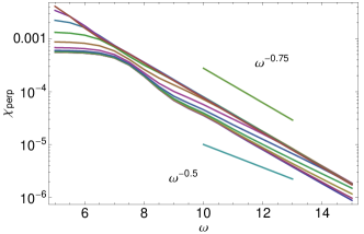
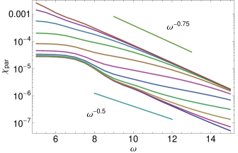
Figure 8: Comparison of transverse response function $\chi_{\perp}(\omega)$ (top) with longitudinal response function $\chi_{\parallel}(\omega)$ (bottom) for a bundle of $N=20$ filaments (in units of $N\kappa_{b}/L^{3}$ and assuming $Lk_{B}T/N\kappa_{b}=1$). Frequencies are plotted in units of $\zeta L^{4}/N\kappa_{b}$. The different curves correspond to different values of $\lambda/L$. The two asymptotic scaling regimes with $\omega^{-3/4}$ correspond to the decoupled (top) and fully-coupled regime (bottom), respectively. The intermediate $\omega^{-1/2}$ is sharper in $\chi_{\perp}$ than in $\chi_{\parallel}$ even though the latter function shows overall a stronger variation with frequency.

For similar reasons as in the discussion of the correlation function one expects an intermediate regime with $\omega^{-1/2}$, at least in the transverse response. This should lead to measurable signatures in microrheological experiments on bundled F-actin systems. Due to the additional $q$-dependence in the denominator, the longitudinal response, $\chi_{\parallel}$ shows a smooth cross-over between the two asymptotic regimes of fully-coupled and decoupled bending, as explained in the figure.

III.4 Effective twist rigidity

We now turn to the discussion of the twist mode. In this case the Euler angles $\phi$ and $\theta$ in Eq. (II.1) are zero such that the shear Hamiltonian reduces to

$$H_{\rm shear}=\frac{k_{\times}}{2\delta}\int_{0}^{L}\!ds\sum_{lk}\left(\Delta u_{lk}+bd_{lk}\psi^{\prime}\right)^{2}\,,$$ (24)

where we defined the geometric factor $d_{lk}=y_{lk}\cos\alpha_{lk}-z_{lk}\sin\alpha_{lk}$.

As may already be apparent from comparing Eq. (9) with Eq. (24) the stretching deformation $u$ couples differently to twist ($k_{\times}u\psi^{\prime}$) as to bending ($k_{\times}u\theta$). The difference being the additional derivative occuring in Eq. (24). Effectively this means that the resulting twist rigidity will not depend on mode-number $q_{n}$ but receive a constant correction to the single filament value $\kappa_{t}$.

Let us first assume that the filaments are inextensible. Then the $u$-terms in the Hamiltonian identically vanish and the effective twist rigidity can simply be read off from the terms multiplying $\psi^{\prime 2}$,

$$\kappa_{T} := N\kappa_{t}\left[1+\frac{N-1}{6}\left(\frac{\lambda_{t}}{b}\right)^{-2}\right]\,.$$ (25)

Here we have defined $\lambda_{t}:=\sqrt{2M/(2M-1)}\sqrt{\kappa_{t}\delta/k_{\times}b^{2}}$, which is similar to $\lambda$ defined above, with $\kappa_{b}$ substituted by $\kappa_{t}$. Unlike $\lambda$, however, it multiplies the constant length $b$, the lateral distance between neighboring filaments. As anticipated, there is no mode-number dependence.

By introducing bundle diameter $D$ and effective shear modulus $G$ (as in the discussion leading to Eq. (12)) the second term takes a form well known from continuum theory, $\sim GD^{4}$ Landau and Lifschitz (1970). Thus, we find an effective twist rigidity, Eq. (25), that just describes the simple additive superposition of two contributions, shear-induced rigidity (second term) and twist rigidity of the individual filaments (first term). In the continuum limit $N\to\infty$ the latter contribution can naturally be neglected as it only grows with $N$ as compared to the $N^{2}$ increase of the shear-induced rigidity.

Now we allow for finite axial displacements $u_{k}$. This is commonly referred to as cross-sectional warping; under twist deformations the bundle cross-sections do not stay plane but deform and acquire a curvature. Just as in the case of the bending rigidity, the exact solution for the twist rigidity only differs little from the foregoing simplified analysis. Some details about the derivation are presented in Appendix A.2. The resulting axial displacements $u_{k}$ can be found in Fig. (9) The classic solution of Saint-Venant Love (1944) is approached closer and closer for increasing the shear-stiffness $k_{\times}$.

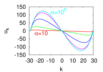
Figure 9: Cross-sectional warping $u_{k}$ ($k=-M+1\ldots M$, corresponding to one row of the rectangular array) for different non-dimensional crosslink shear stiffness $\alpha=k_{\times}L^{2}/k_{s}\delta^{2}$. The classic solution for a beam (dashed line) is approached as $k_{\times}\to\infty$. In the opposite limite, $k_{\times}\to 0$, there is no warping and $u\equiv 0$, as filaments remain uncoupled in this limit.

IV Microtubule architecture

In this section we want to turn our attention to the case of microtubules, which we model as bundles with filaments arranged on the surface of a cylinder. For the time being we assume that in the groundstate the microtubule is untwisted such that the $N$ protofilaments are oriented along the cylinder axis. This assumption is in fact only valid for microtubules with $N=13$ protofilaments Chrétien et al. (1992); Chrétien and Wade (1991). This class, nevertheless, seems to be the most frequent in in-vitro polymerization experiments.

There is an ongoing debate in the literature about the dependence of microtubule bending rigidity on length Kurachi et al. (1995); Kikumoto et al. (2006); Brangwynne et al. (2007); Pampaloni et al. (2006); Taute et al. (2008); van den Heuvel et al. (2008, 2007); Kis et al. (2002). Early buckling experiments indicated a length-dependence Kurachi et al. (1995), while an improved version of the same experiments later gave a negative result Kikumoto et al. (2006). Brangwynne et al. Brangwynne et al. (2007) performed a mode analysis of microtubule contours. Their data is compatible with a length-dependent bending rigidity but the authors vote for a cautious interpretation of the results in view of the close proximity to the noise level. Recently, experiments by Pampaloni et al. Pampaloni et al. (2006) measured the transverse fluctuations of grafted microtubules to establish an increasing persistence-length for microtubule lengths up to $L\sim 23\mu m$. Using a high-precision tracer technique, Taute et al. Taute et al. (2008) analyzed shorter microtubules and found the persistence length to level off at $l_{p}^{\rm min}\approx 580\mu m$ for lengths shorter than $L\approx 5\mu m$. Similar values have been obtained in Ref. van den Heuvel et al. (2008) ($l_{p}^{\rm min}=90\mu$m) and in Ref. van den Heuvel et al. (2007) ($l_{p}^{\rm min}=240\mu$m), and explained with the help of the WLB model. On short length-scales (in the decoupled regime) the effective bending rigidity is constant because it reflects the stiffness of the individual proto-filaments. In contrast, Kis et al. Kis et al. (2002) have found a decreasing bending stiffness even for microtubule sections as short as several hundred nanometers.

While the discussion about these partially conflicting measurements is ongoing, we would like to point out that different techniques do not necessarily have to come to the same conclusion, once the idea of the bending rigidity as a fundamental material parameter is given up. In the context of the WLB model the fundamental quantity is a mode-dependent bending rigidity. As discussed in Section III.2, any dependence on bundle length is a “secondary” effect that will depend on the observable under consideration.

By using the same procedure as in the case of the rectangular bundle we find for the microtubular bending rigidity

$$\kappa_{B}(n)=N\kappa_{b}\left[1+\left(\frac{8\hat{\kappa}_{b}}{\sin^{-2}(\pi/N)}+(q_{n}\lambda)^{2}\right)^{-1}\right]\,,$$ (26)

where the relevant length-scale $\lambda$ is now defined as $\lambda=\sqrt{\kappa_{b}\delta/k_{\times}b^{2}}$. Note, that this expression results in the bending stiffness in the fully-coupled regime (where the microtubule behaves as a simple beam) to scale as $\kappa\sim N^{3}$, in contrast to bundles with a homogeneous cross-section (as the one discussed before), where $\kappa\sim N^{2}$.

With Eq. (26) direct comparison with experimental data can be made. In particular, the ratio of maximal to minimal bending rigidity can most easily be determined, $r=1+\sin^{-2}(\pi/N)/8\hat{\kappa}_{b}=1+2/\sin^{2}(\pi/N)$. For the latter equality we assumed the protofilament to have a circular cross-section ($\hat{\kappa}_{b}=1/16$). For microtubules with $N=13$ protofilaments this results in a universal ratio $r\approx 35$.

In this way, using the the range of values $l_{p}^{\min}\approx 0.1\ldots 0.6$mm (which we assume to represent the protofilament stiffness) one can estimate the maximal persistence length of long microtubules to be in the range $l_{p}^{\max}\approx 3.5\ldots 21$mm. Compared with experiments Janson and Dogterom (2004); Gittes et al. (1994); Pampaloni et al. (2006) these values seem to be too large. Given the large error-bars in any of the mentioned experiments this calculation may, nevertheless, be acceptable. Furthermore, as we will discuss below, microtubule helicity can provide a mechanism to reduce the apparent persistence length by reducing the effect of shear-induced coupling. For given microtubule length the persistence length is then predicted to decrease with increasing helicity – thus improving the comparison with experiment.

Finally, let’s turn to the case of pure twist deformations. Due to the symmetry of the circular cross-section no warping is possible. We find for the microtubule twist rigidity, similar to Eq. (25),

$$\kappa_{T} := \kappa_{t}\left[1+\frac{\tan^{-2}(\pi/N)}{4}\left(\frac{\lambda_{t}}{b}\right)^{-2}\right]\,,$$ (27)

where $\lambda_{t}:=\sqrt{\kappa_{t}\delta/k_{\times}b^{2}}$.

V Pretwisted bundles

In the previous sections we have restricted our attention to non-helical bundles and assumed that in the ground-state the filaments point along the bundle axis. As a final application of our model, we will here discuss the question of helicity, or pretwist, and its influence on bundle mechanics. This aspect is important not only for some types of microtubules but also for F-actin bundles and is reflected in the role that helicity plays in providing an explanation for the existence of a (thermodynamically) preferred bundle size Grason and Bruinsma (2007); Grason (2009); Claessens et al. (2008).

The discussion of pretwisted bundles proceeds in two steps. We first assume the bundle to form with all filaments straight. Starting from this reference state crosslink binding may add a driving force for twisting the bundle if the straight state does not allow for optimal accessibility of the crosslink binding sites. Another effect may be the helicity of the filaments themselves that favor a twisted bundle over an untwisted one.

Without elaborating on the precise mechanism that leads to pretwisted bundles, we incorporate bundle pretwist by substituting the generalized twist-curvature $\Omega_{3}$ by $\Omega_{3}-\omega_{0}$. In doing so the new energetic ground-state is at $\Omega_{1}=\Omega_{2}=0$ and $\Omega_{3}=\omega_{0}$ . To obtain the effective bending rigidity we linearize the curvatures around this ground-state, as performed in Eq. (5).

Inserting this result into the shear deformation, Eq. (II.1), one finds terms like $b\int\cos(\psi_{0})\phi^{\prime}ds$ which depend nonlinearly on arclength $s$. Thus a transformation to Fourier-space is no longer helpful as different modes would remain coupled. We therefore resort to an alternative approach, and determine the effective bending rigidity by numerical integration of the mechanical equilibrium equations in real space, $\partial H/\partial\boldsymbol{\phi}=0$. Specifically, we determine the end-deflection $y(L)$ of a bundle of 4 filaments under a point force $F$ at the distal end ($s=L$), given clamped boundary conditions at the proximal end ($s=0$). The effective bending rigidity is then obtained from the expression, $\kappa_{\rm eff}=FL^{3}/12y(L)$, and displayed in Fig. (10) as a function of the crosslink shear stiffness, $k_{\times}$, and a series of values for the pretwist, $\omega_{0}$. For simplicity we have assumed the filaments to be inextensible, $k_{s}\to\infty$, and thus restricted ourselves to the decoupled and the intermediate regimes.

For increasing pretwist the apparent stiffness decreases and asymptotically approaches the value without shear-stiffness. Thus, in pretwisted, helical bundles the crosslinks only have a limited ability to mechanically couple the different filaments together. The higher the twist the more the filaments act as if they were independent Everaers et al. (1995). The reason for this behavior is that in pretwisted bundles the filaments exchange their place and those that start on the top of the bundle soon are on the bottom. Thus, crosslink sites that would stay behind and lead to large shear displacements in untwisted bundles, can now catch up to make the effective shear deformation smaller.

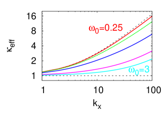
Figure 10: Effective bending stiffness (in units of $N\kappa_{b}$) as a function of shear stiffness $k_{\times}$ (in units of $\kappa_{b}\delta/b^{2}L^{2}$) of a bundle of four filaments under a tip force $F$. The bending stiffness is calculated from the determined end-deflection $y(L)$ by $\kappa_{\rm eff}=FL^{3}/12y(L)$. The full curves are for finite pretwist $\omega_{0}L/\pi=(0.25,0.5,1,2,3)$, while the dashed curves represent the limiting cases of zero and infinite pretwist, repsectively.

VI Conclusions and Outlook

We have presented a detailed study of the elastic and dynamic properties of bundles of semiflexible filaments (wormlike bundle model, WLB). It is found that a competition between the elastic properties of the filaments and those of the crosslinks leads to renormalized effective bend and twist rigidities that can become mode-number dependent. The strength and character of this dependence varies with bundle architecture, such as the arrangement of filaments in the cross section and pretwist.

Two paradigmatic cases of bundle architecture have been discussed (see Fig. 2): the first assumes filaments to be arranged homogeneously throughout the cross-section, for example on a square or triangular lattice. This geometry is particularly relevant for F-actin bundles. The second architecture has the filaments arranged on the surface of a cylinder as is the case for microtubules. For all bundle architectures, the bending rigidity depends on mode-number $q_{n}$ as $\kappa_{B}(n)\sim k_{\times}q_{n}^{-2}$. This is the shear dominated regime, as the bending rigidity is proportional to the shear stiffness, $k_{\times}$, of the crosslinks Bathe et al. (2008). It is in this parameter regime that the bundle behaves qualitatively different than either a homogeneous beam (obtained in the ”fully coupled” limit) or an assembly of ”decoupled” filaments. Each architecture has its own universal ratio of maximal to minimal bending rigidity, independent of the specific type of crosslink induced filament coupling. For microtubules (without pretwist) we find the ratio $r=1+2/\sin^{2}(\pi/N)$, which is in reasonable agreement with the available experimental data.

An important factor in determining the strength of crosslink-induced filament coupling is the pretwist (helicity) of the bundle. Numerical computation shows that the effective bending rigidity decreases with increasing the pretwist. This has interesting consequences for microtubules, where the amount of pretwist depends on the number of protofilaments, $N$. Different microtubule types are therefore predicted to have different variations in their effective bending rigidity. These predictions could be tested in experiments that are able to select the microtubule type and measure their bending rigidity independently.

We have discussed several further observables, static and dynamic, that could be relevant to experiments. We have shown that the concept of the persistence length becomes ambiguous and depends on the observable used. The usual definition via the tangent-tangent correlation function is shown to lead to a persistence-length that depends on the scale of observation. Further observables that are effected by the mode-dependent bending rigidity are the force-extension relation or the buckling force Heussinger et al. (2007). Interestingly, in the intermediate regime the latter is constant and independent of bundle length.

The dynamic properties of bundles are characterized by a complex cross-over scenario which is in one-to-one correspondence with the three regimes of decoupled, intermediate and fully-coupled bending. While decoupled and fully-coupled bending display the usual $t^{3/4}$ in the correlation function, it is shown that the shear-coupling leads to an intermediate asymptotic regime, where the correlations only grow as $t^{1/2}$. The response functions for longitudinal and transverse forces also reflect these different regimes. In contrast to the WLC, they are not just proportional to each other but show distinct frequency dependences. These findings may be relevant for microrheological experiments, with imbedded bead particles directly coupling to the transverse bundle fluctuations.

Possibilities for future studies may be to look into the effects of filament fracture or lattice defects. The elastic energy represents a harmonic approximation which should be extended to include nonlinear effects. Especially for microtubules one may expected nonlinear effects to play an important role in bundle mechanics. For example, it may be important to consider that protofilaments in their unstressed state are not straight but bend radially outwards. Aditional complications could also arise from the fact that some microtubules are not transversly isotropic as we have assumed here, but have a ”seam”, where protofilaments are offset relative to their neighbors. Failure modes under axial compressive forces have been discussed in a model for microtubules that starts from a transversly isotropic shell theory Wang et al. (2006). It would be interesting to compare the results of a generalized WLB model – to include cross-sectional deformations – with their results for the critical buckling forces. One mode of failure, the ovalization of the microtubule cross-section (Brazier effect) may for example be taken into account by adjusting the cross-sectional coordinates with the help of an “ovalization parameter”. This would then have to be determined together with the other degrees of freedom from the equilibrium equations.

Appendix A Exact Solution for bending and twist rigidities

In this appendix the effective bending and twist rigidities are calculated exactly from the WLB Hamiltonian, Eqs. (1) - (II.1). To this end the $u$-variables have to be integrated over to define an effective WLC Hamiltonian.

First, we have to show that there are no terms in the shear Hamiltonian, Eq. (3), that would couple the different Euler angles $\theta,\phi,\psi$. To this end we use Eq. (II.1) in Eq. (3) and specialize to a square cross-section. The resulting shear Hamiltonian can then be written as

$$H_{\rm shear} = \frac{k_{\times}}{2\delta}\int_{s}\sum_{ij}\left[\left(u_{ij}-u_{i+1,j}-b\psi^{\prime}z_{j}+b\phi\right)^{2}\right.$$ (28)

$$+ \left.\left(u_{ij}-u_{i,j+1}+b\psi^{\prime}y_{i}-b\theta\right)^{2}\right]\,,$$

where $y_{i}=b\cdot(i+\frac{1}{2})$ and $z_{j}=b\cdot(j+\frac{1}{2})$. Here, each filament is labeled by the pair of indices $(i,j)$, which denotes its location in the $i$th row and the $j$th column of the square cross-section. The only terms that couple the different Euler angles are $b^{2}\psi^{\prime}\phi\sum_{ij}z_{j}$ and $b^{2}\psi^{\prime}\theta\sum_{ij}y_{i}$. These identically vanish because of the symmetric arrangement of the filaments, $\sum_{j}z_{j}=0$ and $\sum_{i}y_{i}=0$.

The remaining calculations are performed in Fourier-space. For the transformation we use $\cos$-modes, which are appropriate for bundles with pinned boundary conditions. Writing the $u$-dependent part of the Hamiltonian in matrix form $\beta H=\frac{1}{2}\sum_{kl}u_{k}A_{kl}u_{l}+\sum_{l}u_{l}b_{l}$ one needs the following formula valid for a Gaussian integral

$$\int\prod_{k}du_{k}\exp\left(-\frac{1}{2}\sum_{kl}u_{k}A_{kl}u_{l}-\sum_{l}u_{l}b_{l}\right)$$ (29)

$$=\exp\left(-\frac{1}{2}\sum_{kl}\bar{u}_{k}A_{kl}\bar{u}_{l}-\sum_{l}\bar{u}_{l}b_{l}\right)\,,$$

where $\bar{u}$ is obtained from

$$\partial(\beta H)/\partial u_{k}=0\,.$$ (30)

Having found the solution $\bar{u}$, we can finally bring Eq. (29) in the form of Eq. (8) to read off the effective bend and twist rigidities.

A.1 Bending

Here we solve Eq. (30) for the case of bending of the square bundle. It proves useful to introduce the dimensionless crosslink shear stiffness $\alpha=k_{\times}L^{2}/k_{s}\delta^{2}$. We can then write Eq. (30) as

$$(qL)^{2}u_{k}-\alpha\partial^{2}u_{k}=0\,.$$ (31)

We also defined the discrete second derivative $\partial^{2}u_{k}=u_{k+1}-2u_{k}+u_{k-1}$. Note, that we are working in Fourier-space so all quantities should carry an additional subscript relating to the mode-number $n$. As different modes don’t mix, there is no harm in dropping it for the moment.

At the outer edges of the bundle $k=-M,M-1$ we find

$$u_{M-1}-u_{M-2}=\frac{(qL)^{2}}{\alpha}u_{M-2}+b\,\theta\,,$$ (32)

and

$$u_{-M+1}-u_{-M}=\frac{(qL)^{2}}{\alpha}u_{-M}+b\,\theta\,.$$ (33)

The Eq. (31) is solved by $u_{k}=Am_{+}^{k}+Bm_{-}^{k}$, where $m_{\pm}=\frac{1}{2}\left(x\pm\sqrt{x^{2}-4}\right)$ and we have defined $x=2+(qL)^{2}/\alpha$. The constants $A,B$ are adjusted to fulfil the boundary conditions Eqs. (32) and (33). This solution for the axial stretching variable $u_{k}$ is plotted in Fig. 6.

To obtain the approximated bending rigidity of Eq. (10) one first has to insert the assumption $u_{k}=\Delta u\cdot(k+1/2)$ into the Hamiltonian and then minimize with respect to the single variable $\Delta u$.

This way one finds

$$\Delta u=\frac{-b\,\theta}{1+\frac{\sqrt{M}}{6\alpha}(\sqrt{M}+1)}\,,$$ (34)

which has to be reinserted into the Hamiltonian to yield Eq. (10).

A.2 Twist

In the case of pure twisting the same analysis can be done to calculate the effective twist rigidity. The difference to the bending case is that now the full 2d boundary value problem has to be solved. The equation determining the axial stretching $u_{ij}$ of the filament indexed by $(i,j)$ is

$$(qL)^{2}u_{ij}-\alpha\Delta u_{ij}=0,$$ (35)

where the operator $\Delta=\partial^{2}_{i}+\partial^{2}_{j}$ is the two-dimensional version of the discrete Laplacian encountered above. The finite difference operator $\partial_{i}$ is defined as $\partial^{2}_{i}u_{ij}=u_{i+1j}+u_{i-1j}-2u_{ij}$. As for the case of pure bending, here, the twist variable $\psi$ enters only via the boundary terms.

The classic theory to calculate the twist rigidity of beams has been given by Saint-Venant Love (1944). In this approach the axial displacements are found by solving Laplace’s equation $\Delta u(y,z)=0$ on the appropriate domain of the cross-section. We see that Eq. (35) reduces to the Laplace equation in the limit $\alpha\sim k_{\times}\to\infty$, which is the reason why in Fig. 9 the continuum limit is approached with increasing shear stiffness at fixed bundle size. The remaining difference stemming from the discretization into $N$ filaments represents only a small effect. In Saint-Venant theory it is well known that for rectangular domains two types of solutions appear, depending on the aspect-ratio of the cross-section. We illustrate the different symmetry properties of these solutions in Fig. 11.

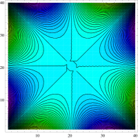
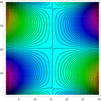
Figure 11: Illustration of the two types of solution obtained for the stretching $u_{ij}$ of filament $(i,j)$. Left: square cross-section of $40\star 40$ filaments. Right: $30\star 40$ filaments

Appendix B Relation between the $\Omega_{\alpha,k}$ of filament $k$ and the $\Omega_{\alpha}$ of the central line

This appendix gives some details on the description of the bundle kinematic degrees of freedom. The goal is to relate the generalized curvatures $\Omega_{\alpha,k}$ of filament $k$, to the $\Omega_{\alpha}$ of the bundle central line. That these need not necessarily coincide is best illustrated by discussing an example. If the central line is twisted but not bent, $\Omega_{3}$ remains as the only non-vanishing component of the curvature vector. The filaments themselves, however, twist and bend as they trace out a helical path with radius $R$. Their bending energy is $\kappa_{f}L(R\Omega_{3}^{2})^{2}$, of fourth order in $\Omega_{3}$.

As a second example consider the bending of the central line, $\Omega_{1}=1/R$, where $R$ is the radius of curvature. The filaments that lie at a distance $b$ away from the central line naturally have a different radius of curvature, $R\pm b$, and thus a different bending energy. The correction is again of higher order and scales as $b^{2}\Omega_{1}^{4}$. It turns out, that all effects like the two just mentioned only contribute to higher order. To lowest order we will find that $\Omega_{\alpha}=\Omega_{\alpha,k}$.

We define the vector $\mathbf{r}_{k}(s)=\mathbf{r}_{0}(s)+\mathbf{R}_{k}(s)$ to point to filament $k$ at arclength position $s$. The central line of the bundle is thereby given by $\mathbf{r}_{0}(s)$. The position of each filament in the cross-section is parametrized by $\mathbf{R}_{k}(s)=A_{k}\mathbf{d}_{1}(s)+B_{k}\mathbf{d}_{2}(s)$, where $A_{k}$ and $B_{k}$ are constants independent of arclength $s$ and deformation of the bundle. This, in particular, implies that in the reference state the filaments are always straight and untwisted. We also need the derivative of $\mathbf{R}_{k}$ with respect to $s$,

$$\mathbf{R}_{k}^{\prime}=(B_{k}\Omega_{1}-A_{k}\Omega_{2})\mathbf{t}+\Omega_{3}\mathbf{R}_{k}^{\perp}$$ (36)

where we have used the Frenet-Seret equations and defined $\mathbf{R}_{k}^{\perp}=B_{k}\mathbf{d}_{1}(s)-A_{k}\mathbf{d}_{2}(s)$. With this the tangent to filament $k$ is given by

$$\mathbf{t_{k}}=\frac{1}{N}((1+B_{k}\Omega_{1}-A_{k}\Omega_{2})\mathbf{t}+\Omega_{3}\mathbf{R}_{k}^{\perp})\,,$$ (37)

with an appropriate normalization factor, $N$. One finds, that the filament tangent is parallel to the central-line only if the twist vanishes, $\Omega_{3}=0$. For finite bundle twist, the filament tangent is rotated around the vector $\mathbf{R}_{k}$ relative to the central tangent $\mathbf{t}$. The magnitude of the rotation is $\Omega_{3}R_{k}$ and depends on the distance $R_{k}=|\mathbf{R}_{k}|=|\mathbf{R}_{k}^{\perp}|$ of the filament to the central line.

In order to derive expressions for the remaining two unit vectors $\mathbf{d}_{1,k}$ and $\mathbf{d}_{2,k}$ let us assume, for the time being, that no other rotation is allowed that may re-orient the local frame of filament $k$ relative to the central frame. With this assumption filaments are not allowed to twist relative to their neighbors as this would correspond to a rotation around $\mathbf{t}_{k}$. In the bundles we consider, this internal twist motion can safely be neglected as crosslinks provide for permanent rigid inter-filament connections. As explained below, these internal twist modes may nevertheless be important at the time of bundle formation.

The local frame can then be related to the central frame by

$$\mathbf{d}_{1,k} = \mathbf{d}_{1}-B_{k}\Omega_{3}\sin\alpha\mathbf{t}+O(b_{k}\Omega_{3})^{2}$$ (38)

$$\mathbf{d}_{2,k} = \mathbf{d}_{2}+A_{k}\Omega_{3}\cos\alpha\mathbf{t}+O(b_{k}\Omega_{3})^{2}$$ (39)

One can now express the generalized curvatures of the filaments in terms of the $\Omega_{\alpha}$ of the central line. For simplicity we here consider the case of pure twisting where $\Omega_{1}=\Omega_{2}=0$. One then finds

$$\Omega_{3,k} \equiv (\partial_{s_{k}}\mathbf{d}_{1,k})\cdot\mathbf{d}_{2,k}$$

$$= \Omega_{3}-\Omega_{3}\Omega_{3}^{\prime}A_{k}B_{k}=\Omega_{3}(1+O(\frac{b^{2}\Omega_{3}}{L}))$$

Note, that the difference in length between the central line and the individual filaments should be taken into account in the parametrization in terms of arclength, however, only contributes to higher orders. More formally, $\partial s/\partial s_{k}=1+O(b\Omega)$.

In addition to twist, filaments also bend

$$\Omega_{1,k} \equiv (\partial_{s_{k}}\mathbf{d}_{2,k})\cdot\mathbf{d}_{3,k}$$ (41)

$$= \Omega_{3}^{\prime}A_{k}+\Omega_{3}^{2}B_{k}$$ (42)

and

$$\Omega_{2,k} \equiv (\partial_{s_{k}}\mathbf{d}_{1,k})\cdot\mathbf{d}_{3,k}$$ (43)

$$= -\Omega_{3}^{\prime}B_{k}+\Omega_{3}^{2}A_{k}\,.$$ (44)

which reduces to the well known expression for the curvature of a helix if $\Omega_{3}^{\prime}=0$.

Finally, let us comment on what would happen if we did allow the filaments to twist individually, and relative to their neighbors. This filament twist can be described by an additional rotation, $\psi_{k}(s)$ of the local unit vectors, $\mathbf{d}_{1,k},\mathbf{d}_{2,k}$ around the tangent $\mathbf{t}_{k}$.

The new vectors are then given by

$$\mathbf{e}_{1,k} = \cos\psi_{k}\mathbf{d}_{1,k}+\sin\psi_{k}\mathbf{d}_{2,k}$$ (45)

$$\mathbf{e}_{2,k} = -\sin\psi_{k}\mathbf{d}_{1,k}+\cos\psi_{k}\mathbf{d}_{2,k}\,,$$ (46)

and the bundle twist, $\Omega_{3}$, can be calculated as before

$$\Omega_{3,k}=\Omega_{3}+\psi_{k}^{\prime}\,.$$ (47)

The twist energy should thus be written as

$$H_{\rm twist} = \frac{\kappa_{t}}{2}\int_{s}\sum_{k}(\Omega_{3}+\psi_{k}^{\prime})^{2}$$

$$= \frac{N\kappa_{t}}{2}\int_{s}(\Omega_{3}+\bar{\psi^{\prime}})^{2}+N(\bar{\psi^{\prime 2}}-{\bar{\psi^{\prime}}}^{2})\,,$$

where we defined the moments of the filament twist distribution $\bar{\psi^{\prime r}}=\sum_{k}{\psi_{k}^{\prime}}^{r}/N$.

As explained above, in crosslinked bundles this internal twist can be assumed to be quenched at the time of bundle formation. In this case we need not treat the $\psi_{k}$ as dynamical variables for the discussion of bundle deformation. A finite $\bar{\psi^{\prime}}$ nevertheless gives the bundle a certain helicity and imposes pretwist, as discussed in Section V.

Appendix C Derivation of shear deformation

To calculate the geometric part $\Delta$ of the shear deformation, an expression for the arclength mismatch between the two points on the filament pair is needed. The general expression is

$$\Delta_{lk}=\Delta s+\int^{s}|\mathbf{t}+\mathbf{R}_{l}^{\prime}|-\int^{s}|\mathbf{t}+\mathbf{R}_{k}^{\prime}|\,,$$ (49)

where the first contribution, $\Delta s$, derives from the possibility that the two points do not correspond to the same point, $s$, on the bundle central line.

By using Eqs. (36), (37) and expanding one finds

$$\Delta=\Delta s+\int_{0}^{s}\left[\mathbf{b}_{lk}^{\prime}\cdot\mathbf{t}-\frac{1}{2}(\mathbf{R}_{l}^{\prime 2}-\mathbf{R}_{k}^{\prime 2})\right]\,,$$ (50)

where, we defined $\mathbf{b}_{lk}=\mathbf{R}_{l}-\mathbf{R}_{k}$ pointing from filament $k$ to filament $l$. As in the formulation of $H_{0}$, only the leading order terms have been accounted for. The $(\mathbf{b}_{lk}^{\prime}\cdot\mathbf{t})$-term only contains bending deformations. This may be seen by setting $\mathbf{t}=\mathbf{\hat{e}}_{x}=\rm{const}$ appropriate for a pure twisting of the central line. Then $\Delta_{lk}=\mathbf{b}_{lk}\cdot\mathbf{\hat{e}}_{x}=0$ as the vector $\mathbf{b}_{lk}$ lies within the cross-section, that is perpendicular to the tangent.

The last term corresponds to the arclength-difference acquired between two filaments at different distance to the central-line ($R_{k}\neq R_{l}$). It is clear that the filament farther out has to go a longer distance, so its crosslinking sites will stay back in comparison to that of its neighbor closer in the center of the bundle. However, twist also produces shear deformation between filaments which lie at equal distance to the central line ($R_{l}=R_{k}$). This is embodied in the extra term $\Delta s$, which we treat now (also see Fig. 4). To derive an expression for the shear displacement in this case, assume that the two filaments lie, separated by a distance $b_{lk}=|\mathbf{b}_{lk}|$, on the surface of a cylinder of radius $R$. Twisting the cylinder makes the filaments wind around it, each taking an angle $\Omega_{3}R$ to the cylinder axis. The shear deformation then simply is $\Delta s=\Omega_{3}Rb_{lk}$. For arbitrary orientation of the filament pair we have to write $\Delta s=\mathbf{t}_{lk}\cdot\mathbf{b}_{lk}$, where $\mathbf{t}_{lk}$ is the tangent to the midline between the filament pair. In agreement to what has been said above, this mechanism does not contribute to the shear displacement when the filament pair $(l,k)$ is connected by crosslinks in radial direction. In this case, $\mathbf{t}_{lk}\perp\mathbf{b}_{lk}$, and the shear deformation $\Delta s=0$.

References

- Mogilner and Rubinstein (2005) A. Mogilner and B. Rubinstein, Biophys. J. 89, 782 (2005).
- Atilgan et al. (2006) E. Atilgan, D. Wirtz, and S. X. Sun, Biophys. J. 90, 65 (2006).
- Vignejvic et al. (2006) D. Vignejvic, S. Kojima, Y. Aratyn, O. Danciu, T. Svitkina, and G. G. Borisy, J. Cell Biol. 90, 65 (2006).
- Hudspeth and Corey (1977) A. J. Hudspeth and D. P. Corey, Proc. Natl. Acad. Sci. USA 74, 2407 (1977).
- Schmid et al. (2004) M. F. Schmid, M. B. Sherman, P. Matsudaira, and W. Chiu, Nature 431, 104 (2004).
- Howard (2008) J. Howard, Cellular and Molecular Bioengineering 1, 24 (2008).
- Claessens et al. (2006) M. M. A. E. Claessens, M. Bathe, E. Frey, and A. R. Bausch, Nature Mat. 5, 748 (2006).
- Pelletier et al. (2003) O. Pelletier, E. Pokidysheva, L. S. Hirst, N. Bouxsein, Y. Li, and C. R. Safinya, Phys. Rev. Lett. 91, 148102 (2003).
- Lieleg et al. (2007) O. Lieleg, M. Claessens, C. Heussinger, E. Frey, and A. R. Bausch, Phys. Rev. Lett. 99, 088102 (2007).
- Schmoller et al. (2008) K. M. Schmoller, O. Lieleg, and A. R. Bausch, Phys. Rev. Lett. 101, 118102 (2008).
- Bathe et al. (2008) M. Bathe, C. Heussinger, M. M. A. E. Claessens, A. R. Bausch, and E. Frey, Biopys. J. 94, 2955 (2008).
- Heussinger et al. (2007) C. Heussinger, M. Bathe, and E. Frey, Phys. Rev. Lett. 99, 048101 (2007).
- Kratky and Porod (1949) O. Kratky and G. Porod, Rec. Trav. Chim. Pays-Bas. 68, 1106 (1949).
- Saitô et al. (1967) N. Saitô, K. Takahashi, and Y. Yunoki, J. Phys. Soc. J. 22, 219 (1967).
- Gov (2008) N. S. Gov, Phys. Rev. E 78, 011916 (2008).
- Guild et al. (2003) G. M. Guild, P. S. Connelly, L. Ruggiero, K. A. Vranich, and L. G. Tilney, J. Cell Biol. 162, 1069 (2003).
- Claessens et al. (2008) M. M. A. E. Claessens, C. Semmrich, L. Ramos, and A. R. Bausch, Proc. Natl. Acad. Sci. USA 105, 8819 (2008).
- Purdy et al. (2007) K. R. Purdy, J. R. Bartles, and G. C. L. Wong, Phys. Rev. Lett. 98, 058105 (2007).
- Hilfinger and Jülicher (2008) A. Hilfinger and F. Jülicher, Phys. Biol. 5, 016003 (2008).
- Alim and Frey (2007) K. Alim and E. Frey, Eur. Phys. J. E 24, 185 (2007).
- Goldstein et al. (2002) H. Goldstein, C. Poole, and J. Safko, Classical Mechanics (Addison Wesley, San Francisco, 2002), 3rd ed.
- Everaers et al. (1995) R. Everaers, R. Bundschuh, and K. Kremer, Europhys. Lett. 29, 263 (1995).
- Mergell et al. (2002) B. Mergell, M. R. Ejtehadi, and R. Everaers, Phys. Rev. E 66, 011903 (2002).
- Golestanian and Liverpool (2000) R. Golestanian and T. B. Liverpool, Phys. Rev. E 62, 5488 (2000).
- Zhou et al. (2000) H. Zhou, Y. Zhang, and Z. can Ou-Yang, Phys. Rev. E 62, 1045 (2000).
- Mohrbach and Kulic (2007) H. Mohrbach and I. M. Kulic, Phys. Rev. Lett. 99, 218102 (2007).
- Love (1944) A. E. H. Love, The Mathematical Theory of Elasticity (Dover, New York, 1944), 4th ed.
- Calladine (1983) C. R. Calladine, Theory of shell structures (Cambridge University Press, 1983).
- Landau and Lifschitz (1970) L. D. Landau and E. M. Lifschitz, Theory of Elasticity (Pergamon Press, Oxford, 1970).
- Gere and Timoshenko (2002) J. M. Gere and S. P. Timoshenko, Mechanics of Materials (Nelson Thornes Ltd, Cheltenham, 2002), 5th ed.
- Kis et al. (2002) A. Kis, S. Kasas, B. Babić, A. J. Kulk, W. Benoît, G. A. D. Briggs, C. Schönenberger, S. Catsicas, and L. Forró, Phys. Rev. Lett. 89, 248101 (2002).
- Pampaloni et al. (2006) F. Pampaloni, G. Lattanzi, A. Jonás, T. Surrey, E. Frey, and E.-L. Florin, Proc. Natl. Acad. Sci. USA 103, 10248 (2006).
- Kis et al. (2004) A. Kis, G. Csányi, J.-P. Salvetat, T.-N. Lee, E. Couteau, A. J. Kulik, W. Benoit, J. Brugger, and L. Forró, Nature Mat. 3, 153 (2004).
- Nelson and Peliti (1987) D. Nelson and L. Peliti, J. Physique 48, 1085 (1987).
- Nelson et al. (2004) D. Nelson, T. Piran, and S. Weinberg, eds., Statistical Mechanics of Membranes and Surfaces (World Scientific, 2004), 2nd ed.
- Frey and Nelson (1991) E. Frey and D. R. Nelson, J. Phys. 1 1, 1715 (1991).
- Kroy and Frey (1997) K. Kroy and E. Frey, Phys. Rev. E 55, 3092 (1997).
- Isambert and Maggs (1996) H. Isambert and A. C. Maggs, Macromolecules 29, 1036 (1996).
- Gittes and MacKintosh (1998) F. Gittes and F. C. MacKintosh, Phys. Rev. E 58, R1241 (1998).
- Morse (1998a) D. C. Morse, Phys. Rev. E 58, R1237 (1998a).
- Morse (1998b) D. C. Morse, Macromolecules 31, 7044 (1998b).
- Koenderink et al. (2006) G. H. Koenderink, M. Atakhorrami, F. C. MacKintosh, and C. F. Schmidt, Phys. Rev. Lett. 96, 138307 (2006).
- Granek (1997) R. Granek, J. Physique II 7, 1761 (1997).
- Frey et al. (2000) E. Frey, K. Kroy, and J. Wilhelm, The Wiley Polymer Networks Group Review (John Wiley, 2000), vol. 2.
- Kroy and Glaser (2007) K. Kroy and J. Glaser, New J. Phys. 9, 416 (2007).
- Chrétien et al. (1992) D. Chrétien, F. Metoz, F. Verde, E. Karsenti, and R. H. Wade, J. Cell Bio. 117, 1031 (1992).
- Chrétien and Wade (1991) D. Chrétien and R. H. Wade, Biol. Cell 107, 161 (1991).
- Kurachi et al. (1995) M. Kurachi, M. Hoshi, and H. Tashiro, Cell Motil. Cytoskeleton 30, 221 (1995).
- Kikumoto et al. (2006) M. Kikumoto, M. Kurachi, V. Tosa, and H. Tashiro, Biophys. J 90, 1687 (2006).
- Brangwynne et al. (2007) C. P. Brangwynne, G. Koenderink, E. Barry, Z. Dogic, F. C. MacKintosh, and D. A. Weitz, Biophys. J. 93, 346 (2007).
- Taute et al. (2008) K. M. Taute, F. Pampaloni, E. Frey, and E.-L. Florin, Phys. Rev. Lett. 100, 028102 (2008).
- van den Heuvel et al. (2008) M. G. L. van den Heuvel, M. P. de Graaff, and C. Dekker, Proc. Nat. Acad. Sci. USA 105, 7941 (2008).
- van den Heuvel et al. (2007) M. G. L. van den Heuvel, S. Bolhuis, and C. Dekker, NanoLett. 7, 3138 (2007).
- Janson and Dogterom (2004) M. E. Janson and M. Dogterom, Biophys. J. 87, 2723 (2004).
- Gittes et al. (1994) F. Gittes, B. Mickey, J. Nettleton, and J. Howard, J Cell Biol 120, 923 (1994).
- Grason and Bruinsma (2007) G. Grason and R. Bruinsma, Phys. Rev. Lett. 99, 098101 (2007).
- Grason (2009) G. M. Grason, Phys. Rev. E 79, 041919 (2009).
- Wang et al. (2006) C. Y. Wang, C. Q. Ru, and A. Mioduchowski, Phys. Rev. E 74, 052901 (2006).
- Ferrer et al. (2008) J. M. Ferrer, H. Lee, J. Chen, B. Pelz, F. Nakamura, R. D. Kamm, and M. J. Lang, Proc. Natl. Acad. Sci. USA 105, 9221 (2008).
- Lee et al. (2009) H. Lee, B. Pelz, J. Ferrer, T. Kim, M. Lang, and R. Kamm, Cellular and Molecular Bioengineering 2 (2009).
- Miyata et al. (1996) H. Miyata, R. Yasuda, and K. Kinosita, Biochim Biophys Acta 1290, 83 (1996).