Interferometric observations of the hierarchical triple system Algol

Abstract

Algol is a triple stellar system consisting of a close semi-detached binary orbited by a third object. Due to the disputed spatial orientation of the close pair, the third body perturbation of this pair is the subject of much research. In this study, we determine the spatial orientation of the close pair orbital plane using the CHARA Array, a six-element optical/IR interferometer located on Mount Wilson, and state-of-the-art e-EVN interferometric techniques. We find the longitude of the line of nodes for the close pair is $\Omega_{1}=48\arcdeg\pm 2\arcdeg$ and the mutual inclination of the orbital planes of the close and the wide pairs is $95\arcdeg\pm 3\arcdeg$. This latter value differs by $5\arcdeg$ from the formerly known $100\arcdeg$ which would imply a very fast inclination variation of the system, not borne out by the photometric observations. We also investigated the dynamics of the system with numerical integration of the equations of motions using our result as an initial condition. We found large variations in the inclination of the close pair (its amplitude $\sim 170\arcdeg$) with a period of about 20 millenia. This result is in good agreement with the photometrically observed change of amplitude in Algol’s primary minimum.

1 Introduction

There are about 1000 triple stellar systems known in the Galaxy, many of which consist of a close eclipsing pair and a distant third object orbiting around the close pair (Batten 1973, Tokovinin 1997). Algol is probably the most well-known of such systems.

Algol consists of a semi-detached eclipsing binary with an orbital period of 2.87 days (B8V + K2IV) with an F1IV spectral type star revolving around the binary every 680 days (discovered by radial velocity measurements, Curtiss 1908). Early interferometric observations were unable to resolve the system (Merrill 1922), but the third component was succesfully observed by speckle interferometry (Gezari, Labeyrie and Stachnik 1972, Blazit et al. 1977, McAlister 1977, 1979) and its orbit was precisely determined by Bonneau (1979). This result was refined by using the Mark III optical stellar interferometer (Pan et al. 1993).

In the radio regime, Lestrade et al. (1993) detected positional displacement during the orbital revolution of the AB pair using the VLBI technique, and identified the K-subgiant as the source of radio emission. The orbital elements of the close and the wide pairs determined from all these observations are listed in Table 1.

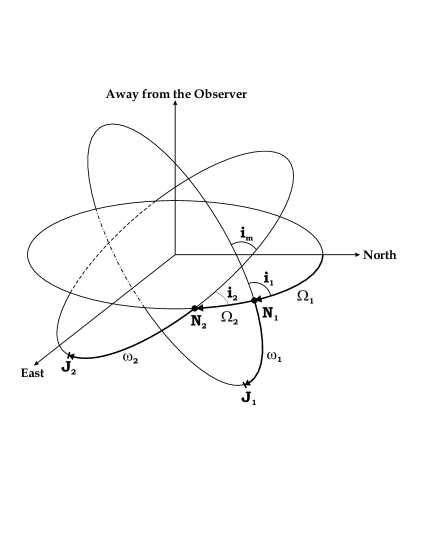
Figure 1: The meaning of different angular orbital elements mentioned in this paper. Orbits are projected into a sphere. $\Omega_{1}$, $\Omega_{2}$ are the longitudes of the nodes of the close and the wide pair, respectively, $N_{1}$, $N_{2}$ are the ascending nodes. $i_{1}$ and $i_{2}$ denotes the inclinations of the orbits measurable by an observer while $i_{m}$ is the mutual inclination of the two orbital planes. $J_{1}$ and $J_{2}$ are the pericentre points.

The light minima – mainly primary – of Algol were extensively observed in the last two centuries. There was only a very small change in the eclipse depth during this time. This led Söderhjelm (1975, 1980) to the theoretical conclusion that the mutual inclination of the orbital planes of the close and the wide pair systems should not be larger than $11\arcdeg$ and likely they are coplanar because both the shape and depth of the light minima should have noticeably changed otherwise. This theoretical result was seemingly in good correspondence with the inclination data deduced both for the close and the wide orbits, i.e. $i_{1}=82\fdg 3\pm 0\fdg 2$, and $i_{2}=83\arcdeg\pm 2\arcdeg$ (Söderhjelm 1980) (see also Figure  1), respectively, from which Söderhjelm (1980) stated the exact coplanarity. Based on the earliest speckle interferometric measurements, Söderhjelm (1980) calculated $\Omega_{2}=132\arcdeg\pm 2\arcdeg$ for the wide orbit, and therefore he expected $\Omega_{1}=132\arcdeg\pm 4\arcdeg$ for the node of the eclipsing pair. Later Pan et al. (1993) determined the astrometric orbit of the third component and found that both the longitude of the ascending node ($\Omega_{2}$) and the argument of the periastron ($\omega_{2}$) of the wide orbit practically differ by $180\arcdeg$ from the previously accepted values. In the case of an isolated two-body astrometric orbit, $180\arcdeg$ discrepancy is non-problematic, because geometrically it means the reflection of the orbital plane onto the plane of the sky for which transformation the astrometric coordinates are invariants. Nevertheless, in a triple body system this results in different spatial configuration of the orbital planes, i.e. it modifies the mutual inclination fundamentally. However, the polarimetric measurements of Rudy (1979) yielded a contradictory result, suggesting that $\Omega_{1}=47\arcdeg\pm 7\arcdeg$ which would imply a perpendicular rather than coplanar configuration. Nevertheless, Söderhjelm (1980) suggested, that perhaps the nature of the polarization mechanism was not understood correctly. Note that Rudy (1979) resolved also the inclination ambiguity, i.e. he determined that the angular momentum of the binary directed away from the observer, and, consequently, the system inclination ($i_{1}$) should be less than $90\arcdeg$.

This nearly perpendicular configuration was supported by other measurements: Lestrade et al. (1993) found $\Omega_{1}=52\arcdeg\pm 5\arcdeg$ for the close pair in good agreement with the polarimetric measurements of Rudy (1979). If this value of $\Omega_{1}$ is correct, then the mutual inclination is about $100\arcdeg$ (Kiseleva et al. 1998), and the two orbital planes are nearly but not exactly perpendicular to each other. This value for the mutual inclination of the system has been widely accepted since then. However, we propose that this mutual inclination value cannot be correct due to dynamical considerations which is described hereafter.

It is well-known that in a hierarchical triple stellar system, the orbital planes of the close and wide pairs are subject to precessional motion, in such a way that the normals of the orbital planes move on a conical surface around the normal of the invariable plane. (Here we omit the effect of stellar rotation which is insignificant in an ordinary triple system.) In the case of a hierachical triple system where the invariable plane almost coincides with the wider orbital plane, the precession cone angle is close to the mutual inclination. Consequently, in the case of the present system, we would get an almost $160\arcdeg$-amplitude variation in the observable inclination during the approximate period given by Eq. (27) of Söderhjelm (1975) (assuming the present approximation is valid, when the mutual inclination tends to $90\arcdeg$, the precession period tends to infinity). Here we refer to Fig. 4 of Borkovits et al. (2004) which clearly shows that in the case of the aforementioned configuration the observable inclination of the close binary would have changed by approximately $3\arcdeg$ in the last century which evidently contradicts the observations. In this case the eclipses would disappear within a few centuries. This was already observed in some eclipsing binaries, like in SS Lacertae or V907 Sco (see e.g. Eggleton & Kiseleva-Eggleton 2001) but not in Algol.

In summary, the polarimetric and the interferometric observations contradict the coplanar-configuration, but – since the mutual inclination is far from exact perpendicularity – the latter is not in agreement with the observed tiny change in the minima depth. A closer approximate perpendicularity of the two orbital planes would mean that the period of orbital precession becomes so large that the inclination variation (and consequently the depth variation of the minimum) of the close pair remains unobservable for a long time, consistent with the observations.

The aim of this study was to constrain the mutual inclination of the system better, requiring the measurement of the longitude of the node for the close pair. The other orbital elements are well-known from spectroscopic or photometric data, but there is a controversy in the value of $\Omega_{1}$. Because the expected apparent size of the close binary semi-major axis is of the order of 2 milliarcseconds (mas), we carried out optical and radio interferometry measurements. As we will show, optical and radio interferometry are complementary techniques. Combining these two, we will show that it is possible to resolve the ambiguity in the geometry of the system, and better assess the accuracy of our measurements.

2 Observations and data reduction

2.1 CHARA Observations

The CHARA Array is an optical/near-IR interferometer array consisting of six 1m telescopes. The array is described in detail in ten Brummelaar et al. (2005). A detailed overview and further references about the observables and the theory of optical interferometry can be found in Haniff (2007).

We observed Algol on three nights (2, 3 and 4 December, 2006) in the $K_{s}$ band (the effective wavelength was $2.133~{}\mu$m). Much of the second night was lost due to high winds and dusty conditions.

Iota Persei and Theta Persei served as calibration stars. The observations of the target and the two calibrators were organized into a sequence and the measurements on calibrators generally bracketed the target observations. We have 12 data points of Iota Persei, 12 data points of Theta Persei and 23 data points of Algol itself.

Each data point was calculated from a number of scans. Each scan measured the intensity variations as a function of the path delay. About 300 scans were collected within five minutes for one data point, the first 22 of these were obtained on the targets (Algol or one of the calibrator stars), then 21 scans were done for measuring the background while the shutter was closed, then more than 200 other scans were obtained on the targets again and finally 67 further scans for measuring the background again.

To reduce the data, we used the recipe of McAlister (2002). This consisted of the following steps: First a low-pass filter was applied to remove the atmospheric noise. Then the bias was subtracted and the scans were normalized to unity. As a next step, the scans measured by the two channels were subtracted from each other (for details, see ten Brummelaar et al. 2005 and McAlister 2002). This was further processed by applying a high-frequency filter to reduce noise. Discrete Fourier-transforms of the scans were calculated and a template was computed. For this new template, we used the full amplitude for the frequencies $\pm 25/$cycle around maximum frequency and 20% of the amplitude for the other frequencies (for more details see McAlister 2002). From this we could calculate the maximum deviation of the template from zero which yielded an estimation of the visibility value. Removing outlier values, we averaged the remaining values which yielded the uncalibrated visibility of a particular point. The error was estimated as the standard deviations of the visibility values of the more than 200 scans of the point.

The measured visibilities of the calibrators were linearly interpolated for the times of the Algol observations. A comparison of the true and measured visibilities of the calibrators yielded a factor which converted the measured target visibilities to true ones. The true visibilities of the two calibrators were estimated as follows:

The uniform disc (UD) angular diameter of Iota Persei is $1.21\pm 0.06$ mas according to the ’Catalog of High Angular Resolution Measurements’ (Richichi et al. 2005). The true diameter of the other calibrator star Theta Persei is $1.201\pm 0.015R_{\odot}$ which was determined by the fit of its spectrum (Valenti and Fisher 2005). Since its HIPPARCOS parallax is known one can easily calculate its true UD angular diameter to be $0.995\pm 0.01$ mas.

The limb-darkened (LD) angular diameter is larger than the UD diameter. There exists a simple relationship between them (Hanbury Brown et al. 1974):

$$\frac{\theta_{\mathrm{LD}}}{\theta_{\mathrm{UD}}}=\sqrt{\frac{1-u_{\lambda}/3}{1-7u_{\lambda}/15}}$$ (1)

The limb-darkening coefficients for both components were taken from the tables of van Hamme (1993). These coefficients are a function of surface gravity and effective temperature which themselves were estimated from the known spectral type of the calibrators. Then Eq. (1) yielded the corrections which increase the UD angular diameters by a few percent only. These corrected values were used to calibrate the visibilities.

The telescope combinations, epoch of observations, baselines, uncalibrated visibilities and their errors can be found in Table 2. The UV-coverage can be seen in Fig. 2

2.2 e-VLBI Observations

We observed Algol with a subset of the European VLBI Network (EVN) between 16:37 and 1:19 UT on 14-15 December 2006 at 5 GHz. These observations were carried out using the e-VLBI technique, where the telescopes stream the data to the central data processor (JIVE, Dwingeloo, the Netherlands) instead of recording. Using e-VLBI for the observations was not fundamental for our measurements, but we took the opportunity of an advertised e-VLBI run close in time to the CHARA observations, outside the normal EVN observing session. The participating telescopes were Cambridge and Jodrell Bank (UK), Medicina (Italy), Onsala (Sweden), Toruń (Poland) and the Westerbork phased array (the Netherlands). The data rate per telescope was 256 Mbps, which resulted in 4$\times$8 MHz subbands in both LCP and RCP polarizations using 2-bit sampling. The correlation averaging time was 2 seconds, and we used 32 delay steps (lags). Initial clock searching was carried out before the experiment using the fringe-finder source 3C345. Algol was phase-referenced (Beasley & Conway 1995) to 0309+411 in 3–5–3 minute cycles. Additional scans were scheduled on 3C84 for real-time fringe monitoring, and for D-term calibration. We used 3C138 to calibrate the Westerbork synthesis array amplitudes and polarization.

Post-processing was done using the US National Radio Astronomy Observatory (NRAO) AIPS package (Diamond 1995). The amplitudes were calibrated using the known antenna gaincurves and the measured system temperatures. The data were fringe-fitted, bandpass calibrated, and then polarization calibrated. We corrected for the polarization leakage D-terms and fringe-fitted the cross-hand data, after which the data were averaged in frequency in each subband. Besides the standard procedure, we used the WSRT synthesis array measurements on 0309+411 to obtain a more accurate VLBI flux scale. The phase-reference source showed a low level of circular polarization (fractional CP $\sim 0.28\%$). The left and right-handed VLBI gains were separately adjusted in accordance with the WSRT measurement. Imaging was carried out in Difmap (Shepherd et al. 1994). The snap-shot images (from about 45 minutes data each) were made by Fourier-transforming the observed visibilities, no self-calibration was applied. We fit circular Gaussian model components to the $uv$-data in Difmap. Initially one component was fit in each snapshot. Then, the size and flux of the component was fixed, and we let the position vary for each 5-minutes Algol scan.

The log of the observations as well as the calculated individual relative positions can be found in Table 3.

3 Data analysis and results

3.1 Analysis of CHARA data

According to the van Cittert-Zernike theorem, the amplitude of the visibility is the normalized Fourier-transform of the intensity distribution (for a comprehensive explanation, see Haniff 2007):

$$V(u,v,t)=\frac{\int\int I(x,y,t)\cos\left(2\pi\frac{u(t)x+v(t)y}{\lambda}\right)\mathrm{d}x\mathrm{d}y}{\int\int I(x,y,t)\mathrm{d}x\mathrm{d}y}$$ (2)

In this equation $V$ is the true visibility at the ($u$, $v$) spatial frequencies, ($x$, $y$) are the corresponding sky coordinates, $t$ is the time, $I$ is the intensity at the ($x,y$) sky point and finally $\lambda=2.133~{}\mu$m is the effective wavelength of our observations (corresponding to the $K_{s}$ band). Note that the intensity distribution on the sky normally changes very slowly with time, but we had to include the time dependence in Eq. (2) because of the rapid orbital revolution of the AB pair. Because of the power of CHARA, it is not enough to model the system as the combination of two point-like sources but we need to combine the pictures of two extended sources.

To determine this intensity distribution we developed a model which was very close to the one of Wilson and Devinney (1971) which is based on the Roche-model (Kopal 1978) but it was implemented in IDL to restore the surface intensities into a matrix and to calculate the sky-projected picture of the system.

Since we have only about two dozen visibility measurements, we wanted to limit the number of free parameters, choosing just three: the angular size of the semi-major axis (in mas), the $K_{s}$ surface brightness ratio, and the angle $\Omega_{1}$. All other parameters were fixed according to the values given in Wilson et al. (1972) or in Kim (1989).

The model outlined above was used to fit the data and a grid search was carried out on the free parameters:

• The surface brigthness ratio was stepped from $0$ to $1.4$ with a step size of 0.05;

• $\Omega_{1}$ was stepped from $0\arcdeg$ to $180\arcdeg$ with a stepsize of $5\arcdeg$ (note that the visibility amplitude does not change if we rotate the image by $180\arcdeg$, which leaves a $180\arcdeg$ ambiguity in the ascending node; this ambiguity in $\Omega_{1}$ can be resolved with VLBI); and

• the angular size of the semi-major axis was stepped from $1.80$ mas to $3.60$ mas with a step-size of 0.005 mas (note that the expected size was $2.50$ mas).

Nearly 353 000 models were calculated on this grid, and the $\chi^{2}$ minimum was found. Around the minimum, a new search was carried out with a finer grid and about 35 000 new models were computed again. Around the minimum, a polynomial fit yielded the final values and errors. The results are shown in Figs. 3 and 4.

The best solution we found is reported in Table 4.

3.2 Analysis of e-VLBI data

The EVN measurements were carried out on 14/15 December 2006 for almost 9 hours. As the orbital period of the eclipsing binary is $P=2.8673$ days, the orbital arc covered was near 13%. During this period a secondary minimum occurred which was simultaneously observed photometrically by the 50-cm telescope at Piszkéstető Station of the Konkoly Observatory, Hungary (see Bíró et al., 2007). One of our goals was to observe possible partial occultation of the radio source by the primary component and measure the change in the circular polarization properties of the source accordingly. Because Algol flared during the observations (see Fig. 5), this goal could not be fulfilled and will not be discussed further here.

In contrast to the measurements of Lestrade et al. (1993) who observed the Algol on four different nights in near quadrature phases (i.e. around $\phi=0.25$ and $\phi=0.75$), our observations covered a small part of the orbit around $\phi\sim 0.5$, when the arc projected onto the plane of the sky is the largest. (Naturally the case is the same at $\phi\sim 0$). The advantage of this approach is that the motion of the target can be detected in a few hours, and the measured positions are only slightly affected by the orbital motion of the AB-C pair, unlike the case when the data are taken at different epochs. Because of the short observing time interval, the orbit of the AB pair itself is not well constrained. Nevertheless, using a priori known values for most of the other orbital parameters, one expects to find a relatively accurate value for the longitude of the ascending node.

There are two limitations that must be mentioned here, 1) short-term tropospheric and ionospheric phase fluctuations which cannot be modelled well and limit the astrometric accuracy in short VLBI-measurements, and 2) the variable structure of the radio source (Mutel et al. 1998) – the radio emission is not coming from the surface of the K-subgiant, but likely from its active polar coronal region. Although Algol was unresolved with our array configuration, the source centroid position could have changed appreciably because of the bright flare during the run. These are the factors that must be taken into account in the interpretation of the final result.

We calculated astrometric orbits as well as a simple linear fit on two different sets of observing data. First, hourly normal points were formed. Then we also calculated the orbit using 5 minutes averages. The latter showed that some points with extremely large scatter can lead to false result in the hourly normal points. Removing such outliers, we calculated our final solution from the 5-minute-average data. Despite the shortness of our observing session (less than 9 hours) the positional data were corrected for the annual parallax, proper motion and the revolution around the centre of mass of the triple system. These corrections resulted in approximately $1\arcdeg$ difference in the node position. For this latter correction we recalculated the third body orbit by the same code which was used for the binary orbit determination from our e-VLBI data. We used both the data sets of Bonneau (1979) and Pan et al. (1993). From these (very similar results) we applied the orbital elements obtained from Pan’s data (see Table 5) for the wide orbit correction. For the astrometric calculations, we used our own differential correction code based on a Levenberg-Marquardt algorithm, tested against the data and results of Eichhorn and Xu (1990), and found it to be in excellent agreement. In our code the maximum number of adjustable free parameters is nine: the position of the centre of mass ($X_{0}$, $Y_{0}$), the orbital period ($P$), and the six usual orbital elements ($a$, $e$, $i$, $\omega$, $\Omega$, and $M_{0}$). In the case of the close binary orbit determination, because of the circular orbit, instead of the argument of periastron ($\omega$), and the mean anomaly ($M$), their sum, i.e., the true longitude (the distance from the ascending node in case of circular orbits) should be used. This was done in such a way, that $\omega_{1}$ was formally considered as zero, while $(M_{0})_{1}=90\arcdeg$ was set for the mid-(secondary) eclipse moment, $t_{0}=2\,454\,084.360$. The period and the inclination were acquired from Kim (1989), while the semi-major axis of the secondary’s orbit around the centre of mass of the binary ($a_{B}$) was calculated from Kim’s data. First we adjusted three parameters ($X_{0}$, $Y_{0}$, $\Omega_{1}$), leaving the other six parameters fixed. Finally, the semi-major axis ($a_{B}$) was also adjusted, as a fourth parameter.

Using Gnuplot, we also performed a simple linear fit to the data from the knowledge that in the vicinity of $\phi=0.5$ the motion can be approximated well with a line whose slope gives $\tan\Omega_{1}$.

Our solutions can be seen in Table 5, as well as in Fig. 6.

4 Discussion

4.1 Discussion of the results

First, we concentrate on the CHARA results. The true size of the semi-major axis of Algol is $a_{1}=14.1~{}R_{\odot}$ (Kim 1989) while its angular size was measured by us to be $a_{1}=2.28\pm 0.02$ mas (see Table 4). By dividing these two numbers one can find that the distance to Algol is $28.6\pm 0.3$ parsec. The HIPPARCOS parallax yielded $28.46^{+0.75}_{-0.71}$ parsec. The agreement is excellent.

The determined surface brightness ratio (0.33) can be converted to a luminosity ratio by multiplying with the ratio of surface area of the two stars, which is known from the light curve solution (Wilson et al. 1972; Kim 1989). The resulting luminosity ratio is 0.43. This value is very close to the photometrically estimated 0.44 (Murad and Budding 1984).

According to the CHARA results, the longitude of the node is $\Omega_{1}=48\arcdeg\pm 2\arcdeg$ with an ambiguity of 180 degrees. Because the determined distance and luminosity ratios agree very well with earlier measurements obtained with other methods, we have confidence in our results. With the VLBI measurements (see below) we resolve the $\pm 180\arcdeg$ ambiguity and conclude that $\Omega_{1}=48\arcdeg\pm 2\arcdeg$. This is in excellent agreement with the value determined from polarimetric measurements ($\Omega_{1}=47\arcdeg\pm 7\arcdeg$, Rudy 1979), indicating that polarimetry is an efficient tool to determine the spatial orientation of the orbits.

At this point we can determine the mutual inclination $i_{m}$ with the following formula:

$$\cos i_{m}=\cos i_{1}\cos i_{2}+\sin i_{1}\sin i_{2}\cos(\Omega_{1}-\Omega_{2})$$ (3)

The result is $i_{m}=95\arcdeg\pm 3\arcdeg$ (the uncertainty reflects the uncertainties not only in $\Omega_{1}$ but also in the other angular elements), confirming the conclusion of Lestrade et al. (1993) that the two orbital planes are nearly perpendicular to each other. This value is, however, closer to the exact perpendicularity than the $100\arcdeg$ given in Kiseleva et al. (1998) which was based on the measurements of Lestrade et al. (1993). Nevertheless, the exact perpendicularity is within the three sigma range.

Regarding the e-VLBI measurements (see Table 5), we obtained $\Omega_{1}=53\arcdeg\pm 826\arcdeg$ and $\Omega_{1}=53\arcdeg\pm 239\arcdeg$ for the node from the three and four adjusted parameter astrometric fits respectively, and $\Omega_{1}=52\arcdeg\pm 3\arcdeg$ from the simple linear LSQ fitting. These values are close to those obtained previously. However, we note that in the case of the astrometric orbit fittings, the formal errors are extremely large. This naturally reflects the fact that our measurements cover only a very short fraction of the orbit, and especially in that phase, where the expected astrometric orbit is almost a straight line. Consequently, without any a priori information, the orbit would be completely undeterminable. However, in this particular case, the longitude of the node itself is very well determined during this phase, as this is nothing other than the slope of the obtained straight line. This is well represented by our linear fit which gives only a minor formal error. So, we think that despite the large formal errors of the astrometric fittings, the obtained $\Omega_{1}$ value, at least for the case in hand should be correct.

We have to remark that the displacement of the radio source during our observing session was almost twice the value which was expected from the pure orbital motion. Formally, of course, we were able to fit an astrometric orbit with a semi-major axis of $a_{B}=0\farcs 0035$, but the semi-major axis of the secondary’s absolute orbit should be $a_{B}=0\farcs 0019$. Nevertheless, although our four-adjustable-parameter fit gave an unreastically large value for the semi-major axis, and consequently, should be rejected, it gave the same value for $\Omega_{1}$ as the three-parameter (fixed $a_{B}$) fit. This also suggests, that despite the large formal errors, the value obtained for $\Omega_{1}$ seems to be well-determined. This apparent large displacement or scatter is likely the consequence of the positional errors caused by short-term atmospheric phase fluctuations, and the variable structure of the source during the flare. This would not be unprecedented. Large positional change was observed in the RS CVn system IM Peg during a flare by Lebach et al. (1999). These structural variations and the origin of large radio flares in Algol could be studied with VLBI array configurations and observing frequencies providing (sub-)mas angular resolution.

4.2 Comparison to former VLBI measurements

Before further discussion of the dynamical consequence of our result, we feel it necessary to comment on the well-known VLBI result of Lestrade et al. (1993). In our opinion it is without question that the excellent paper of Lestrade et al. (1993) is epoch-making in its significance, but, unfortunately, at the last step of their analysis they made some mistakes. As we cited earlier they obtained $\Omega_{1}=52\arcdeg$. A careful look at their Fig. 3 clearly shows that this cannot be the correct result. One can see in that figure, that the coordinate difference is larger in the declination direction than in the right ascension one. Consequently, the slope of the straight line fitted to their four points should be less than $45\arcdeg$, at least, when it is measured from north to east (i.e. from $\delta$ to $\alpha$). So, in our opinion, they obtained their value by measuring from east to north, and so their correct result should be $\Omega_{1}=38\arcdeg\pm 5\arcdeg$. Furthermore, we found, that the exchange of the ($\delta$, $\alpha$) coordinate pairs was not limited only to the determination of $\Omega_{1}$, but it was applied in their all astrometric calculations. A less critical further consequence is that they obtained a reversed orbital revolution (compare their Fig. 4 with our Fig. 7). However, the case of the correction for the orbital motion in the triple system is more problematic. Due to the aforementioned exchange of coordinate pairs, the direction of the orbital revolution in the wide orbit is also reversed, and, consequently, the correction of the four observed coordinates for the orbital motion in the triple system is erroneous.

Fig. 7 shows the corrected data points together with Lestrade et al.’s original solution. As one can see we obtain somewhat larger scatter in the data points. For these points we obtained $\Omega_{1}=45\arcdeg\pm 20\arcdeg$ from the linear fit. (In this case we do not calculate an astrometric fit, as practically only two data points are known for the orbit. Remember, point one and two, as well as three and four belong almost to the same orbital phase, respectively.)

We should note that in the case of the simple linear fits, the probable errors say nothing about the physical reliability of the results, or the accuracy of the measurements. They simply indicate the possibility to fit one simple line for the four data points. To clarify this statement we have to keep in mind that the four points practically belong to two orbital phases. Consequently, theoretically the first two points should practically coincide, and the same is also true for the third and fourth ones. Instead of this, one can see that the distances of points one and two are $\approx 0.9$ mas and $\approx 1.3$ mas according to Lestrade’s and our corrections, respectively, while for the other two points these values are $\approx 1.0$ mas and $\approx 1.8$ mas, respectively. These distances seem to be in good agreement with the statement of Mutel et al. (1998) about the radio source of Algol B, i.e. ,,The structure is double lobed with a separation of $1.6\pm 0.2$ mas (1.4 times the K star diameter)” So this means that due to the extended, and presumably varying structure of the radio source, we cannot expect larger accuracy from the VLBI position measurement. Returning to the question of the probable errors, on using the Lestrade et al. (1993) original correction, the four data points then coincide almost in one straight line, so we can get a better linear fit than with our correction but as theoretically we should get only two points instead of four, this fact does not give any information about the reliability of the two results. Furthermore, Mutel et al. (1998) conclude that the individual lobes are in the polar region, which is in better correspondance with the position of the radio source with respect to the orbit, in our ,,less accurate” solution (see again Fig. 7).

Taking into account the large scatter in the positions, this is in a very good agreement with the polarimetric measurements ($\Omega_{1}=47\arcdeg\pm 7$, Rudy 1979) and with our CHARA measurements ($\Omega_{1}=48\arcdeg\pm 3\arcdeg$) as well.

4.3 Dynamics of the system

In order to investigate the dynamical behaviour of Algol in the near past and future, we carried out numerical integration of the orbits for the triple system. Detailed description of our code can be found in Borkovits et al. (2004). This code simultaneously integrates the equations of the orbital motions and the Eulerian equations of stellar rotation. The code also includes stellar dissipation, but the short time interval of the data allows that term to be ignored. Our input parameters for Algol AB were almost identical with that of Table 1 with the exception of $\Omega_{1}$ which was set to $48\arcdeg$ in accordance with our CHARA result. The orbital elements of the wide orbit were taken from Table 5 (with two natural modifications, namely, instead of $a_{AB}$ and $\omega_{AB}$, $a_{2}$ and $\omega_{2}$ were used). As further input parameters, the $k_{2}$, $k_{3}$ internal structure constants for the binary members were taken from the tables of Claret and Gimenez (1992) as $k_{2}^{(1)}=0.0038$, $k_{3}^{(1)}=0.0011$, $k_{2}^{(2)}=0.0240$, $k_{3}^{(2)}=0.0087$, respectively.

Our numerical results between 1600 and 2100 AD can be seen in Fig. 8. The variation of inclination between 7500 BC and 22 500 AD was also computed and can be seen in Fig. 9. Note that Algol AB does not show eclipses when the inclination is lower than $63\arcdeg$ or higher than $117\arcdeg$. It shows partial eclipses if the inclination is between $63\arcdeg$–$117\arcdeg$ and moreover, it shows total eclipses when the inclination is between $87.3\arcdeg$–$92.7$. Therefore the last time when Algol was not an eclipsing binary was before 161 AD and it showed partial eclipses between 161 AD and 1482 AD with increasing amplitude. Of course, at the beginning of this period, the eclipses featured a very small amplitude which later increased. By 1482 AD, the eclipses became total, and this was the case until 1768 AD. The maximum length of the totality was about 0.5 hours around 1625 AD. It is wortnoting that in Algol the brighter star is the smaller one. Therefore the darker component could totally cover the brighter object causing large depth of minima of 2.8 magnitudes, so for a naked-eye observer it would almost disappear from the night for half an hour since its brightness during this half hour would be about 5.0 magnitudes. (The amplitude nowadays is only about 1.3 magnitudes). Note, that during the totality the light of the wide, C component is the dominant. As one can see in these diagrams in the time of the discovery as a variable star (Montanari 1671), the inclination of the close pair was about $88\arcdeg$, making discovery easier. Our results also suggest that the light variation of Algol might have been known in the medieval Arabic and Chinese civilisations (e.g. Wilk 1996). However, it should be emphasized that this time-data are rough approximations only. Since we could not determine the position of the node better than $\pm 2\arcdeg$, and for exact calculations one needs an accuracy better by one order of magnitude, these numbers should be refined in the future.

From about 1768 AD Algol show partial eclipses until approximately 3044 AD and the depth of the minima decreased in good agreement with the 20th century photometry measurements (Söderhjelm 1980). Considering the scientific era, one can see that our result suggests an inclination variation of $\Delta i\approx-1\fdg 6$ in the last century which is in accordance with the statement of Söderhjelm (1980).

5 Conclusions

In this study we focused on the orientation of orbital planes in the hierarchical triple stellar system Algol. This is an important issue because the system has been showing a stable eclipse light curve for centuries: this could happen if the orbital planes of the close pair and of the third body are either almost coplanar or perpendicular to each other (Söderhjelm 1980, Borkovits et al. 2004). However, former estimations (Kiseleva et al. 1998 based on the results of Lestrade et al. 1993) showed that the mutual inclination is $100\arcdeg$ which would yield a fast inclination variation and consequently would result in the disappearance of the eclipses (Söderhjelm 1975, 1980; Borkovits et al. 2004).

We found that joint use of optical and radio interferometry techniques in our project had great benefits. While in optical interferometry one cannot measure the visibility phase, there is a well understood a-priori source model (two stars orbiting each other). Because of this, even with the limited number of baselines available, we could fit well the value of the ascending node using visibility amplitudes only. In the radio regime, we are able to measure both visibility amplitude and phase, but we detect only the active corona of one of the stars. Unfortunately, this corona is highly variable and the Earth’s atmosphere adds phase fluctuations that limit astrometric precision in short measurements. However, with the combination of the VLBI measurements and the orbital phase information arising from the eclipses one can resolve the $\pm 180$ phase ambiguity (once it is known which component emits in the radio).

After careful analysis, we found the mutual inclination angle of the orbital planes of the close and the wide pairs to be $95\arcdeg\pm 3\arcdeg$. Using this value as an initial value we integrated the equation of motion of the system back to $-$7500 and forward to $+$22500. This helped to give support to the notion that medieval civilizations could observe the big changes (up to 2.8 magnitudes) of Algol in the 17th century (Wilk 1996). The rate of inclination change of the close pair was found to be $\Delta i\approx-1\fdg 6$/century in the 20th century which shows only minor observable changes in the depth and shape of the minima in accordance with the photometric observations (Söderhjelm 1980). Therefore, the regular and precise observations of Algol’s minima are recommended to further refine the geometrical configuration and to better understand the dynamics of triple stellar systems.

Table 1: Orbital elements, and astrophysical parameters of Algol A-B and AB-C determined by previous studies. $a_{1}$, $e_{1}$, $i_{1}$ and $\omega_{1}$ were taken from Kim (1989) while $\Omega_{1}$ is from Rudy (1979). The elements of the AB-C system were taken from Pan et al. (1993). The stellar quantities were also taken from Kim (1989).

Quantity	Notation	A-B	AB-C
Time of periastron (HJD)	$T$	$2\,445\,739.0030$	$2\,446\,931.4$
Period	$P$	$2\fd 8673285$	$680\fd 05$
Semi-major axis	$a$	$0\farcs 0023$	$0\farcs 09461$
		$14.1R_{\odot}$	$582.9R_{\odot}$
Eccentricity	$e$	0	$0.225$
Inclination	$i$	$82\fdg 31$	$83\fdg 98$
Argument of periastron	$\omega$	-	$310\fdg 29$
Longitude of the ascending node	$\Omega$	$47\arcdeg$	$312\fdg 26$
Stellar Parameter	Algol A	Algol B	Algol C
Mass ($M_{\odot}$)	3.8	0.82	1.8
Radius ($R_{\odot}$)	2.88	3.54	1.7

Table 2: Log of observations and the observed normalized visibilities of Algol

Telescopes	Time (UT)	u[m]	v[m]	B[m]	V	$\sigma(V)$
2006 Dec 2
W2-S2	05:56:04	54.709	$-$168.117	176.794	0.763	0.031
W2-S2	06:01:56	57.224	$-$167.175	176.698	0.771	0.031
W2-S2	06:36:05	71.063	$-$160.881	175.877	0.749	0.029
W2-S2	06:59:09	79.533	$-$155.896	175.011	0.802	0.030
W2-S2	07:26:00	88.366	$-$149.424	173.597	0.738	0.030
W2-S2	07:48:43	94.892	$-$143.450	171.995	0.740	0.038
E2-W2	09:31:01	60.207	129.565	142.870	0.285	0.007
E2-W2	09:56:59	44.772	133.478	140.787	0.298	0.008
E2-W2	10:32:33	22.735	136.923	138.802	0.309	0.005
E2-W2	10:58:40	6.173	138.011	138.150	0.338	0.005
E2-W2	11:18:11	$-$6.268	138.009	138.151	0.419	0.003
2006 Dec 3
E2-W2	03:19:37	130.402	$-$0.093	130.402	0.616	0.050
E2-W2	03:26:40	132.347	2.563	132.372	0.576	0.050
2006 Dec 4
E2-S2	05:14:50	$-$105.730	$-$220.787	244.798	0.455	0.050
E2-S2	05:45:49	$-$89.340	$-$229.467	246.246	0.539	0.050
W1-S2	07:25:08	196.777	$-$142.326	242.854	0.601	0.020
W1-S2	07:35:15	198.818	$-$136.586	241.215	0.711	0.026
W1-S2	07:58:24	202.018	123.269	236.657	0.671	0.029
W1-S2	08:23:14	203.147	$-$108.827	230.461	0.623	0.021
W1-S2	08:46:36	202.022	$-$95.239	223.347	0.570	0.021
W1-S2	09:12:53	198.237	$-$80.137	213.823	0.560	0.041
W1-S2	09:33:28	193.441	$-$68.569	205.234	0.594	0.049
W1-S2	09:57:44	185.776	$-$55.361	193.850	0.608	0.035
W1-S2	10:19:34	177.089	$-$43.992	182.472	0.636	0.004

Table 3: Log of e-EVN observations and the observed total intensity peak positions of Algol. The complete data rows (following the horizontal lines) give the normal points formed from the each approx. 45-min. long observing scans, while in the case of the five-minutes averages only the astrometric angular coordinates are given. (See text for details.) (Algol position used for correlation (nominal coordinates): RA = $3^{\mathrm{h}}8^{\mathrm{m}}10\fs 1315$, DEC = $+40\arcdeg 57^{\prime}20\farcs 332$ (J2000); [DEC = 40.955648, cos(DEC) = 0.7552172]; Fluxdens: recovered VLBI total flux density during that timerange (mJy); R: modelfit centroid distance to phase centre (i.e. nominal position); $\Theta$: modelfit centroid position angle in degrees, measured from North to East; on the map North is top (Y axis) and East is to the left (X axis); X: measured – nominal X coordinate in arcseconds ( X$=\delta\mathrm{RA}\cdot\cos(\mathrm{DEC})$ ) X [arcsec] = R [mas]$\cdot\sin\Theta/1000.0$; $\delta$RA: X transformed to real RA coordinate difference, in seconds; $\delta$RA [sec] = X [arcsec]$/(15\cdot\cos(\mathrm{DEC}))$; $\delta$DEC: measured – nominal Y coordinate in arcseconds (=$\delta$DEC); $\delta$DEC [arcsec] = R[mas]$\cdot\cos\Theta/1000.0$)

Start (UT)	End (UT)	Fluxdens.	R [mas]	$\Theta$	X [′′]	$\delta$RA [s]	Y=$\delta$DEC [′′]
16:37	17:18	46.2 mJy	24.62	103.4	0.02395	0.002114	-0.00571
16:37	16:38		25.60	102.6
16:41	16:46		24.29	103.6
16:49	16:54		24.86	102.9
16:57	17:02		24.38	103.9
17:05	17:10		24.79	103.6
17:13	17:18		24.56	103.0
17:33	18:18	43.4 mJy	24.53	103.9	0.02381	0.002102	-0.00589
17:33	17:38		24.46	103.9
17:41	17:46		24.46	103.3
17:49	17:54		25.15	104.1
17:57	18:02		24.36	104.3
18:05	18:10		24.42	103.6
18:13	18:18		24.32	104.2
18:33	19:18	32.6 mJy	24.48	104.4	0.02371	0.002093	-0.00609
18:33	18:38		24.57	104.6
18:41	18:46		24.54	103.9
18:49	18:54		24.56	104.9
18:57	19:02		24.31	104.5
19:05	19:10		24.42	104.3
19:13	19:18		24.45	104.7
19:33	20:18	25.0 mJy	24.26	105.2	0.02341	0.002067	-0.00636
19:33	19:38		24.26	105.0
19:41	19:46		24.12	104.8
19:49	19:54		24.43	105.3
19:57	20:02		24.33	105.7
20:05	20:10		24.32	105.6
20:13	20:18		24.07	105.0
20:33	21:18	16.5 mJy	23.81	105.5	0.02294	0.002025	-0.00636
20:33	20:38		23.78	105.7
20:41	20:44		24.38	104.5
21:01	21:02		24.02	105.3
21:05	21:10		23.71	105.5
21:13	21:18		23.74	105.7
21:33	22:18	12.6 mJy	23.78	106.2	0.02284	0.002016	-0.00663
21:33	21:38		23.62	106.3
21:41	21:46		24.01	105.8
21:49	21:54		23.90	106.6
21:57	22:02		23.85	106.4
22:05	22:10		23.44	106.3
22:13	22:18		23.85	105.7

Table 3: Continuation of Table 3

Start (UT)	End (UT)	Fluxdens.	R [mas]	$\Theta$	X [′′]	$\delta$RA [s]	Y=$\delta$DEC [′′]
22:33	22:18	9.6 mJy	23.51	107.1	0.02247	0.001984	-0.00691
22:33	22:38		23.57	106.7
22:41	22:46		23.38	106.8
22:49	22:54		23.30	107.6
22:57	23:02		23.67	107.5
23:05	23:10		23.36	107.6
23:13	23:18		23.75	106.9
23:33	00:18	8.3 mJy	22.92	107.4	0.02187	0.001931	-0.00685
00:13	00:18		23.20	107.2
00:33	01:18	6.1 mJy	22.90	107.9	0.02179	0.001924	-0.00704
00:33	00:38		23.19	107.7
00:41	00:46		22.58	107.6
00:49	00:54		22.73	108.9
00:57	01:02		23.03	109.0
01:05	01:10		22.73	108.5
01:13	01:18		23.25	105.7

Table 4: Results of the modeling of the CHARA observations.. $N$ is the number of data points.

Quantity	Value	Estimated uncertainty
Surface brightness ratio in $K_{s}$ band	$0.330$	$\pm 0.01$
Ascending node	$48\arcdeg$	$\pm 2\arcdeg$
Angular size of the semimajor-axis (mas)	$2.28$	$\pm 0.02$
$\chi^{2}/(N-1)$	$3.76$

Table 5: Calculated orbital elements of Algol B from EVN data. (The first line at $\Omega_{1}$ and $\chi^{2}$ belongs to the ’fixed $a$’ solution, while the second one to the ’adjusted $a$’ results. Errors are $1\sigma$ errors.)

Quantity	Notation	Value	Formal error
Period	$P_{1}$	$2\fd 8673$	fixed
Semi-major axis	$a_{B}$	$0\farcs 0019$	fixed
		$0\farcs 00353$	$0\farcs 00005$
Eccentricity	$e_{1}$	0	fixed
Inclination	$i_{1}$	$82\fdg 3$	fixed
Argument of periastron	$\omega_{1}$	0	fixed
Longitude of the ascending node	$\Omega_{1}$	$53\arcdeg$	$826\arcdeg$
		$53\arcdeg$	$239\arcdeg$
from linear fit		$52\arcdeg$	$3\arcdeg$
Mean anomaly at $t_{0}$	$(M_{0})_{1}$	$90\arcdeg$	fixed
Epoch	$t_{0}$	$2\,454\,084.360$	$-$
	$\chi^{2}$	$0.076623844$
		$0.025291438$
Quantities for the corrections
Trigonometric parallax	$\pi$	$0\farcs 035$
Proper motion components	$\mu_{\alpha}$	$0\fs 031$cent-1
	$\mu_{\delta}$	$-0\farcs 09$cent-1
Orbital elements of Algol AB in ternary system
Period	$P_{2}$	$679\fd 276349353$
Semi-major axis	$a_{AB}$	$0\farcs 025738139$
Eccentricity	$e_{2}$	$0.212719923$
Inclination	$i_{2}$	$84\fdg 014938082$
Argument of periastron	$\omega_{AB}$	$132\fdg 558322883$
Longitude of the ascending node	$\Omega_{2}$	$312\fdg 345789012$
Time of periastron	$T_{2}$	$2\,446\,937.879685247$

Figure 2: The UV coverage of the Algol with CHARA. Each point represents one observational point.

Figure 3: The result of the grid search for minimum value of $\chi^{2}$. Only the result we obtained for $\Omega_{1}$ is shown here. Note that the decimal logarithm of the $\chi^{2}/(N-1)$ (N is the number of the data points) is shown for the sake of a better visualization.

Figure 4: The modelled versus observed visibility values and their errors. The solid line shows the 1:1 line.

Figure 5: Radio total flux density variation of Algol from the Westerbork synthesis array data, taken during the VLBI observations. At the start of the observations there was a radio flare.

Figure 6: The 5-minutes averaged data points with our astrometric fit of component B (see Table 5 for the orbital elements). The circled points were excluded from the fittings due to their large scatter. We labeled our first (16:45 heliocentric UT) and last (1:23 heliocentric UT) points. Furthermore, the $10^{th}$, $20^{th}$, $30^{th}$ and $40^{th}$ points are also connected to their theoretical positions on the orbit. The slim dashed line represents the line which connects the mid-eclipse points of the primary and the secondary eclipses.

Figure 7: The astrometric orbit of Algol B for the four positions measured by Lestrade et al. (1993). Points 1 to 4 represents the points after Lestrade et al.’s original corrections, while points A to D denote our recalculated positions (see text for details). (Note that the absolute coordinates of points 1 and A are not equal, but in this figure relative coordinates are used.) The observed points are connected by short lines with their corresponding positions along the astrometric orbits. The astrometric orbits are also plotted: dashed lines represents Lestrade et al.’s orbit while solid line corresponds to our recalculated orbit. The slim dashed lines represent the nodal line. (The ascending nodes are in the vicinity of points 2 and B, respectively). The arrows along the orbits show the direction of the orbital revolution. (Note, that the original solution of Lestrade et al. 1993 gives a reverse direction.) The arrows are located in the mid-eclipse point of the secondary minimum, where the mean anomly is equal to $90\arcdeg$. The inner of the two circles, centered at the corresponding point along the recalculated orbit of position C represents the surface of the Algol B component, while the outer one illustrates schematically the separation of the two radio emitting lobes detected by Mutel et al. (1998).

Figure 8: The variation of the angular orbital elements of Algol system between AD 1600 and 2100. The panels from top to bottom: $(h)$ node of the binary measured in the invariable plane measured from the intersection of the invariable plane and the sky; ($\Omega_{1}$) node of the close binary; ($\Omega_{2}$) same for the third component; ($i_{\mathrm{m}}$) mutual inclination; ($\iota_{1}$) inclination of the binary with respect to the invariable plane; ($i_{1}$) inclination of the close binary; ($i_{2}$) same for the tertiary.

Figure 9: The variation of the inclination of Algol AB with time. Solid line represents the inclinitaion of the close pair observable from the Earth. Between the dashed lines the system shows partial eclipses, moreover between the dashed-dotted lines the system shows total eclipses for a short time.

References

- Batten (1973) Batten, A. H. 1973, Binary and Multiple Systems of Stars, Pergamon Press, Oxford
- Beasley & Conway (1995) Beasley, A. J., Conway, J. E. 1995, in ASP Conf. Ser. 82, Very Long Baseline Interferometry and the VLBA, ed. J. A. Zensus, P. J. Diamond & P. J. Napier (Astronomical Society of the Pacific, San Francisco) 327
- Bíró et al. (2007) Bíró, I.B., Borkovits, T., Hegedüs, T. et al., 2007, IBVS 5753
- Blazit et al. (1977) Blazit, A., Bonneau, D., Koechlin, L., Labeyrie, A. 1977, ApJ, 214, 79
- Bonneau (1979) Bonneau, D. 1979, A&A, 80, 11
- Borkovits et al. (2004) Borkovits T., Forgács-Dajka, E., Regály Zs. 2004, A&A, 426, 951
- Claret & Gimènez (1992) Claret, A., & Gimènez, A., 1992, A&AS, 96, 255
- Curtiss (1908) Curtiss, R. H. 1908, ApJ, 28, 150
- Diamond (1995) Diamond, P. J. 1995, in ASP Conf. Ser. 82, Very Long Baseline Interferometry and the VLBA, ed. J. A. Zensus, P. J. Diamond & P. J. Napier (Astronomical Society of the Pacific, San Francisco) 227
- Eggleton & Kiseleva-Eggleton (2001) Eggleton, P. P., Kiseleva-Eggleton, L. 2001, ApJ, 562, 1012
- Eichhorn & Xu (1990) Eichhorn, H. K., Xu, Y.-L. 1990, ApJ, 358, 575
- Gezari et al. (1972) Gezari, D. Y., Labeyrie, A., Stachnik, R. V. 1972, A&A, 173, 1
- Goodricke (1784) Goodricke, J. 1783, Phil. Trans. Roy. Soc. 73, 474
- Hanbury Brown et al. (1974) Hanbury Brown, R., Davis, J., Lake, R. J. W., Thompson, J. R. 1974, MNRAS, 167, 475
- Haniff (2007) Haniff, C. 2007, NewAR, 51, 565
- Kim (1989) Kim, H. I. 1989, ApJ, 342, 1061
- Kiseleva et al. (1998) Kiseleva, L. G., Eggleton, P. P., Mikkola, S. 1998, MNRAS, 300, 292
- Kopal (1978) Kopal, Z. 1978, Dynamics of Close Binary Systems, Dordrecht, D. Reidel Publishing Co.
- Lebach (1999) Lebach, D. E., Ratner, M. I., Shapiro, I., I., Ransom, R. R., Bietenholz, M. F., Bartel, N., Lestrade, J.-F. 1999, ApJ, 517, L43
- Lestrade et al. (1993) Lestrade, J. F., Phillips, R. B., Hodges, M. W., Preston, R. A. 1993, ApJ, 410, 808
- McAlister (1977) McAlister, H. A. 1977, ApJ, 215, 159
- McAlister (1979) McAlister, H. A. 1979, ApJ, 228, 493
- McAlister (2002) McAlister, H. A. 2002, CHARA Technical Report 87., available electronically at the CHARA webpage: http://www.chara.gsu.edu/CHARA/
- Merrill (1922) Merrill, P. W. 1922, ApJ, 56, 40
- Montanari (1671) Montanari, G. 1671, Sopra la sparizione d’alcune stelle ed altre novitá celesti
- Murad & Budding (1984) Murad, I. E., Budding, E. 1984, Ap&SS, 98, 163
- Mutel et al. (1998) Mutel, R. L., Molnar, L. A., Waltman, E. B., Ghigo, F. D. 1998, ApJ, 507, 371
- Pan et al. (1993) Pan, X., Shao, M., Colavita, M. M. 1993, ApJ, 413, 129
- Richichi et al. (2005) Richichi, A., Percheron, I., Khristoforova, M., 2005, A&A, 431, 773
- Rudy (1979) Rudy, R. J. 1979 MNRAS, 186, 473
- Shepherd et al. (1994) Shepherd M. C., Pearson, T. J., Taylor, G. B. 1994, BAAS 26, 987
- Söderhjelm (1975) Söderhjelm, S. 1975, A&A, 42, 229
- Söderhjelm (1980) Söderhjelm, S. 1980, A&A, 89, 100
- ten Brumelaar et al. (2005) ten Brummelaar, T. A., McAlister, H. A., Ridgway, S. T., Bagnuolo, W. G., Jr., Turner, N. H., Sturmann, L., Sturmann, J., Berger, D. H., Ogden, C. E., Cadman, R., Hartkopf, W. I., Hopper, C. H., Shure, M. A. 2005, ApJ, 628, 453
- Tokovinin (1997) Tokovinin, A. A. 1997, A&AS, 124, 75
- Valenti & Fischer (2005) Valenti, J. A., Fischer, D. A. 2005, ApJS, 159, 141
- van Hamme (1993) van Hamme, W. 1993, AJ, 106, 2096
- Wilk (1996) Wilk, S. R. 1996, Journal of AAVSO, 24, 129
- Wilson & Devinney (1971) Wilson, R. E., Devinney, E. J. 1971, ApJ, 166, 605
- Wilson et al. (1972) Wilson, R. E., de Luccia, M., Johnston, K., Mango, S. A. 1972, ApJ, 177, 191