The embedding method beyond the single-channel case

Abstract

We investigate the relationship between persistent currents in multi-channel rings containing an embedded scatterer and the conductance through the same scatterer attached to leads. The case of two uncoupled channels corresponds to a Hubbard chain, for which the one-dimensional embedding method is readily generalized. Various tests are carried out to validate this new procedure, and the conductance of short one-dimensional Hubbard chains attached to perfect leads is computed for different system sizes and interaction strengths. In the case of two coupled channels the conductance can be obtained from a statistical analysis of the persistent current or by reducing the multi-channel scattering problem to several single-channel setups.

1 Introduction

Electronic correlations can influence coherent electronic transport in striking ways. An example is the Kondo effect in the transport through quantum dots goldhaber98 ; pustilnik01 ; hewson_book . It is well-known that the inclusion of the many-body effects arising from electron-electron interactions in quantum transport calculations is extremely difficult. When a coherent and interacting nanosystem is attached to Fermi liquid reservoirs via leads, the fundamental problem consists in the matching of the correlated many-body wave-function in the nanosystem with the effective one-body wave-functions in the leads that allow to define the bias voltage as difference between the chemical potentials of the reservoirs. Even for the simplest nanosystems such a matching procedure is very complicated to apply mehta06 ; doyon07 ; boulat08 . There is an increasing literature where the auxiliary Kohn-Sham wave-functions of density functional calculations are used to determine the transport properties of realistic systems. However, no rigorous theoretical justification for this approach exists at present and approximations in the density functional can considerably influence the results for transport schmitteckert07 .

At sufficiently low temperatures and when the interactions are restricted to a small region in space that is attached to noninteracting leads, a Landauer-like formula with an effective interaction-dependent transmission meir92 holds for the linear (dimensionless) conductance,

$$g=\text{Tr}\{\mathsf{t}\mathsf{t}^{\dagger}\}\,.$$ (1)

For leads supporting $N$ open channels, the transmission matrix $\mathsf{t}$ is of dimension $N$. Determining this transmission matrix remains however a hard task.

The recently developed embedding method favand98 ; sushkov01 ; molina03 ; meden03 ; rejec03 ; molina04a ; molina05 represents a considerable advance for the single-channel case, $N=1$, allowing to extract the effective transmission probability $|t|^{2}$ of the nanosystem at the Fermi energy of the reservoirs. This method is based on the fact that the persistent current through a ring, made of a scatterer and a non-interacting lead and threaded by a magnetic flux $\phi$, depends on the transmission probability of the scatterer. At zero temperature the flux dependence of the ground-state energy $E_{0}$ determines the persistent current through

$$J=-\frac{\partial E_{0}}{\partial\phi}\,.$$ (2)

In the limit of very large lead length $L_{\mathrm{L}}$ and for a non-interacting scatterer, the persistent current and the transmission probability can be easily related. For an odd number of spinless fermions in the ring, the flux dependence of the persistent current in lowest order in $1/L$ as a function of the transmission amplitude $t$ at the Fermi wavenumber $k_{\text{F}}$ is given by gogolin94

$$J(\Phi)=-\frac{ev_{\mathrm{F}}}{\pi L}\frac{\mathrm{arccos}\big{(}|t(k_{\mathrm{F}})|\cos(\Phi)\big{)}}{\sqrt{1-|t(k_{\mathrm{F}})|^{2}\cos^{2}(\Phi)}}|t(k_{\mathrm{F}})|\sin(\Phi)\,.$$ (3)

Here, $L_{\mathrm{S}}$ denotes the length of the nanosystem, $L=L_{\mathrm{S}}+L_{\mathrm{L}}$ is the total length of the ring, and $\Phi=(e/\hbar)\phi$ the dimensionless flux.

A similar expression holds for an even number of fermions. In particular,

$$|t|^{2}=\lim_{L\rightarrow\infty}\left(\frac{J_{L}(\pi/2)}{J^{0}_{L}(\pi/2)}\right)^{2}\,,$$ (4)

where $J^{0}_{L}(\pi/2)$ is the persistent current of a perfect ring without scatterer at flux $\Phi=\pi/2$.

Using the same relationships for the interacting case allows to extract $|t|$ from the many-body ground state properties of the ring. It has been shown molina04a that for an interacting single-channel scattering problem the full flux dependence of the persistent current can be described by (3). Such a check provides a strong evidence for the validity of the embedding method. A nanosytem can then be replaced by an effective one-body scatterer, provided the electrodes are connected to the interacting region by sufficiently long noninteracting leads molina05 ; weinmann08 .

A convenient measure for the persistent current is the phase sensitivity $\mathcal{D}=(L/2)|E_{0,\mathrm{P}}-E_{0,\mathrm{A}}|$, where $E_{0,\mathrm{P}}$ and $E_{0,\mathrm{A}}$ denote the ground state energies of the ring for periodic and anti-periodic boundary conditions, respectively. An extrapolation of $\mathcal{D}$ for $L\to\infty$ keeping $L_{\mathrm{S}}$ constant yields $\mathcal{D}_{\infty}$ and the absolute value of the effective transmission amplitude of the system at the Fermi energy

$$|t|=\sin\left(\frac{\pi}{2}\frac{\mathcal{D}_{\infty}}{\mathcal{D}_{\infty}^{0}}\right)\,.$$ (5)

Here, $\mathcal{D}_{\infty}^{0}=\pi\hbar v_{\mathrm{F}}/4$, with the Fermi velocity $v_{\mathrm{F}}$, is the phase sensitivity of a ring with perfect transmission $t=1$ through the scatterer.

Another quantity that can be used to characterize the flux dependence of the persistent current is the curvature

$$\mathcal{C}=L\frac{e^{2}}{\hbar^{2}}\left.\frac{\partial^{2}E}{\partial\Phi^{2}}\right|_{\Phi=0}$$ (6)

of the many-body ground state energy as a function of the flux. Because of a level crossing occurring at zero flux, the curvature diverges for the case of an even number of particles in a clean ring. For an odd number of particles, the curvature is well-behaved. Its long-lead limit $L\to\infty$

$$\mathcal{C}_{\infty}=\frac{e^{2}v_{\mathrm{F}}}{\pi\hbar}\frac{|t|\arccos(|t|)}{\sqrt{1-|t|^{2}}}$$ (7)

can be obtained from (3), and depends only on the absolute value of the transmission amplitude vasseur_thesis . The inverse of (7) is unique, but in general $|t|$ has to be determined numerically from $\mathcal{C}_{\infty}$.

It is important to stress that the previous relations between the persistent current and the transmission probability at the Fermi energy have only been established for the case of spinless fermions with strictly one-dimensional leads. According to (1), the conductance in the case of more than one channel is given as the sum over all transmission probabilities between pairs of channels. Then, the value of the persistent current alone is in general no longer sufficient to determine the conductance.

In the present paper we generalize the embedding method to fermions with spin and multi-channel situations. After a discussion of persistent currents in rings embedding a multi-channel scatterer (Sec. 2), we address the one-dimensional Hubbard chain attached to perfect leads (Sec. 3). In this latter case, because of the spin rotation symmetry it is straightforward to extend the embedding method developed for the single-channel case in order to include spin. We discuss some technical aspects of the evaluation of the conductance, develop an improved embedding method based on damped boundary conditions, and present numerical results for short chains.

Two paths are presented in order to treat the case of two coupled channels. The first one is a statistical study of the persistent currents with random channel mixing (Sec. 4). The second one is a reduction of the multi-channel problem to several single-channel problems, allowing to infer the conductance from the corresponding single-channel transmission coefficients that can be determined using the standard procedure of the embedding method (Sec. 5 and Appendix C). This second path is used in order to argue that channel mixing is absent in the case of Hubbard chains with spin-rotation symmetry. We have relegated to the appendices some of the lengthy formulations and alternative proofs.

2 Persistent currents in multi-channel rings embedding a scatterer

In this section we address the relationship between the transmissions of a multi-channel non-interacting scatterer and the persistent current in rings embedding the scatterer. In particular, we underline the difficulties in going from one to two channels.

2.1 $N$-channel scattering problem

The ideal quasi-one-dimensional leads are characterized by translational invariance along the wire axis and a position-independent lateral confinement, allowing to separate the one-body Hamiltonian into a longitudinal and a transverse part. The solutions of the longitudinal part are plane waves and the eigenstates $\phi_{n}(y)$ of the transverse part give rise to the conduction channels and energy offsets $\varepsilon_{n}$. It is convenient to describe the states in the lead at a given energy $\varepsilon$ as a superposition of flux-normalized one-dimensional plane waves as

$$\Psi(x,y)=\sum_{n=1}^{N}\frac{1}{\sqrt{k_{n}}}\left[A_{n}\exp{(\mathrm{i}k_{n}x)}+B_{n}\exp{(-\mathrm{i}k_{n}x)}\right]\phi_{n}(y)\,,$$ (8)

where $k_{n}$ denotes the wave vector in the $n$th channel. In general, the channel index $n$ also accounts for the electron spin as in the case of the Hubbard chain discussed in Section 3.

As represented in Figure 1, the transfer matrix $\mathsf{M}_{\text{S}}$ relates the amplitudes $A_{n}$ and $B_{n}$ of $\Psi_{\mathrm{I}}$ on the left-hand side to the corresponding amplitudes $C_{n}$ and $D_{n}$ of $\Psi_{\mathrm{II}}$ on the right-hand side of the scatterer according to

$$\begin{pmatrix}C_{1}\\ \vdots\\ C_{N}\\ D_{1}\\ \vdots\\ D_{N}\end{pmatrix}=\mathsf{M}_{\mathrm{S}}\begin{pmatrix}A_{1}\\ \vdots\\ A_{N}\\ B_{1}\\ \vdots\\ B_{N}\end{pmatrix}\,.$$ (9)

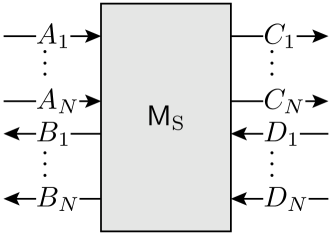
Figure 1: Sketch of the transfer-matrix description of scattering in multi-channel wires.

Assuming current conservation and time reversal symmetry, it is possible to express the transfer matrix of an $N$-channel scatterer in the polar decomposition

$$\mathsf{M}_{\mathrm{S}}=\mathsf{U\Gamma V}$$ (10)

as a product of three matrices, where

$$\mathsf{U} =\begin{pmatrix}\mathsf{u}&0\\ 0&\mathsf{u}^{*}\end{pmatrix},$$ (11)

$$\mathsf{V} =\begin{pmatrix}\mathsf{v}&0\\ 0&\mathsf{v}^{*}\end{pmatrix},$$

$$\mathsf{\Gamma} =\begin{pmatrix}\sqrt{\mathsf{1}+\mathsf{\lambda}}&\sqrt{\mathsf{\lambda}}\\ \sqrt{\mathsf{\lambda}}&\sqrt{\mathsf{1}+\mathsf{\lambda}}\end{pmatrix}\,.$$

$\mathsf{u}$ and $\mathsf{v}$ are complex unitary $N\times N$-matrices, and $\mathsf{\lambda}$ is a real, diagonal $N\times N$-matrix mello91 . The matrix $\mathsf{\lambda}$ contains all transmission probabilities $|t_{a}|^{2}=1/(1+\lambda_{a})$ for the different eigenmodes of the scatterer, where $\lambda_{a}$ is the $a$^th entry of $\mathsf{\lambda}$. Therefore, $\mathsf{\lambda}$ determines the conductance of the scatterer through $g=\sum_{a=1}^{N}1/(1+\lambda_{a})$. The matrices $\mathsf{u}$ and $\mathsf{v}$ describe the way these eigenmodes are connected to the different incoming and outgoing channels. In general, a mixing of channels as illustrated in Figure 2 will occur. The main interest of the polar decomposition consists in the very different rôle played by the radial ($\mathsf{\lambda}$) and angular parameters ($\mathsf{u},\mathsf{v}$), allowing the development of random matrix theories to describe the quantum transport through an arbitrary scatterer been_97 ; jal_95 .

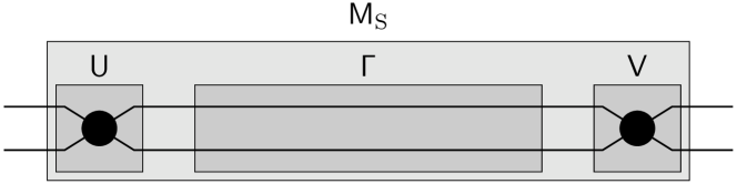
Figure 2: A general transfer matrix $\mathsf{M}_{\text{S}}$ satisfying current conservation and time-reversal symmetry can be expressed as the product (10) of three matrices. $\mathsf{U}$ and $\mathsf{V}$ relate the eigenmodes in the leads to those in the system and $\mathsf{\Gamma}$ describes the transmission and reflection properties of the system.

An $N$-channel ring consisting of a scatterer described by $\mathsf{M}_{\mathrm{S}}$ and an ideal lead can be characterized by the total transfer matrix of the ring $\mathsf{M}_{\mathrm{S}}\mathsf{M}_{\mathrm{L}}$, where $\mathsf{M}_{\mathrm{L}}$ is the diagonal transfer matrix of the lead with entries

$$\left(\mathsf{M}_{\mathrm{L}}\right)_{nn} =\exp{(\mathrm{i}\Phi+\mathrm{i}k_{n}L_{\mathrm{L}})},$$ (12)

$$\left(\mathsf{M}_{\mathrm{L}}\right)_{n+N,n+N} =\exp{(\mathrm{i}\Phi-\mathrm{i}k_{n}L_{\mathrm{L}})}\,,$$

describing right- and left-moving electrons ($1\leq n\leq N$).

The one-particle eigenstates $\psi^{(p)}$ of the ring are defined by the amplitudes $A_{n}^{(p)}$ and $B_{n}^{(p)}$ through the matrix condition

$$(\mathsf{1}-\mathsf{M}_{\mathrm{S}}\mathsf{M}_{\mathrm{L}})\begin{pmatrix}\vec{A}^{(p)}\\ \vec{B}^{(p)}\end{pmatrix}=0\,.$$ (13)

The corresponding eigenenergies $\varepsilon^{(p)}$ satisfy

$$\text{det}(\mathsf{1}-\mathsf{M}_{\mathrm{S}}\mathsf{M}_{\mathrm{L}})=0\,,$$ (14)

where $\mathsf{1}$ denotes the $2N\times 2N$ identity matrix. The contribution $j^{(p)}$ to the persistent current of the ring follows from the flux dependence of $\varepsilon^{(p)}$ through Equation (14). Alternatively, it can also be obtained from the expectation value of the current operator in the leads in the limit of very large $L_{\mathrm{L}}$,

$$j^{(p)}=\frac{e\hbar}{m}\sum_{n=1}^{N}\left(|A_{n}^{(p)}|^{2}-|B_{n}^{(p)}|^{2}\right)\,.$$ (15)

Summing the contributions of all occupied states $p$ we are lead to the persistent current through the ring.

2.2 One-channel scattering problem

For energies $\varepsilon$ between the two lowest transverse energies $\varepsilon_{1}$ and $\varepsilon_{2}$ only one channel propagates and the problem is particularly simple molina04a since $\mathsf{u}$ and $\mathsf{v}$ are pure phases given, respectively, by $\exp[\mathrm{i}(\alpha\pm\zeta)/2]$ in terms of the angles $\alpha$ and $\zeta$. The quantization condition (14) can be written as

$$\cos(\Phi)=\frac{1}{\sin(\theta)\sin(\varphi)}\cos(kL+\delta\alpha)\,.$$ (16)

Following the standard parametrization of a $2\times 2$ transfer matrix molina04a , we have defined the angles $\theta$ and $\varphi$ through

$$\sin(\theta) =\sqrt{\frac{1+\lambda\cos^{2}(\zeta)}{1+\lambda}},$$ (17)

$$\sin(\varphi) =\frac{1}{\sqrt{1+\lambda\cos^{2}(\zeta)}}\,.$$

In this way $t=\exp(\mathrm{i}\alpha)\sin(\theta)\sin(\varphi)$ is the transmission amplitude and $\delta\alpha=\alpha-kL_{\mathrm{S}}$ is the scattering phase-shift. We remark in passing that the expressions simplify in the particular case with right-left symmetry, where $\varphi=\zeta=\pi/2$.

Taking the flux derivative for the $p$-th solution of Equation (16) and following the line of reasoning presented in the appendix of molina04a we obtain the contribution $j^{(p)}$ which after summation over the occupied states leads to (3). For the particular case of $\Phi=\pi/2$ we have molina04a

$$j^{(p)}(\pi/2)=(-1)^{p}\ \frac{e\hbar}{Lm}\ k^{(p)}|t(k^{(p)})|\,.$$ (18)

The alternative route through the eigenvectors is also simple in the $N=1$ case since Equation (15) becomes

$$j^{(p)}=\frac{e\hbar}{mL}\ k^{(p)}\left(\frac{1-|\chi^{(p)}|^{2}}{1+|\chi^{(p)}|^{2}}\right)\,,$$ (19)

with

$$|\chi^{(p)}|^{2} =\left|\frac{B_{1}^{(p)}}{A_{1}^{(p)}}\right|^{2}=\frac{1}{1-\sin^{2}(\theta)\sin^{2}(\varphi)}$$ (20)

$$\times\big{[}1+\sin^{2}(\theta)\sin^{2}(\varphi)-2\sin^{2}(\theta)\sin^{2}(\varphi)\cos^{2}(\Phi)-$$

$$\hphantom{\times\big{[}}2\sin(\theta)\sin(\varphi)\sin(\Phi)$$

$$\hphantom{\times\big{[}}\times\sin\left[\pm\mathrm{arccos}{(\sin(\theta)\sin(\varphi)\cos(\Phi))}\right]\big{]},$$

where the $\pm$ refers to the parity of the eigenstate label $p$. Using

$$|\chi^{(p)}|^{2}_{\Phi=\pi/2}=\frac{(1\mp\sin(\theta)\sin(\varphi))^{2}}{1-\sin^{2}(\theta)\sin^{2}(\varphi)}$$ (21)

in Equation (19) we are lead to the contribution (18) to the persistent current.

2.3 Two-channel scattering problem

For energies $\varepsilon$ satisfying $\varepsilon_{2}<\varepsilon<\varepsilon_{3}$, we have two propagating channels and the matrices $\mathsf{u}$, $\mathsf{v}$ and $\mathsf{\lambda}$ appearing in (11) can be parametrized as

$$\mathsf{u} =\begin{pmatrix}\cos(\varphi)\mathrm{e}^{\mathrm{i}\alpha}&\sin(\varphi)\mathrm{e}^{\mathrm{i}(\alpha+\beta)}\\ -\sin(\varphi)\mathrm{e}^{\mathrm{i}\gamma}&\cos(\varphi)\mathrm{e}^{\mathrm{i}(\gamma+\beta)}\end{pmatrix},$$ (22)

$$\mathsf{v} =\begin{pmatrix}\mathrm{i}\cos(\psi)\mathrm{e}^{\mathrm{i}\epsilon}&-\mathrm{i}\sin(\psi)\mathrm{e}^{\mathrm{i}\theta}\\ -\mathrm{i}\sin(\psi)\mathrm{e}^{\mathrm{i}(\epsilon+\eta)}&-\mathrm{i}\cos(\psi)\mathrm{e}^{\mathrm{i}(\theta+\eta)}\end{pmatrix},$$

$$\mathsf{\lambda} =\begin{pmatrix}\lambda_{1}&0\\ 0&\lambda_{2}\end{pmatrix},$$

where $\lambda_{i}=r_{i}^{2}/t_{i}^{2}$, with $0\leq t_{i},r_{i}\leq 1$ and $t_{i}^{2}+r_{i}^{2}=1$. The mixing angle $\varphi$ introduced here should not be confused with the angle $\varphi$ introduced above for the one-channel case.

The quantization condition (14) can now be written as

$$2\cos^{2}(\Phi)-\text{Tr}\{\mathsf{M}\}\cos(\Phi)+F(\mathsf{M})-1=0\,,$$ (23)

where $\mathsf{M}=\mathsf{M}_{\mathrm{S}}\mathsf{M}_{\mathrm{L}}(\Phi=0)$ and $F(\mathsf{M})$ is given by the $2\times 2$ sub-determinants of $\mathsf{M}$ as

$$F(\mathsf{M})=\text{Re}\sum_{j=2}^{4}\begin{vmatrix}M_{11}&M_{1j}\\ M_{j1}&M_{jj}\end{vmatrix}\ .$$ (24)

Assuming a parabolic dispersion relation in the leads, $k_{1}$ and $k_{2}$ are related by $\hbar^{2}(k_{1}^{2}-k_{2}^{2})/2m=\varepsilon_{2}-\varepsilon_{1}=\Delta\varepsilon$. Defining $k=(k_{1}+k_{2})/2$ we have $k_{1}-k_{2}=m\Delta\varepsilon/\hbar^{2}k$ and the quantization condition (23) at $\Phi=\pi/2$ can be expressed as

$$F(k,L_{\mathrm{L}},t_{1},t_{2},\varphi,\alpha,\beta,\gamma,\psi,\epsilon,\eta,\theta)=1\,.$$ (25)

The allowed $k^{(p)}$ define the eigenstates of the ring, with associated persistent currents

$$j^{(p)}(\pi/2)=\frac{e\hbar k^{(p)}}{m}\left.\left(\frac{\text{Tr}\{\mathsf{M}\}}{\text{d}F/\text{d}k}\right)\right|_{k=k^{(p)}}\,.$$ (26)

In Appendix A we give the expressions of $\text{Tr}\{\mathsf{M}\}$ and $F(\mathsf{M})$ in terms of $k_{1}\pm k_{2}$, $L_{\mathrm{L}}$, $t_{1,2}$, and the angles characterizing the matrices $\mathsf{u}$ and $\mathsf{v}$. The complexity of such expressions forces us to introduce several simplifications in our problem. The most radical one is to take the two channels as spin-degenerate modes. This approximation is treated in the next section, where we analyze the Hubbard chain and show that most of the complexities of the two-channel problem are not present in this case. In Section 4 we consider a simplified two-channel problem and introduce statistical concepts to extract the transmission coefficients.

3 Conductance of a Hubbard chain

In this section, we consider electron transport in a chain with Hubbard-like electron-electron interactions in a finite segment of the chain. This is a particular case of a two-channel chain where the spin degree of freedom of the electrons gives rise to the two channels. We will show that the embedding method can be applied in this special case in a quite straightforward manner and precise numerical calculations can be carried out.

3.1 Model, conductance and spin-rotation symmetry

The Hamiltonian of the whole system reads

$$H=H_{\mathrm{K}}+H_{\mathrm{U}}\,,$$ (27)

where

$$H_{\mathrm{K}}=-\sum_{i}\sum_{\sigma=\uparrow,\downarrow}(c_{i,\sigma}^{\dagger}c_{i+1,\sigma}^{\phantom{\dagger}}+\text{h.c.})$$ (28)

is the homogeneous kinetic energy part describing electrons in an ideal 1D chain. Here, $c_{i,\sigma}$ annihilates an electron with spin $\sigma$ on site $i$, and we define the energy scale by setting the hopping amplitude equal to one. The interacting region situated on sites 1 to $L_{\mathrm{S}}$ is distinguished from the rest of the chain solely by the presence of the on-site Hubbard interaction

$$H_{\mathrm{U}}=U\sum_{i=1}^{L_{\mathrm{S}}}(\hat{n}_{i,\uparrow}-1/2)(\hat{n}_{i,\downarrow}-1/2)$$ (29)

with strength $U$. Here, $\hat{n}_{i,\sigma}=c_{i,\sigma}^{\dagger}c_{i,\sigma}^{\phantom{\dagger}}$. Thus, our interacting system is a chain of $L_{\mathrm{S}}$ sites on which a spin-up electron interacts with a spin-down electron on the same site.

We fix the Fermi energy in the leads to the center of the band, corresponding to half-filling. The interaction term $H_{\mathrm{U}}$ contains a background potential which renders the system particle-hole symmetric and ensures half-filling in the interacting region independent of the interaction strength.

The two channels in our problem are defined by the two possible orientations of the electron spin $\sigma=\{\uparrow,\downarrow\}$. In the absence of a magnetic field, the corresponding states in the leads are degenerate.

If we are allowed to describe the many-body scattering through the interacting segment of the chain by an effective single-electron scattering situation, the conductance is given by the sum over all effective transmission probabilities as

$$g=\sum_{\sigma,\sigma^{\prime}}\left|t_{\sigma\sigma^{\prime}}\right|^{2}\,,$$ (30)

where $t_{\sigma,\sigma^{\prime}}$ is the transmission amplitude from the incoming channel of spin $\sigma$ into the outgoing channel characterized by spin $\sigma^{\prime}$.

We show in the sequel that spin-rotation symmetry imposes serious limitations on the transmission coefficients. Since the Hamiltonian is invariant under a rotation of the spin basis $\{|{\uparrow}\rangle,|{\downarrow}\rangle\}$, there can be no preferential spin orientation. As a consequence, the transmission matrix must have the same symmetry. Invariance of the transmission matrix $\mathsf{t}$ under arbitrary spin rotations excludes transmissions accompanied by a spin flip so that

$$t_{\uparrow\downarrow}=t_{\downarrow\uparrow}=0\,.$$ (31)

Otherwise the transmission matrix could be diagonalized by a spin rotation thereby violating the spin-rotation symmetry. Furthermore, the transmissions with spin conservation have to be equal

$$t_{\uparrow\uparrow}=t_{\downarrow\downarrow}=t\,.$$ (32)

An alternative way of demonstrating the conditions (31) and (32) is to use the procedure of the reduction to the single-channel scattering. We develop this second path in Appendix B.

3.2 Numerical results for the conductance of Hubbard chains

As discussed in the previous section, the effective one-body scattering describing the transmission through a Hubbard chain is characterized by spin conservation and the two spin channels are not mixed by the effective one-body scatterer. The transmission through the effective scatterer is therefore characterized by a single parameter, the spin-independent transmission amplitude $t$. The conductance (30) then simplifies to

$$g=2\left|t\right|^{2}\,.$$ (33)

This expression holds for arbitrary interaction strength in our Hubbard chain. The spin appears as a factor of two, as in the case of general one-dimensional Fermi liquid systems with spin rejec03 .

The relation between persistent current and effective one-body transmission amplitude which forms the basis of the standard embedding method for the single-channel case can now be generalized to two channels without mixing. The persistent current is then given by the sum of the contributions from the two independent channels. If in addition to the spin-rotation symmetry of the Hamiltonian, we choose a spin-independent filling of the two subsystems with $N_{\uparrow}=N_{\downarrow}$, the two contributions are equal such that the two-channel persistent current is twice the single-channel value. As a consequence, (5) is replaced by

$$|t|=\sin\left(\frac{\pi}{4}\frac{\mathcal{D}_{\infty}^{(2)}}{\mathcal{D}_{\infty}^{0}}\right)\,,$$ (34)

where $\mathcal{D}_{\infty}^{(2)}$ is the numerically obtained two-channel phase sensitivity in the limit of a very large ring. When the ring size is not much larger than the Hubbard chain, the flux dependence of the current may change considerably and reach a very different functional form for $L_{\mathrm{L}}\ll L_{\mathrm{S}}$ waintal08 .

We use the Density Matrix Renormalization Group algorithm (DMRG) white92 ; DMRG_book ; schmitteckert_thesis adapted to the Hubbard model to calculate $\mathcal{D}^{(2)}$ for a two-channel ring with a Hubbard segment, taking fully into account the electronic correlations. These many-body ground state properties are calculated for half-filled rings with increasing sizes $L$ corresponding to odd numbers $N_{\uparrow}=N_{\downarrow}=L/2$ of electrons for each spin channel. We keep up to 6000 states in the DMRG iterations, and perform fits to extrapolate the size-dependence of $\mathcal{D}^{(2)}$ to $D_{\infty}^{(2)}$ vasseur_thesis .

The numerical results for the conductance of short Hubbard chains using (34) are presented in Figure 3. For even $L_{\mathrm{S}}$ we obtain a suppression of the conductance by the interaction that becomes more pronounced for longer Hubbard chains. This can be interpreted as a precursor of the Mott-Hubbard transition. For weak interaction strengths, our numerical results presented in Figure 3 are in agreement with the results of the perturbative approach of Reference oguri01 . However, the perturbative approach does not yield the significant $L_{\mathrm{S}}$-dependence that we obtain at strong interaction. Nevertheless, a strong interaction-induced reduction of the conductance has been obtained for a Hubbard chain of length $L_{\mathrm{S}}$ with reduced coupling to the reservoirs oguri06 .

Figure 3: Conductance of short Hubbard chains as a function of the interaction strength. The solid lines are guide to the eyes. The dashed curve shows the perturbative result produced using the theory of Reference oguri01 .

For odd values of $L_{\mathrm{S}}$ it has been predicted from perturbative arguments oguri99 ; oguri01 and a numerical renormalization group (NRG) study oguri05 that the transmission should be perfect. As shown in Figure 3, this perfect conductance $g=2$ is found in the case of a single Hubbard impurity $L_{\mathrm{S}}=1$. For other odd numbers of interacting Hubbard sites, our results at strong interaction show small deviations from $g=2$ (see Table 1 for the $L_{\mathrm{S}}=3$ case). These deviations are of the order of the uncertainty of the extrapolation procedure included in the embedding method. It is then important to develop complementary approaches to test, and eventually improve, these values. This task is undertaken in the next two subsections.

3.3 Numerical limitations of the standard embedding method

As mentioned in the introduction, the curvature yields an alternative route for extracting the absolute value of the transmission amplitude. In the two-channel case, Equation (7) becomes

$$\mathcal{C}_{\infty}^{(2)}=\frac{2e^{2}v_{\mathrm{F}}}{\pi\hbar}\frac{|t|\arccos(|t|)}{\sqrt{1-|t|^{2}}}\,.$$ (35)

In order to verify that the many-body two-channel scatterer modelled by a chain with Hubbard-like electron-electron interactions can indeed be replaced by the effective one-body scatterer without channel mixing described in the previous section, we compute the transmission from the curvature $\mathcal{C}_{\infty}^{(2)}$ schmitteckert04 and compare it with the one obtained from the phase sensitivity $\mathcal{D}_{\infty}^{(2)}$. Since the latter is a measure for the integral of the persistent current over the flux interval $0\leq\Phi\leq\pi$, and the former corresponds to the slope of the increase of the persistent current as a function of flux at $\Phi=0$, $\mathcal{D}_{\infty}^{(2)}$ and $\mathcal{C}_{\infty}^{(2)}$ characterize very different aspects of the persistent current and its dependence on the flux. The two quantities are related to the transmission of an effective one-body scatterer by the relations (34) and (35). If the many-body scatterer can be characterized by an effective one-body scatterer, then the flux dependence of the persistent current in the correlated system has to agree with the one of a ring with an effective one-body scatterer, and the two alternative ways of extracting $|t|$ should be equivalent. This is the case for even $L_{\mathrm{S}}$, where the results obtained from (35) are very close to the ones resulting from the phase sensitivity shown in Figure 3. The strongest deviations are of the order of 2 %, which is smaller than the symbol size. For odd $L_{\mathrm{S}}$, the results of Table 1 show a difference between the two methods for large values of the interaction strength. However, these differences are of the order of the deviation from the expected result of perfect transmission. Therefore, we can conclude that the two methods agree within their precision. The consistency of the values of $|t|^{2}$ extracted from $\mathcal{D}_{\infty}^{(2)}$ and $\mathcal{C}_{\infty}^{(2)}$ can then be considered as strong evidence for the validity of the embedding method.

Table 1: Values of the effective transmission probability $|t|^{2}$ for a Hubbard chain of length $L_{\mathrm{S}}=3$ obtained from the embedding method using the phase sensitivity (first line) and the curvature (second line), for different values of the interaction strength $U$. The last line is the result of a two-parameter fit to the flux dependence obtained using damped boundary conditions.

	$U=0$	$U=2$	$U=4$	$U=6$
from $\mathcal{D}$	1.00	1.00	0.98	0.75
from $\mathcal{C}$	1.00	0.99	0.95	0.65
damped boundary		0.9996	0.996	0.968

Figure 4: Persistent currents extrapolated to infinite lead length as a function of the magnetic flux for a ring containing a Hubbard chain with $L_{\mathrm{S}}=3$ and $U=6$ (squares). The error bars indicate the difference between a linear and a parabolic extrapolation of the available data. The line is a fit of (3) to the data points yielding $|t|^{2}\approx 0.87$.

For the most critical case of Table 1 ($U=6$) we have performed the numerically very demanding calculation of the persistent currents for different values of the flux. The numerical data extrapolated to infinite lead length are shown in Figure 4. The uncertainty of the extrapolations indicated by the errorbars remains unfortunately rather important. The one-parameter fit of (3) (with an additional factor of 2 for the spin) to the data points yields $|t|^{2}\approx 0.87$, much closer to the expected perfect transmission than the values extracted from $\mathcal{D}_{\infty}^{(2)}$ and $\mathcal{C}_{\infty}^{(2)}$ shown in Table 1.

In comparison with the single-channel case, the correlated two-channel scattering problem requires considerably higher numerical efforts at equal ring length. As a consequence, we had to limit our computations to total ring sizes $L\leq 30$. As discussed above, this is not generally a problem, but it affects the quality of the extrapolations to infinite ring size for situations close to conductance resonances molina04a , such as the case of half filling and odd values of $L_{\mathrm{S}}$. The reliability of the extrapolations of the numerically obtained values to infinite lead length becomes limited when the energy resolution given by the level spacing in the largest rings is insufficient to resolve the resonance at the band center, whose width strongly decreases with increasing odd $L_{\mathrm{S}}$ and $U$. In order to overcome this problem, considerably larger ring sizes would have to be considered to improve the extrapolations. However, it appears impossible within the standard embedding method, and with the present computational resources, to perform precise enough calculations for sufficiently large ring sizes. In the next subsection we develop an improved embedding method that allows to overcome these difficulties.

3.4 Improved embedding method: Damped boundary conditions

In order to overcome the limitation in ring size, we introduce damped boundary conditions bohr06 that allow to simulate longer effective lead lengths. The damped boundary conditions consist in a reduction of the last $L_{\mathrm{D}}$ hopping elements of the Hamiltonian on both sides of the Hubbard chain, leading to a region with reduced local bandwidth in the ring opposite to the Hubbard part, as indicated in Figure 5 by the distance between the upper and the lower line. The increased local density of states is reminiscent of a long lead having full hopping values. We choose an exponential reduction controlled by a damping parameter $\Lambda<1$ such that the last hopping elements on either side of the interacting region are given by $\Lambda^{j}$ with $j$ counting the last $L_{\mathrm{D}}$ sites.

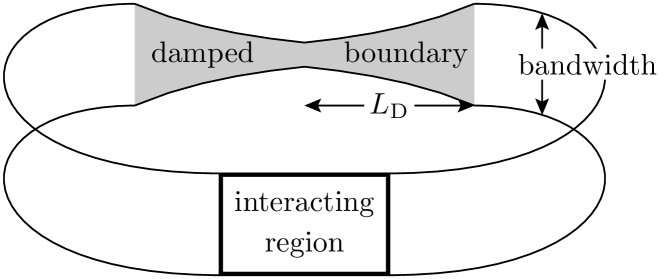
Figure 5: Sketch of the damped boundary condition setup. The hopping matrix elements are exponentially reduced on the $L_{\mathrm{D}}$ last sites on both sides of the interacting region, locally suppressing the bandwidth as indicated by the distance between the upper and lower line. The increased density of states in the damped boundary region simulates an effectively longer lead.

Figure 6: Persistent currents as a function of flux for half-filled Hubbard rings with $L=30$ and $L_{\mathrm{S}}=3$. Data points are obtained using damped boundary conditions with $L_{\mathrm{D}}=10$ and damping $\Lambda=0.7$. Crosses, pluses, and squares are for interaction strengths $U=2$, 4, and 6, respectively. The lines are two-parameter fits of the formula (3) yielding the values of Table 1 for the transmission and effective lengths $L_{\mathrm{eff}}=278$, 282, and 295, respectively.

We have checked that for the cases of Figure 3 the results using damped boundary conditions reproduce those from the reliably extrapolated standard embedding method. However, the usefulness of the improved method appears in the cases previously discussed where the standard embedding method meets its numerical limitations. We therefore show in Figure 6 numerical results for the persistent currents using damped boundary conditions for $L_{\mathrm{S}}=10$, with $L_{\mathrm{D}}=10$ and $\Lambda=0.7$. The lines are fits of the analytical result for the persistent current of noninteracting particles without damped boundary conditions (formula (3) with an additional factor of 2 for the spin). The transmission of the scatterer and the effective length of the ring have been used as fitting parameters. The quality of the fits is a strong indication for the validity of the embedding method in the Hubbard model case since it provides a comparison of the flux dependence with that of the noninteracting case as it was done for the single-channel case molina04a .

The fitting parameters show indeed that the effective lead length can increase considerably with the damping, provided it is not chosen too strong. Damping parameters larger than $\Lambda=0.7$ result, for the system parameters chosen here, in backscattering, and therefore render the reliability of the extracted conductances questionable. Remarkably, the resulting transmission approaches the expected perfect conductance (see Table 1). Thereby we have obtained a considerable improvement from the standard extrapolation procedure, in particular for cases where the latter yields poor results. The results of the improved embedding method can thus be considered to be consistent with the perfect conductance for all odd values of $L_{\mathrm{S}}$ that is expected from perturbative arguments oguri99 ; oguri01 and NRG oguri05 .

4 Persistent currents for two degenerate channels

In the previous section we considered the case of degenerate and uncoupled channels, where the generalization of the one-dimensional embedding method is rather straightforward. Once we take into account channel mixing, the one-to-one correspondence between persistent currents and transmission coefficients is lost. However, we still expect that the $\lambda$ parameters of the polar decomposition (10) will be determining the corresponding persistent currents. We will treat in this section an arbitrary channel mixing, and in order to keep the problem tractable we consider quasi-degenerate channels, where $|k_{1}-k_{2}|\ll k$. In this case, if we neglect the weak $k$-dependence of $\mathsf{u}$, $\mathsf{v}$, and $\mathsf{\lambda}$, the solutions of (25) are doubly degenerate, since the rôles of $A_{1}^{(p)}$ and $A_{2}^{(p)}$ (or $B_{1}^{(p)}$ and $B_{2}^{(p)}$) are interchangeable.

4.1 Symmetric nanosystems with fixed channel mixing

In the case where the nanosystem exhibits left-right inversion symmetry we can set $\alpha=\epsilon$, $\beta=\eta$, $\gamma=\theta$, and $\varphi=\psi$ in (22). This assumption considerably simplifies the expression of $\text{Tr}\{\mathsf{M}\}$ and $F(\mathsf{M})$ presented in Appendix A, and thus the resulting analytical calculations.

Even in the symmetric case the problem is still rather complicated. We therefore consider particular values of $\varphi$. For instance, for $\varphi=0$, (25) leads to

$$\cos(2[kL_{\mathrm{L}}+\alpha+\beta+\gamma])=\cos(2[\alpha-\beta-\gamma])$$ (36)

and one gets two families of solutions

$$k^{(\ell,1)}L_{\mathrm{L}}= -2\alpha+\ell\pi$$ (37)

$$k^{(\ell,2)}L_{\mathrm{L}}= -2(\beta+\gamma)+\ell\pi\,.$$

Using (26), these quantized $k$-values lead to the single-levels currents

$$j^{(\ell,b)}=(-1)^{\ell}\frac{e\hbar}{mL_{\mathrm{L}}}k^{(\ell,b)}|t_{b}|\quad b=1,2\,,$$ (38)

Choosing $\varphi=\pi/2$, one gets similar results with an interchange of $t_{1}$ and $t_{2}$, and a relative sign between the two current contributions. The fact that the persistent currents associated with the ring eigenmodes are solely determined by the transmission eigenvalues is to be expected since for these particular values of $\varphi$ there is no mode-mixing by $\mathsf{M}$.

A more interesting case is that of $\varphi=\pi/4$, which corresponds to the maximum mode-mixing and the most likely value if we take the matrix $\mathsf{u}$ as uniformly distributed in the unitary ensemble been_97 . The corresponding quantization condition is

$$k^{(\ell,b)}L_{\mathrm{L}}=-\alpha-\beta-\gamma+\frac{(-1)^{b}}{2}{\rm arccos}(\chi)+\ell\pi$$ (39)

with

$$\chi =\Delta\sin^{2}(\alpha-\gamma)+\cos^{2}(\alpha-\gamma)\cos(2\beta)\,,$$ (40)

$$\Delta =t_{1}t_{2}-r_{1}r_{2}\,.$$ (41)

The resulting persistent currents are given by

$$j^{(\ell,b)}= (-1)^{\ell+1}\frac{e\hbar k^{(\ell,b)}}{2mL_{\mathrm{L}}}\mathrm{sgn}[\cos(\alpha-\gamma)]$$ (42)

$$\times \left\{\frac{(t_{2}-t_{1})\mathrm{sgn}[\cos(\beta)]}{\sqrt{1+\frac{1+\Delta}{2\cos^{2}(\beta)}\tan^{2}(\alpha-\gamma)}}\right.$$

$$\left.+(-1)^{b}\frac{(t_{1}+t_{2})\mathrm{sgn}[\sin(\beta)]}{\sqrt{1+\frac{1-\Delta}{2\sin^{2}(\beta)}\tan^{2}(\alpha-\gamma)}}\right\}\,,$$

and therefore are bounded by

$$\left|j^{(\ell,b)}\right|\leq\frac{e\hbar k^{(\ell,b)}}{mL_{\mathrm{L}}}\max\{t_{1},t_{2}\}\,.$$ (43)

In the limit of large $L_{\mathrm{L}}$ we can take $k^{(\ell,1)}\simeq k^{(\ell,2)}\simeq k^{(\ell)}=\ell\pi/L_{\mathrm{L}}$ and show that

$$\left|j^{(\ell,1)}+j^{(\ell,2)}\right| \leq\frac{e\hbar k^{(\ell)}}{mL_{\mathrm{L}}}\left|t_{1}-t_{2}\right|\,,$$ (44)

$$\left|j^{(\ell,1)}-j^{(\ell,2)}\right| \leq\frac{e\hbar k^{(\ell)}}{mL_{\mathrm{L}}}\left(t_{1}+t_{2}\right)\,.$$ (45)

We remark that, leaving aside the trivial case of uncoupled channels, the relationship between persistent current and transmission amplitudes is not unique, as it involves the mixing angles. However, already the special case $\varphi=\pi/4$ shows that there are stringent constraints on the possible values of $t_{1}$ and $t_{2}$. If we disposed of an ensemble of different scatterers with fixed $t_{1}$, $t_{2}$, and mixing angle $\varphi$, we could extract the transmission amplitudes by varying the angles $\alpha$, $\beta$ and $\gamma$ through the ensemble. We carry on this procedure by choosing these three angles uniformly distributed in the interval $(0,2\pi)$, solving the resulting eigenvalue problem (13), and then obtaining from (15) the two resulting persistent currents. For $\varphi=\pi/4$ we obtain the distribution of normalized persistent currents $\hat{\jmath}^{(1,2)}=mL_{\mathrm{L}}/(e\hbar|k|)j^{(1,2)}$ shown in Figure 7, where we have arbitrarily taken $t_{1}=0.8$ and $t_{2}=0.4$. The restrictions imposed by (44) and (45) constrain the possible values of $(\hat{\jmath}^{(1)},\hat{\jmath}^{(2)})$ to the rectangle defined by $(\pm t_{1,2},\mp t_{2,1})$. The rectangle $(\pm t_{1,2},\pm t_{2,1})$ appears because the chosen pairs $(\hat{\jmath}^{(1)},\hat{\jmath}^{(2)})$ do not necessarily have the same $\ell$, as was the case in (42). Interestingly, the $(\hat{\jmath}^{(1)},\hat{\jmath}^{(2)})$ distribution is quite non-uniform, but concentrated around $(0,0)$ and, in particular, at the vertices of the rectangles.

Other mixing angles are difficult to deal with at the analytical level, but the $(\hat{\jmath}^{(1)},\hat{\jmath}^{(2)})$ distribution can be obtained as in the previous case. This is done in Figure 8 for $\varphi=\pi/8$, and with the same values of $t_{1}$ and $t_{2}$ as before. We see that the restrictions (44) and (45) still apply, the distribution is depleted around the central point $(0,0)$, and the concentration around the vertices of the rectangles is more pronounced than for the case of $\varphi=\pi/4$. In Figure 9 we present the probability distribution of $(\hat{\jmath}^{(1)},\hat{\jmath}^{(2)})$ as a function of the angle $\varphi$. Considering different horizontal cross-sections, like Figures 7 and 8, we can follow the evolution from the uncoupled channel case to that of intermediate mixings.

4.2 Asymmetric nanosystems and random channel mixing

In the previous subsection we have seen that in the case of left-right inversion symmetry the transmission amplitudes can be inferred from the study of the distribution of matrices $\mathsf{M}$ with fixed radial parameters $\lambda_{1,2}$ and varying angular parameters. This procedure can be formalized by taking a random matrix approach for the $\mathsf{u}$ and $\mathsf{v}$ matrices, while keeping $\mathsf{\Gamma}$ fixed. This kind of approach is widely used in the application of random matrix theory to quantum transport, where we separate the statistics of the matrices $\mathsf{u}$ and $\mathsf{v}$ from that of the transmission eigenvalues. While the first ones are assumed to be uniformly distributed over the unitary ensemble, the distribution of the latter depends on the nature of the problem under study, i.e. its diffusive or chaotic character jal_95 . In practice, such a method would require to connect the nanosystem under study to mode-mixing reflectionless diffusors, represented by matrices uniformly distributed on the unitary ensemble, and to study the resulting distribution of persistent currents.

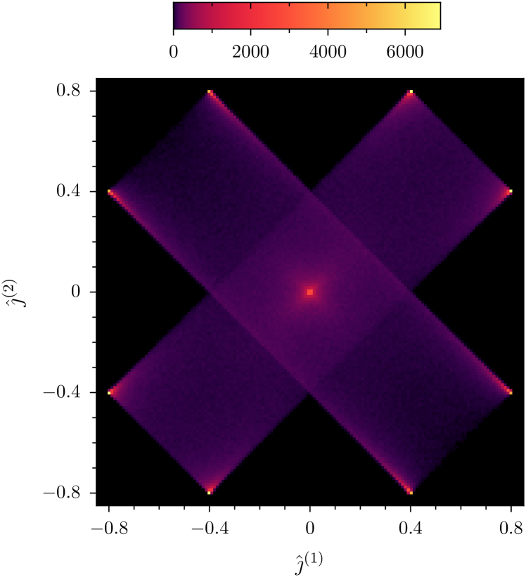
Figure 7: Color scale plot of the distribution $(\hat{\jmath}^{(1)},\hat{\jmath}^{(2)})$ for $t_{1}=0.8$ and $t_{2}=0.4$ in the case of a left-right symmetric scatterer with a channel mixing angle $\varphi=\pi/4$.

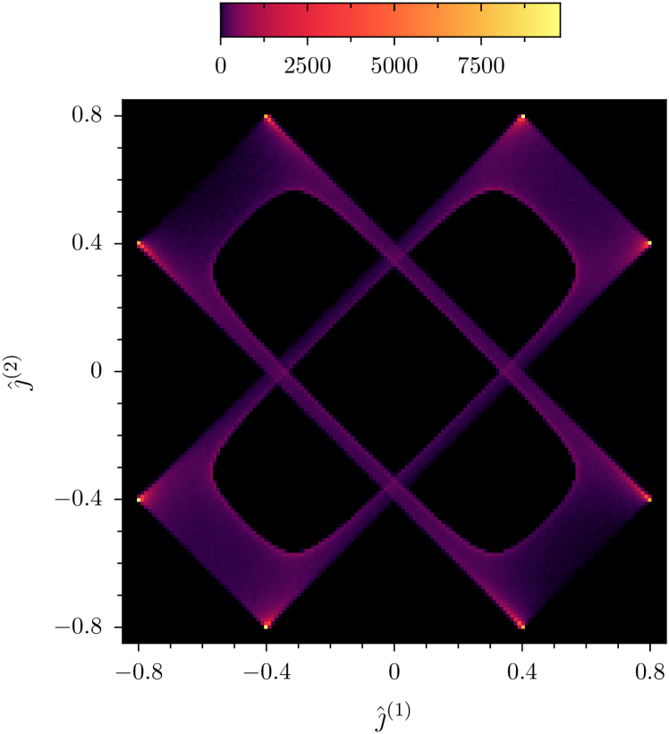
Figure 8: Color scale plot of the distribution $(\hat{\jmath}^{(1)},\hat{\jmath}^{(2)})$ for $t_{1}=0.8$ and $t_{2}=0.4$ in the case of a left-right symmetric scatterer with a channel mixing angle $\varphi=\pi/8$.

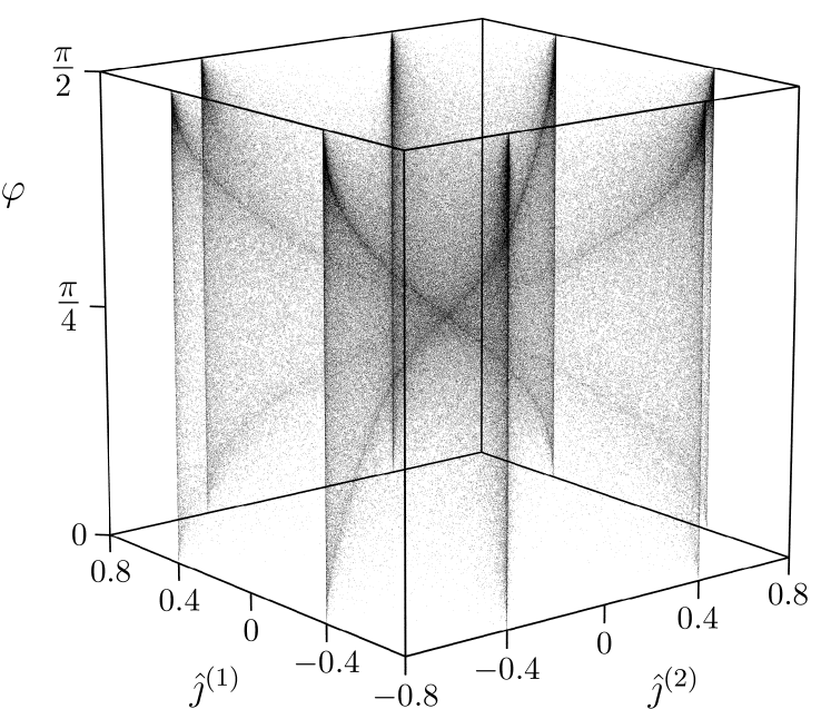
Figure 9: Probability density to find a pair $(\hat{\jmath}^{(1)},\hat{\jmath}^{(2)})$ for $t_{1}=0.8$ and $t_{2}=0.4$ with left-right symmetry as a function of the mixing angle $\varphi$ (vertical axis).

Since our procedure will be carried out numerically, we can drop the symmetry requirement of the previous subsection. We then generate a large number of independent unitary matrices $\mathsf{u}$ and $\mathsf{v}$ for fixed transmission amplitudes $t_{1}$ and $t_{2}$. The two non-degenerate $k$-values arising from the quantization condition (25) for $\Phi=\pi/2$ yield pairs of normalized persistent currents $\hat{\jmath}^{(1)}$ and $\hat{\jmath}^{(2)}$, that we obtain from Equation (15). The resulting distribution is presented in Figure 10. Comparing with Figure 9, there are some differences since we do not have spatial symmetry and the angle $\varphi$ is averaged over the unitary ensemble. However, similar information can be extracted from both cases: the transmission amplitudes appear as the bounds and the most likely values of the $(j^{(1)},j^{(2)})$ distribution.

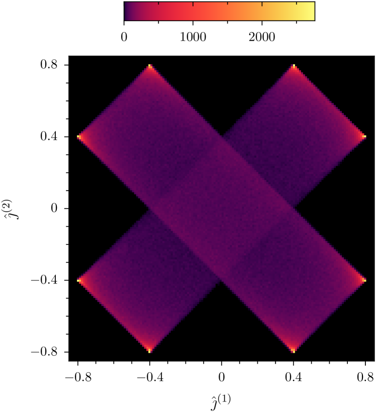
Figure 10: Color scale plot of the probability density to find a pair $(\hat{\jmath}^{(1)},\hat{\jmath}^{(2)})$ for $t_{1}=0.8$ and $t_{2}=0.4$ with random channel mixing.

Figure 11: Probability distribution $p(\hat{\jmath})$ of the normalized total persistent current $\hat{\jmath}$ in a ring containing a two-channel scatterer with random channel mixing for $t_{1}=0.8$ and $t_{2}=0.2$ (solid line), $0.4$ (dashed), $0.6$ (dotted) and $0.8$ (dashed-dotted).

If we now consider a non-interacting many-particle system, the sum over the occupied levels should be carried out in order to obtain the total persistent current. Assuming that, like in the $N=1$ case, the total persistent current is dominated by the contribution at the Fermi level, it is of interest to consider the distribution of the sum $\hat{\jmath}=\hat{\jmath}^{(1)}+\hat{\jmath}^{(2)}$. Such a distribution is presented in Figure 11 on a logarithmic scale for $t_{1}=0.8$ and various values of $t_{2}\leq t_{1}$. The structure found in Figure 10 translates into bounds of $\hat{\jmath}$ at $\pm(t_{1}+t_{2})$ and strong peaks at $\pm|t_{1}-t_{2}|$. Therefore, from the distribution of $\hat{\jmath}$ when branching the nanosystem to random reflectionless diffusors we can infer the values of the amplitudes $t_{1}$ and $t_{2}$, and eventually the conductance of the system.

The relationships that we have found between persistent currents and transmission amplitudes in the non-interacting two-channel case are interesting, but difficult to use in a practical way. The extension beyond $N=2$ is in principle possible. However, as $N$ grows it becomes increasingly difficult to identify the $N$ transmission eigenvalues from the distribution of $\hat{\jmath}=\sum_{b=1}^{N}\hat{\jmath}^{(b)}$. Our main interest is in the $N=2$ case once the interactions are switched on. The use of the statistical approach for the interacting case, leaving practical considerations aside, would rely on three key assumptions. Firstly, like in the $N=1$ case, we have to accept that the interacting problem is described by effective one-particle scattering parameters. Secondly, the total persistent current should be dominated by its Fermi level contribution. Lastly, the two channels at the Fermi level need to be quasi-degenerate.

5 Reduction of multi-channel scattering to single-channel problems

As we have seen in the previous section, it is not obvious how to extract the transmission probabilities of an $N$-channel scatterer required for the calculation of the conductance from the persistent current distribution of an $N$-channel ring. However, it is possible to calculate several single-channel persistent currents which then allow in principle to characterize completely the many-channel scattering matrix.

The effective one-channel scattering problem $ij$ is obtained by connecting two channels $i$ and $j$ which both can be situated on either side of the scattering region. All other channels are closed by reinjecting the outgoing current into the scattering region. For the example of two channels we present in Figure 12 the six different possible setups. Note that the noninteracting ring does not necessarily connect opposite sides of the interacting region. In principle, the electrons can acquire an arbitrary phase upon injection. While this phase may represent a useful tool, we will set it to zero in the sequel. For an $N$-channel problem one can construct in this way $2N^{2}-N$ different one-channel scattering problems.

Figure 12: For a two-channel scattering problem there exist six different one-channel scattering problems which can be treated with the standard embedding method.

Within the embedding method, the effective one-channel setup linking channels $i$ and $j$ has an associated persistent current from which the modulus $T_{ij}$ of the corresponding transmission amplitude can be determined. Clearly, the $T_{ij}$ are functions of the $2N^{2}+N$ parameters defining the matrices $\mathsf{u}$, $\mathsf{v}$, and $\mathsf{\lambda}$. Such functions are presented in the appendix for the two-channel case. In the general case, we have $2N^{2}-N$ different $T_{ij}$, so that $2N$ irrelevant phases are left undetermined.

Our goal is to extract the radial parameters $\lambda_{a}$ that determine the conductance. Already the application of the embedding method to all of the $2N^{2}-N$ one-channel problems may require considerable numerical resources and the procedure might be quite lengthy. In addition, the complicated functional dependence of the $T_{ij}$ makes obtaining the $\lambda_{a}$ a challenging task. Depending on the symmetries of the system under investigation, both the number of parameters appearing in the transfer matrix and the number of nonequivalent one-channel problems may be reduced with respect to these general expressions.

Furthermore, interaction-induced nonlocal effects impose some restrictions. For the effective transmission of interacting one-dimensional scatterers, it has been found that the usual composition law of scatterers in series does not hold molina05 ; weinmann08 . The deviations can be interpreted as a nonlocal interaction-induced effect on the effective transmission of an interacting scatterer. This effect disappears only in the limit of large distance between the scatterers. In the present situation, the closing of channels might represent a perturbation leading to such a nonlocal effect unless the connecting leads are sufficiently long.

Despite these difficulties the proposed method might provide a possible approach for the demanding problem of many-body transport with mixing channels. For instance, we might study larger Hubbard chains than the ones we have addressed with the other methods. In addition, the fact of separating the problem into single-channel setups can be useful for the general analysis of the multi-channel scattering case as will be exemplified in Appendix B.

6 Conclusions

The embedding method for extracting the conductance of an interacting nanosystem is by now a well established and widely used procedure in the case of one-dimensional spinless fermions favand98 ; sushkov01 ; molina03 ; meden03 ; rejec03 ; molina04a ; molina05 . Its validity has been ascertained and interesting physical phenomena have been found from its application molina04a ; molina05 ; vasseur_thesis . The extension of the embedding method to the case of two channels is therefore of great importance. In this work we have presented various possible extensions of the $N=1$ embedding method to $N=2$, depending on the nature of the channels.

When the channels represent the two spin directions, we have a one-dimensional Hubbard chain, where the absence of an effective spin-flip term allows for a straightforward generalization of the $N=1$ embedding method. The use of the DMRG algorithm in the presence of spin makes the problem numerically demanding, but we have checked that the method is reliable for chains of up to 4 interacting sites. We have introduced an improvement of the standard embedding method by considering damped boundary conditions, allowing to address larger systems and to deal with resonances, which is the case for an odd number of interacting sites $L_{\mathrm{S}}$. Our results are compatible with the perfect conductance predicted for a Hubbard chain with an odd number of sites oguri99 . For even $L_{\mathrm{S}}$ the conductance is reduced by the electron-electron interactions. Similar qualitative behavior has been established for Hubbard chains coupled to reservoirs using NRG oguri05 .

The generalization of the embedding method to the case of two mixed channels is difficult due to the increased number of transmission amplitudes that are necessary to determine the conductance. In the case of quasi-degenerate channels, by connecting different pairs of channels we reduce the problem to various one-dimensional setups, where the corresponding transmission amplitude can be obtained from the associated persistent current. The implementation of such a method requires considerable numerical resources and solving a system of eight coupled non-linear equations. In the non-interacting case with quasi-degenerate channels we proposed a statistical approach that leads to the values of the transmission amplitudes from the distribution of persistent currents obtained while varying the mixing of the channels. The practical implementation of this method in order to extract the conductance of a given nanosystem would rely in coupling it with an ensemble of reflectionless diffusors that scramble the phases of the transfer matrix without affecting the transmission amplitudes.

The embedding method is based on an effective one-particle description of a correlated system. Anderson-like quantum impurity models like that of a short Hubbard chain scattering conduction electrons or the Interacting Resonant Level Model mehta06 ; doyon07 ; boulat08 have been studied in the literature through the numerical renormalization group (NRG) hewson_book ; oguri05 or the Bethe-Ansatz mehta06 ; doyon07 ; boulat08 . From these studies we know that the low-energy excitations behave like free fermions in the zero-temperature limit of those models. This is the case in régimes where the effect of interactions remains perturbative, as well as in the non-perturbative limit. In this latter limit, where (spin or orbital) Kondo effects occur, the extended conduction electrons continue to behave as free fermions below the Kondo temperature, as first shown by Wilson hewson_book .

Extending this concept to arbitrary interacting nanosystems, one can justify the assumption that an interacting region embedded between non-interacting leads can still be described at sufficiently low temperatures and sufficiently far away as an effective one-body scatterer with interaction-dependent effective parameters. In certain studies of quantum impurity models, the effective quantum transmission is extracted directly from the knowledge of the effective one-body excitations or, via the Friedel sum rule, from the knowledge ng88 ; freyn10 of the occupation numbers of the interacting region.

Although, not surprisingly, many-channel problems require a larger numerical effort, the extension of the embedding method to more than one channel is feasible and we have presented several ideas to achieve this generalization. The embedding method is thus available for future practical applications beyond the one-channel case.

Appendix A Formulas for the two-channel problem

In this appendix we present the explicit form of $\text{Tr}\{\mathsf{M}\}$ and $F(\mathsf{M})$, which are necessary for solving the quantization condition (23) of the two-channel problem. We are interested in expressing them in terms of $k_{1}\pm k_{2}$. For the former we have

$$\text{Tr}\{\mathsf{M}\}=T^{1/2}\big{[} \cos(k_{1}L_{\mathrm{L}}-\xi_{1})\cos(\Omega)$$ (46)

$$+\cos(k_{2}L_{\mathrm{L}}-\xi_{2})\sin(\Omega)\big{]}\,,$$

with

$$\frac{T}{4}= \frac{1+\cos(2\varphi)\cos(2\psi)}{2}\left(\frac{1}{t_{1}^{2}}+\frac{1}{t_{2}^{2}}\right)$$ (47)

$$-\frac{1}{t_{1}t_{2}}\sin(2\varphi)\sin(2\psi)\cos(\beta+\eta)\,,$$

$$\tan{\xi_{1}} =$$ (48)

$$\frac{t_{1}\tan(\varphi)\tan(\psi)\cos(\alpha+\beta+\epsilon+\eta)-t_{2}\cos(\alpha+\epsilon)}{t_{1}\tan(\varphi)\tan(\psi)\sin(\alpha+\beta+\epsilon+\eta)-t_{2}\sin(\alpha+\epsilon)}\,,$$

$$\tan{\xi_{2}} =$$ (49)

$$\frac{t_{1}\cos(\gamma+\beta+\theta+\eta)-t_{2}\tan(\varphi)\tan(\psi)\cos(\gamma+\theta)}{t_{1}\sin(\gamma+\beta+\theta+\eta)-t_{2}\tan(\varphi)\tan(\psi)\sin(\gamma+\theta)}\,,$$

$$\tan^{2}{\Omega} =$$ (50)

$$\frac{t_{1}^{2}+t_{2}^{2}\tan^{2}(\varphi)\tan^{2}(\psi)-2t_{1}t_{2}\tan(\varphi)\tan(\psi)\cos(\beta+\eta)}{t_{1}^{2}\tan^{2}(\varphi)\tan^{2}(\psi)+t_{2}^{2}-2t_{1}t_{2}\tan(\varphi)\tan(\psi)\cos(\beta+\eta)}\,.$$

The evaluation of (24) yields

$$F(\mathsf{M})=\frac{1+\cos(2\varphi)\cos(2\psi)}{2}$$ (51)

$$-\frac{\sin(2\varphi)\sin(2\psi)[\cos(\beta+\eta)-r_{1}r_{2}\cos(\beta-\eta)]}{2t_{1}t_{2}}$$

$$+\frac{\cos([k_{1}+k_{2}]L_{\mathrm{L}}+\alpha+\beta+\gamma+\epsilon+\eta+\theta)}{t_{1}t_{2}}$$

$$+\frac{\sin(2\varphi)\sin(2\psi)\cos([k_{1}-k_{2}]L_{\mathrm{L}}+\alpha+\epsilon-\gamma-\theta)}{2}$$

$$-\frac{1}{2t_{1}t_{2}}\big{(}\cos([k_{1}-k_{2}]L_{\mathrm{L}}+\alpha+\epsilon-\gamma-\theta)$$

$$\quad\times[(1+\cos(2\varphi)\cos(2\psi))\cos(\beta+\eta)$$

$$\qquad+r_{1}r_{2}(1-\cos(2\varphi)\cos(2\psi))\cos(\beta-\eta)]$$

$$+\sin([k_{1}-k_{2}]L_{\mathrm{L}}+\alpha+\epsilon-\gamma-\theta)$$

$$\quad\times[(\cos(2\varphi)+\cos(2\psi))\sin(\beta+\eta)$$

$$\qquad+r_{1}r_{2}(\cos(2\varphi)-\cos(2\psi))\sin(\beta-\eta)]\big{)}\,.$$

The above expressions simplify considerably in the case of left-right inversion symmetry, allowing to undertake the analytic calculations of Section 4. However, this approximation leaves aside important cases, like the one of disordered systems.

Appendix B Alternative proof of the spin conservation using the reduction of multichannel scattering to single-channel problems

We now demonstrate that the results (31) and (32) can alternatively be obtained by means of the single-channel scattering problems introduced in Section 5. To this end, we show that in four of the six scattering configurations the persistent current vanishes.

The number of electrons $N_{\sigma}=\sum_{i}\hat{n}_{i,\sigma}$ having spin $\sigma$ commutes with the Hubbard Hamiltonian (27). Therefore, in a closed system the number of electrons having spin up or spin down cannot change. While the total spin of the electrons inside the interacting nanosystem can fluctuate when electrons move between the leads and the nanosystem, in a situation of stationary transport through the system, the mean spin of the electrons entering the system has to equal the mean spin of the electrons leaving the nanosystem. It is then possible to describe the effective stationary transmission through the Hubbard chain without invoking transmission processes that are accompanied by a spin flip.

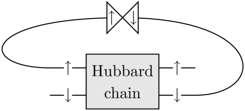
Figure 13: A Hubbard chain is closed to a ring by a single-channel lead attached to different spin channels. Within the embedding method, one therefore has to introduce a spin-flip in the noninteracting lead.

The absence of spin-flip transmissions (31) can be confirmed using the formalism presented in Section 5. Four of the six possible single-channel configurations connect channels of different spin orientation. The spin has then to be flipped somewhere in the noninteracting lead as is indicated in Figure 13 for one of these configurations. The contribution of the kinetic energy to the total Hamiltonian (27) in this example reads

$$H_{\mathrm{K}}=-\Bigg{[}\sum_{i=-L/2}^{L_{\mathrm{S}}-1}c_{i,\uparrow}^{\dagger}c_{i+1,\uparrow}^{\phantom{\dagger}} +\sum_{i=1}^{L/2-1}c_{i,\downarrow}^{\dagger}c_{i+1,\downarrow}^{\phantom{\dagger}}$$ (52)

$$+c_{-L/2,\uparrow}^{\dagger}c_{L/2,\downarrow}^{\phantom{\dagger}}+\text{h.c.}\Bigg{]}\,,$$

where the third term on the right-hand side is responsible for the spin flip.

In a single-channel configuration linking different spin channels, no persistent current can occur. A non-vanishing persistent current in the presence of a spin flip term would result in an accumulation of one spin orientation in the ring. In a stationary situation, this is of course impossible.

It can be seen from the relations presented in Appendix C between the persistent currents in different single-channel rings and the effective transmission amplitudes that the vanishing of persistent currents in setups connecting different spin channels is consistent with the vanishing of the transmission amplitudes with spin flip (31).

Appendix C Reduction of a two-channel scattering problem to effective one-channel scattering problems

As illustrated in Figure 12 for two channels, the effective one-channel scattering problem is obtained by closing on themselves one pair of channels and connecting the remaining pair by a non-interacting lead. The closing of a channel allows in (9) to make the corresponding in- and outgoing amplitudes equal, thus reducing by two the number of amplitudes involved in the scattering problem.

The closing of a channel implies that the amplitudes of the corresponding in- and outgoing channels become equal. Therefore, the closing of two channels reduces the number of amplitudes appearing in (9) from 8 to 6. Furthermore, we can use two of these equations in order to eliminate the remaining two amplitudes related with the closed channels. This leaves us with two equations relating the amplitudes of the open channels and thus defining the effective one-channel problem.

This procedure results in a transfer matrix of considerable complexity when expressed in terms of the parameters of the full scattering problem. The complexity also becomes apparent when one expresses the transfer matrix in terms of the transmission and reflection coefficients as well as the phases encountered on all internal scattering sequences leading from one open channel to the other.

Two different kinds of one-channel setups must be distinguished, depending on whether they connect channels on opposite sides or on the same side. For the first group the moduli of the transmission amplitudes are

$$T_{12} =Q_{1}(\gamma,\theta,\beta,\eta,\varphi,\psi)$$ (53)

$$T_{34} =Q_{1}(\alpha,\epsilon,\beta,\eta,\varphi-\pi/2,\psi-\pi/2)$$

$$T_{13} =Q_{1}(\gamma,\epsilon,\beta,\eta,\varphi,\psi-\pi/2)$$

$$T_{24} =Q_{1}(\alpha,\theta,\beta,\eta,\varphi-\pi/2,\psi)\,,$$

where

$$Q_{1}(\omega_{1},\omega_{2},\omega_{3},\omega_{4},\omega_{5},\omega_{6})=\\ 2\sqrt{\frac{N_{1}(\omega_{1},\omega_{2},\omega_{3},\omega_{4},\omega_{5},\omega_{6})^{2}}{D_{1}(\omega_{1},\omega_{2},\omega_{3},\omega_{4},\omega_{5},\omega_{6})}}\,,$$ (54)

while for the second group we have

$$T_{14} =Q_{2}(\varphi,\psi,\epsilon,\theta,\eta,\beta)$$ (55)

$$T_{23} =Q_{2}(\psi,\varphi,\alpha,\gamma,\beta,\eta)$$

with

$$Q_{2}(\omega_{1},\omega_{2},\omega_{3},\omega_{4},\omega_{5},\omega_{6})=\\ 2\sqrt{\frac{N_{2}(\omega_{1},\omega_{2},\omega_{3},\omega_{4},\omega_{5},\omega_{6})^{2}}{D_{2}(\omega_{2},\omega_{3},\omega_{5},\omega_{4})}}\,.$$ (56)

The fact that each of the two groups is characterized by a single function, $Q_{1}$ or $Q_{2}$, stems from the symmetries of the problem.

In (54), we have introduced the definitions

$$N_{1}(\omega_{1},\omega_{2},\omega_{3},\omega_{4},\omega_{5},\omega_{6}) =$$ (57)

$$t_{1}\cos(\omega_{5})\cos(\omega_{6})[ r_{2}\cos(\omega_{1}+\omega_{3}-\omega_{2}-\omega_{4})$$

$$-\cos(\omega_{1}+\omega_{3}+\omega_{2}+\omega_{4})]$$

$$-t_{2}\sin(\omega_{5})\sin(\omega_{6})[ r_{1}\cos(\omega_{1}-\omega_{2})$$

$$-\cos(\omega_{1}+\omega_{2})]$$

and

$$D_{1}(\omega_{1},\omega_{2},\omega_{3},\omega_{4},\omega_{5},\omega_{6})=\\ [H_{1}^{\text{c}}(\omega_{1},\omega_{2},\omega_{3},\omega_{4},\omega_{5},\omega_{6})-1]^{2}\\ +H_{1}^{\text{s}}(\omega_{1},\omega_{2},\omega_{3},\omega_{4},\omega_{5},\omega_{6})^{2}$$ (58)

where

$$H_{1}^{i}(\omega_{1},\omega_{2}, \omega_{3},\omega_{4},\omega_{5},\omega_{6})=$$ (59)

$$r_{1} A_{2}^{i}(\omega_{1},\omega_{2},\omega_{5}-\pi/2,\omega_{6}-\pi/2)$$

$$+r_{2} A_{2}^{i}(\omega_{1}+\omega_{3},\omega_{2}+\omega_{4},\omega_{5},\omega_{6})$$

$$-r_{1}r_{2} A_{3}^{i}(\omega_{1}+\omega_{2}+\omega_{3},\omega_{1}+\omega_{2}+\omega_{4},\omega_{5},\omega_{6}-\pi/2)$$

$$+ A_{1}^{i}(\omega_{1}+\omega_{2},\omega_{3}+\omega_{4},\omega_{5}-\pi/2,\omega_{6}-\pi/2)$$

$$- A_{3}^{i}(\omega_{1}+\omega_{2}+\omega_{3}+\omega_{4},\omega_{1}+\omega_{2},\omega_{5},\omega_{6})\,,$$

with $i=\text{c},\text{s}$ and

$$A_{1}^{\text{c}}(\omega_{1},\omega_{2},\omega_{3},\omega_{4})=$$ (60)

$$2t_{1}t_{2}\cos(\omega_{3}) \cos(\omega_{4})\sin(\omega_{3})\sin(\omega_{4})\cos(2\omega_{1}+\omega_{2})$$

$$A_{1}^{\text{s}}(\omega_{1},\omega_{2},\omega_{3},\omega_{4})=$$

$$2t_{1}t_{2}\cos(\omega_{3}) \cos(\omega_{4})\sin(\omega_{3})\sin(\omega_{4})\sin(2\omega_{1}+\omega_{2})$$

$$A_{2}^{\text{c}}(\omega_{1},\omega_{2},\omega_{3},\omega_{4})= \cos(\omega_{3})^{2}\cos(2\omega_{1})$$

$$+\cos(\omega_{4})^{2}\cos(2\omega_{2})$$

$$A_{2}^{\text{s}}(\omega_{1},\omega_{2},\omega_{3},\omega_{4})= \cos(\omega_{3})^{2}\sin(2\omega_{1})$$

$$+\cos(\omega_{4})^{2}\sin(2\omega_{2})$$

$$A_{3}^{\text{c}}(\omega_{1},\omega_{2},\omega_{3},\omega_{4})= \cos(\omega_{3})^{2}\cos(\omega_{4})^{2}\cos(2\omega_{1})$$

$$+\sin(\omega_{3})^{2}\sin(\omega_{4})^{2}\cos(2\omega_{2})$$

$$A_{3}^{\text{s}}(\omega_{1},\omega_{2},\omega_{3},\omega_{4})= \cos(\omega_{3})^{2}\cos(\omega_{4})^{2}\sin(2\omega_{1})$$

$$+\sin(\omega_{3})^{2}\sin(\omega_{4})^{2}\sin(2\omega_{2})\,.$$

The functions appearing in $Q_{2}$ are defined as

$$N_{2}(\omega_{1},\omega_{2},\omega_{3},\omega_{4},\omega_{5},\omega_{6}) =$$ (61)

$$t_{1}t_{2}\cos(2\omega_{1})\sin(2\omega_{2}) \sin(\omega_{3}-\omega_{4})$$

$$-\sin(2\omega_{1})\big{(}\sin(\omega_{2})^{2} \sin(\omega_{3}-\omega_{4}+\omega_{5}+\omega_{6})$$

$$-\cos(\omega_{2})^{2} \sin(\omega_{3}-\omega_{4}-\omega_{5}-\omega_{6})$$

$$-r_{2} \sin(\omega_{3}+\omega_{4}+\omega_{5}-\omega_{6})$$

$$+r_{1} \sin(\omega_{3}+\omega_{4}+\omega_{5}+\omega_{6})$$

$$-r_{1}r_{2}[\cos(\omega_{2})^{2} \sin(\omega_{3}-\omega_{4}-\omega_{5}+\omega_{6})$$

$$-\sin(\omega_{2})^{2} \sin(\omega_{3}-\omega_{4}+\omega_{5}-\omega_{6})]\big{)}\,,$$

$$D_{2}(\omega_{2},\omega_{3},\omega_{5},\omega_{4}) =[H_{2}^{\text{c}}(\omega_{2},\omega_{3},\omega_{5},\omega_{4})-1]^{2}$$ (62)

$$\quad+H_{2}^{\text{s}}(\omega_{2},\omega_{3},\omega_{5},\omega_{4})^{2}\,,$$

$$H_{2}^{\text{c}}(\omega_{2},\omega_{3},\omega_{5},\omega_{4}) =r_{1}A_{4}^{\text{c}}(\omega_{2},\omega_{3},\omega_{4})$$ (63)

$$\quad+r_{2}A_{4}^{\text{c}}(\omega_{2},\omega_{2}+\omega_{4},\omega_{1}+\omega_{5})$$

$$\quad-r_{1}r_{2}\cos[2(\omega_{3}+\omega_{5}+\omega_{4})]$$

$$H_{2}^{\text{s}}(\omega_{2},\omega_{3},\omega_{5},\omega_{4}) =r_{1}A_{4}^{\text{s}}(\omega_{2},\omega_{3},\omega_{4})$$

$$\quad+r_{2}A_{4}^{\text{s}}(\omega_{2},\omega_{2}+\omega_{4},\omega_{1}+\omega_{5})$$

$$\quad-r_{1}r_{2}\sin[2(\omega_{3}+\omega_{5}+\omega_{4})]\,,$$

and

$$A_{4}^{\text{c}}(\omega_{2},\omega_{3},\omega_{4}) =\cos(\omega_{2})^{2}\cos(2\omega_{3})+\sin(\omega_{2})^{2}\cos(2\omega_{4})$$ (64)

$$A_{4}^{\text{s}}(\omega_{2},\omega_{3},\omega_{4}) =\cos(\omega_{2})^{2}\sin(2\omega_{3})+\sin(\omega_{2})^{2}\sin(2\omega_{4})\,.$$

References

- (1) D. Goldhaber-Gordon, H. Shtrikman, D. Mahalu, D. Abusch-Magder, U. Meirav, M.A. Kastner, Nature 391, 156 (1998)
- (2) M. Pustilnik, L.I. Glazman, D.H. Cobden, L.P. Kouwenhoven, Lect. Notes Phys. 579, 3 (2001)
- (3) A.C. Hewson, The Kondo Problem to Heavy Fermions (Cambridge University Press, Cambridge, 1997)
- (4) P. Mehta, N. Andrei, Phys. Rev. Lett. 96, 216802 (2006); Erratum: P. Mehta, S.-P. Chao, N. Andrei, e-print arXiv:cond-mat/0703426v1
- (5) B. Doyon, Phys. Rev. Lett. 99, 076806 (2007)
- (6) E. Boulat, H. Saleur, P. Schmitteckert, Phys. Rev. Lett. 101, 140601 (2008)
- (7) P. Schmitteckert, F. Evers, Phys. Rev. Lett. 100, 086401 (2008)
- (8) Y. Meir, N.S. Wingreen, Phys. Rev. Lett. 68, 2512 (1992)
- (9) J. Favand, F. Mila, Eur. Phys. J. B 2, 293 (1998)
- (10) O.P. Sushkov, Phys. Rev. B 64, 155319 (2001)
- (11) R.A. Molina, D. Weinmann, R.A. Jalabert, G.-L. Ingold, J.-L. Pichard, Phys. Rev. B 67, 235306 (2003)
- (12) V. Meden, U. Schollwöck, Phys. Rev. B 67, 193303 (2003)
- (13) T. Rejec, A. Ramšak, Phys. Rev. B 68, 035342 (2003)
- (14) R.A. Molina, P. Schmitteckert, D. Weinmann, R.A. Jalabert, G.-L. Ingold, J.-L. Pichard, Eur. Phys. J. B 39, 107 (2004)
- (15) R.A. Molina, D. Weinmann, J.-L. Pichard, Eur. Phys. J. B 48, 243 (2005)
- (16) A.O. Gogolin, N.V. Prokof’ev, Phys. Rev. B 50, 4921 (1994)
- (17) D. Weinmann, R.A. Jalabert, A. Freyn, G.-L. Ingold, J.-L. Pichard, Eur. Phys. J. B 66, 239 (2008)
- (18) G. Vasseur, Ph.D. thesis, Université Louis Pasteur Strasbourg, 2006, e-print http://eprints-scd-ulp.u-strasbg.fr:8080/574/
- (19) P.A. Mello, J.-L. Pichard, J. Phys. I 1, 493 (1991)
- (20) C.W.J. Beenakker, Rev. Mod. Phys. 69, 731 (1997)
- (21) R.A. Jalabert, J.-L. Pichard, J. Phys. I 5, 287 (1995)
- (22) X. Waintal, G. Fleury, K. Kazymyrenko, M. Houzet, P. Schmitteckert, D. Weinmann, Phys. Rev. Lett. 101, 106804 (2008)
- (23) S.R. White, Phys. Rev. Lett. 69, 2863 (1992)
- (24) Density-Matrix Renormalization — A New Numerical Method in Physics, edited by I. Peschel, X. Wang, M. Kaulke, K. Hallberg, Lect. Notes Phys. 528, 1–355 (Springer, Berlin, 1999)
- (25) P. Schmitteckert, Ph.D. thesis, Universität Augsburg, 1996
- (26) A. Oguri, Phys. Rev. B 63, 115305 (2001)
- (27) Y. Nisikawa, A. Oguri, Phys. Rev. B 73, 125108 (2006)
- (28) A. Oguri, Phys. Rev. B 59, 12240 (1999)
- (29) A. Oguri, A.C. Hewson, J. Phys. Soc. Jpn. 74, 988 (2005)
- (30) P. Schmitteckert, R. Werner, Phys. Rev. B 69, 195115 (2004)
- (31) D. Bohr, P. Schmitteckert, P. Wölfle, Europhys. Lett. 73, 246 (2006)
- (32) T.K. N’g, P.A. Lee, Phys. Rev. Lett. 61, 1768 (1988)
- (33) A. Freyn, J.-L. Pichard, e-print arXiv:0904.0889v1