Deriving SN from PSN: a general proof technique

Abstract

In the framework of explicit substitutions there is two termination properties: preservation of strong normalization (PSN), and strong normalization (SN). Since there are not easily proved, only one of them is usually established (and sometimes none). We propose here a connection between them which helps to get SN when one already has PSN. For this purpose, we formalize a general proof technique of SN which consists in expanding substitutions into “pure” $\lambda$-terms and to inherit SN of the whole calculus by SN of the “pure” calculus and by PSN. We apply it successfully to a large set of calculi with explicit substitutions, allowing us to establish SN, or, at least, to trace back the failure of SN to that of PSN.

1 Introduction

Calculi with explicit substitutions were introduced [1] as a bridge between $\lambda$-calculus [7, 2] and concrete implementations of functional programming languages. Those calculi intend to refine the evaluation process by proposing reduction rules to deal with the substitution mechanism – a meta-operation in the traditional $\lambda$-calculus. It appears that, with those new rules, it was much harder (and sometimes impossible) to get termination properties.

The two main termination properties of calculi with explicit substitutions are:

• Preservation of strong normalization (PSN), which says that if a pure term (i.e. without explicit substitutions) is strongly normalizing (i.e. cannot be infinitely reduced) in the pure calculus (i.e. the calculus without explicit substitutions), then this term is also strongly normalizing with respect to the calculus with explicit substitutions.

• Strong normalization (SN), which says that, with respect to a typing system, every typed term is strongly normalizing in the calculus with explicit substitutions, i.e. every terms in the subset of typed terms cannot be infinitely reduced.

These two properties are not redundant, and Fig. 1 shows the differences between them. PSN says that the horizontally and diagonally hatched rectangle is included in the diagonally hatched rectangle. SN says that the vertically hatched rectangle is included in the diagonally hatched rectangle. Even if they work on a different set of terms, there is a common part: the vertically and horizontally hatched rectangle, which represent the typed pure terms.

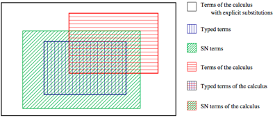
Figure 1: Termination properties

SN and PSN are both termination properties, although their proofs are not always clearly related: sometimes SN is shown independently of PSN (directly, by simulation, etc., see for example [8, 10]), sometimes SN proofs uses PSN (see for example [4]). We present here a general proof technique of SN via PSN, initially suggested by H. Herbelin, which uses that common part of typed pure terms.

More formally, we may introduce the following notations: we denote $\Lambda$ the set of $\lambda$-terms, $\Lambda_{T}$ the set of typed $\Lambda$-terms with a given typing system $T$, $\Lambda_{SN}$ the set of terminating $\Lambda$-terms (i.e. with a finite derivation tree); we denote $\Lambda^{X}$, $\Lambda^{X}_{T}$, $\Lambda^{X}_{SN}$ the corresponding set for calculi with eXplicit substitutions.

By definition, we have the following set inclusions:

$$\Lambda_{T}\subset\Lambda\;\;\;\;\mbox{and}\;\;\;\;\Lambda_{SN}\subset\Lambda$$

$$\Lambda^{X}_{T}\subset\Lambda^{X}\;\;\;\;\mbox{and}\;\;\;\;\Lambda^{X}_{SN}\subset\Lambda^{X}$$

$$\Lambda\subset\Lambda^{X}\;\;\;\;\mbox{and}\;\;\;\;\Lambda_{T}\subset\Lambda^{X}_{T}$$

The usual strong normalisation property of typed $\lambda$-calculus gives

$$\Lambda_{T}\subset\Lambda_{SN}$$

As regard to calculi with explicit substitutions, we have the following properties. At first, the property PSN gives

$$\Lambda_{SN}\subset\Lambda^{X}_{SN}$$

At last, the strong normalization property of typed $\Lambda^{X}$-terms completes with the following inclusion:

$$\Lambda^{X}_{T}\subset\Lambda^{X}_{SN}$$

In the following section, we formalize a proof technique that exploits this diagram and in the remaining sections we apply this technique to a set of calculi. This set has been chosen for the variety of their definitions: with or without De Bruijn indices, unary or multiple substitutions, with or without composition of substitutions, and even a symmetric non-deterministic calculus. In the last section, we briefly talk about perspectives in this framework.

2 Proof Technique

The idea of this technique is the following. Let $t$ be a typed term with explicit substitutions for which we want to show termination. With the help of its typing judgment, we build a typed pure term $t^{\prime}$ which can be reduced to $t$. For that purpose, we expand the substitutions of $t$ into redexes. We call this expansion $\mathit{Ateb}$ (the opposite of $\mathit{Beta}$ which is usually the name of the rule which creates explicit substitutions). Then, with SN of the pure calculus and PSN, we can export the strong normalization of $t^{\prime}$ (in the pure calculus) to $t$ (in the calculus with explicit substitutions).

In practice, this sketch will only apply in some cases, and some others will require some adjustment to this technique. For our technique to work, we need that the $\mathit{Ateb}$ expansion satisfies some properties. The first one is always easily checked.

Property 2.1 (Preservation of typability)

If $t$ is typable, with respect to a typing system $T$, in the calculus with explicit substitution, then $\mathit{Ateb}(t)$ is typable, with respect to a typing system $T^{\prime}$ (possibly $T^{\prime}=T$) in the pure calculus.

Only some calculi can exhibit an $\mathit{Ateb}$ function which satisfies the second one.

Property 2.2 (Initialization)

$\mathit{Ateb}(t)$ reduces to $t$ in zero or more steps in the calculus with explicit substitutions.

If we can get it, then we use the direct proof to be presented in section 2.1. Otherwise, we need to use the simulation proof to be presented in section 2.2.

2.1 Direct proof

We can immediately establish the theorem.

Theorem 2.3

For all typing systems $T$ and $T^{\prime}$ such that, in the pure calculus, all typable terms with respect to $T$ are strongly normalizing, if there exists a function $\mathit{Ateb}$ from explicit substitution terms to pure terms satisfying properties 2.1 and 2.2 then PSN implies SN (with respect to $T^{\prime}$).

Proof.

For every typed term $t$ of the calculus with explicit substitution, $\mathit{Ateb}(t)$ is a pure typed term (by property 2.1). By the strong normalization hypothesis of the typed pure calculus, we have $\mathit{Ateb}(t)\in\Lambda_{SN}$. By hypothesis of PSN we obtain that $\mathit{Ateb}(t)$ is in $\Lambda^{X}_{SN}$. By property 2.2, we get $\mathit{Ateb}(t)\rightarrow^{*}t$, which gives us directly $t\in\Lambda^{X}_{SN}$. ∎

2.2 Simulation proof

We must relax some constraints on $\mathit{Ateb}$. We will try to find an expansion of $t$ to $t^{\prime}$ such that $t^{\prime}$ reduces to a term $u$ and there exists a relation $\mathcal{R}$ with $u\mathcal{R}t$. The chosen relation must, in addition, enable a simulation of the reductions of $t$ by the reduction of $u$. If it is possible, we can infer strong normalization of $t$ from strong normalization of $u$.

To proceed with the simulation, we first split the reduction rules of the calculus with explicit substitutions into two disjoints sets. The set $R_{1}$ contains rules which are trivially terminating, and $R_{2}$ contains the others. Secondly, we build a relation $\mathcal{R}$ which satisfies the following properties.

Property 2.4 (Initialisation)

For every typed term $t$, there exists a term $u\mathcal{R}t$ such that $\mathit{Ateb}(t)$ reduces in 0 or more steps to $u$ in the calculus with explicit substitutions.

Property 2.5 (Simulation ^∗)

For every term $t$, if $t\rightarrow_{R_{1}}t^{\prime}$ then, for every $u\mathcal{R}t$, there exists $u^{\prime}$ such that $u\rightarrow^{*}u^{\prime}$ and $u^{\prime}\mathcal{R}t^{\prime}$.

Property 2.6 (Simulation ⁺)

For every term $t$, if $t\rightarrow_{R_{2}}t^{\prime}$ then, for every $u\mathcal{R}t$, there exists $u^{\prime}$ such that $u\rightarrow^{+}u^{\prime}$ and $u^{\prime}\mathcal{R}t^{\prime}$.

We display those properties as diagrams :

$$\begin{array}[]{r@{\ }l@{\ }c}\lx@intercol\hfil\mbox{Initialisation}\hfil\lx@intercol\\ \\ &&t\\ &\swarrow&\mathcal{R}\\ \mathit{Ateb}(t)&\rightarrow^{*}&u\end{array}\hskip 56.9055pt\begin{array}[]{ccc}\lx@intercol\hfil\mbox{Simulation ${}^{*}$}\hfil\lx@intercol\\ \\ t&\;\;\rightarrow_{R_{1}}&t^{\prime}\\ \mathcal{R}&&\mathcal{R}\\ u&\rightarrow^{*}&u^{\prime}\end{array}\hskip 56.9055pt\begin{array}[]{ccc}\lx@intercol\hfil\mbox{Simulation ${}^{+}$}\hfil\lx@intercol\\ \\ t&\;\;\rightarrow_{R_{2}}&t^{\prime}\\ \mathcal{R}&&\mathcal{R}\\ u&\rightarrow^{+}&u^{\prime}\end{array}$$

With this material, we can establish the theorem.

Theorem 2.7

For all typing systems $T$ and $T^{\prime}$ such that, in the pure calculus, all typable terms with respect to $T$ are strongly normalizing, if there exists a function $\mathit{Ateb}$ from explicit substitution terms to pure terms and a relation $\mathcal{R}$ on explicit substitutions terms satisfying properties 2.1, 2.4, 2.5 and 2.6 then PSN implies SN (with respect to $T^{\prime}$).

Proof.

We prove it by contradiction. Let $t$ be a typed term with explicit substitutions which can be infinitely reduced. By property 2.4 there exists a term $u$ such that $\mathit{Ateb}(t)\rightarrow^{*}u$, and $\mathit{Ateb}(t)$ is a pure typed term (by property 2.1). By the strong normalization hypothesis of the typed pure calculus, we have $\mathit{Ateb}(t)\in\Lambda_{SN}$. By hypothesis of PSN we obtain that $\mathit{Ateb}(t)$ is in $\Lambda^{X}_{SN}$ and it follows that $u\in\Lambda^{X}_{SN}$.

By property 2.4, we also have $u\mathcal{R}t$, and, with properties 2.5 and 2.6, we can build an infinite reduction from $u$, contradicting the strong normalization of $u$. ∎

3 $\lambda{\tt x}$-calculus

The $\lambda{\tt x}$-calculus [6, 5] is probably the simplest calculus with explicit substitutions. It only makes the substitution explicit. Since this calculus provides no rules to deal with substitutions composition, it preserves strong normalization. It is for this calculus that the technique has been originate used by Herbelin. Therefore, we can without surprises apply the direct proof to get strong normalization.

3.1 Definition

Terms of the $\lambda{\tt x}$-calculus are given by the following grammar:

$$t::=x\ |\ (t\ t)\ |\ \lambda x.t\ |\ t[t/x]$$

Here follows the reduction rules:

$$\begin{array}[]{rcl}(\lambda x.t)u&\rightarrow_{\mathit{Beta}}&t[u/x]\\ (t\ u)[v/x]&\rightarrow_{\mathit{App}}&(t[v/x])\ (u[v/x])\\ (\lambda x.t)[u/y]&\rightarrow_{\mathit{Lambda}}&\lambda x.(t[u/y])\\ x[t/x]&\rightarrow_{\mathit{Var1}}&t\\ y[t/x]&\rightarrow_{\mathit{Var2}}&y\\ \end{array}$$

The rule $\mathit{Lambda}$ is applied modulo $\alpha$-conversion of the bound variable $x$.

Here follows the typing rules:

$\Gamma,x:A\vdash x:A$	$\Gamma\vdash t[u/x]:A\lx@proof@logical@and\Gamma\vdash u:B\Gamma,x:B\vdash t:A$
$\Gamma\vdash(t\ u):A\lx@proof@logical@and\Gamma\vdash t:B\rightarrow A\Gamma\vdash u:B$	$\Gamma\vdash\lambda x.t:B\rightarrow A\Gamma,x:B\vdash t:A$

3.2 Strong normalisation proof

We define the $\mathit{Ateb}$ function as follows:

$\mathit{Ateb}(x)$	$=$	$x$
$\mathit{Ateb}(t\ u)$	$=$	$\mathit{Ateb}(t)\ \mathit{Ateb}(u)$
$\mathit{Ateb}(\lambda x.t)$	$=$	$\lambda x.\mathit{Ateb}(t)$
$\mathit{Ateb}(t[u/x])$	$=$	$(\lambda x.\mathit{Ateb}(t))\ \mathit{Ateb}(u)$

Remark that $\mathit{Ateb}$ performs the exact reverse rewriting of the rule $\mathit{Beta}$. It straightforwardly follows that if $t^{\prime}=\mathit{Ateb}(t)$ then $t^{\prime}\rightarrow_{\mathit{Beta}}^{*}t$ and $\mathit{Ateb}(t)$ does not contain any substitutions.

We check that the $\mathit{Ateb}(t)$ is typable.

Lemma 3.1

$$\Gamma\vdash t:A\;\;\Rightarrow\;\;\Gamma\vdash\mathit{Ateb}(t):A$$

Proof.

By induction on the typing derivation of $t$. The only non-trivial case is that of substitutions. We have $t=u[v/x]$ and

$$\Gamma\vdash u[v/x]:A\lx@proof@logical@and\Gamma\vdash v:B\Gamma,x:B\vdash u:A$$

By induction hypothesis, we have $\Gamma,x:B\vdash\mathit{Ateb}(u):A$ and $\Gamma\vdash\mathit{Ateb}(v):B$. We can build the typing derivation of $\mathit{Ateb}(t)=\lambda x.\mathit{Ateb}(u))\ \mathit{Ateb}(v)$ as follows

$$\Gamma\vdash(\lambda x.\mathit{Ateb}(u))\ \mathit{Ateb}(v):A\lx@proof@logical@and\Gamma\vdash\lambda x.\mathit{Ateb}(u):B\rightarrow A\Gamma,x:B\vdash\mathit{Ateb}(u):A\Gamma\vdash\mathit{Ateb}(v):B$$

∎

We can apply Theorem 2.3.

Corollary 3.2

Since the $\lambda{\tt x}$-calculus enjoys PSN [6] and the $\lambda$-calculus enjoys SN of simply-typed terms [11], we conclude that the $\lambda{\tt x}$-calculus enjoys SN of simply-typed terms.

4 $\lambda\upsilon$-calculus

The $\lambda\upsilon$-calculus [12, 3] is the De Bruijn counterpart of $\lambda{\tt x}$. As $\lambda{\tt x}$, it has no composition rules, and therefore satisfies PSN. For this calculus, we must use the simulation proof to deal with indices modification operators. We succeed to use it and it is, as far as we know, the first proof of SN for a simply typed version of $\lambda\upsilon$ (see [13]).

4.1 Definition

Terms of $\lambda\upsilon$-calculus are given by the following grammar:

$$\begin{array}[]{l}t::=n\ |\ (t\ t)\ |\ \lambda t\ |\ t[s]\\ s::=a/\ |\ \Uparrow(s)\ |\ \uparrow\\ \end{array}$$

Remark that a substitution is always build from a (possibly empty) list of $\Uparrow$ followed by either a $t/$, or a $\uparrow$. We will then write substitutions in a more general form: either $t[\Uparrow^{i}(t/)]$, or $t[\Uparrow^{i}(\uparrow)]$, where $\Uparrow^{i}(s)$ denotes $\underset{i}{\underbrace{\Uparrow(\Uparrow(...(\Uparrow}}(s))...))$.

Here follows the reduction rules:

$$\begin{array}[]{lll}(\lambda t)u&\rightarrow_{B}&t[u/]\\ (t\ u)[s]&\rightarrow_{\mathit{App}}&(t[s])\ (u[s])\\ (\lambda t)[s]&\rightarrow_{\mathit{Lambda}}&\lambda(t[\Uparrow(s)])\\ 1[t/]&\rightarrow_{\mathit{FVar}}&t\\ n+1[t/]&\rightarrow_{\mathit{RVar}}&n\\ 1[\Uparrow(s)]&\rightarrow_{\mathit{FVarLift}}&1\\ n+1[\Uparrow(s)]&\rightarrow_{\mathit{RVarLift}}&n[s][\uparrow]\\ n[\uparrow]&\rightarrow_{\mathit{VarShift}}&n+1\\ \end{array}$$

Here follows the typing rules (where $n=|\Gamma|+1$) :

$\Gamma,A,\Delta\vdash n:A$	$\Gamma\vdash t[s]:A\lx@proof@logical@and\Gamma\vdash s\triangleright\Gamma^{\prime}\Gamma^{\prime}\vdash t:A$
$\Gamma\vdash(t\ u):A\lx@proof@logical@and\Gamma\vdash t:B\rightarrow A\Gamma\vdash u:B$	$\Gamma\vdash\lambda t:B\rightarrow AB,\Gamma\vdash t:A$

$\Gamma\vdash t/\triangleright A,\Gamma\Gamma\vdash t:A$

$A,\Gamma\vdash\uparrow\triangleright\ \Gamma$

$A,\Gamma\vdash\Uparrow(s)\triangleright A,B,\Gamma\Gamma\vdash s\triangleright B,\Gamma$

4.2 Strong normalisation proof

We define the $\mathit{Ateb}$ function as follows:

$$\begin{array}[]{lll}\mathit{Ateb}(n)&=&n\\ \mathit{Ateb}(t\ u)&=&\mathit{Ateb}(t)\ \mathit{Ateb}(u)\\ \mathit{Ateb}(\lambda t)&=&\lambda\mathit{Ateb}(t)\\ \mathit{Ateb}(t[u/])&=&(\lambda\mathit{Ateb}(t))\ \mathit{Ateb}(u)\\ \mathit{Ateb}(t[\Uparrow^{i}(u/)])&=&(\lambda I_{i}(\mathit{Ateb}(t)))\ K_{i}(\mathit{Ateb}(u))\\ \mathit{Ateb}(t[\Uparrow^{i}(\uparrow)])&=&J_{i}(\mathit{Ateb}(t))\\ \end{array}$$

Example 4.1

For instance, if we suppose that for any $tt$ among $t$, $u$, $v$, $w$ we have $tt=\mathit{Ateb}(tt)$, then we get

$$\mathit{Ateb}((t[u/]\ v[\Uparrow(\Uparrow(\Uparrow(w/)))])[\Uparrow(\Uparrow(\uparrow))])\;\;\;=\;\;\;J_{2}(((\lambda t)u)\ ((\lambda I_{3}(v))K_{3}(w)))$$

Where $I_{i}(t))$, $K_{i}(t)$ and $J_{i}(t)$ are functions that we will define in the sequel. The intuition about those function is the following: substitutions perform some re-indexing of terms upon which they are applied, those functions intend to anticipate this re-indexing. To understand the necessity of those functions, let us look at some typing derivation. To begin with, we take $t[\Uparrow^{i}(u/)]$, where $\Delta=D_{i},...,D_{1}$ ($i=|\Delta|$) :

$$\Delta,\Gamma\vdash t[\Uparrow^{i}(u/)]:A\lx@proof@logical@and D_{i},D_{i-1},...,D_{1},\Gamma\vdash\Uparrow^{i}(u/)\triangleright D_{i},D_{i-1},...,D_{1},B,\Gamma D_{i-1},...,D_{1},\Gamma\vdash\Uparrow^{i-1}(u/)\triangleright D_{i-1},...,D_{1},B,\Gamma\vdots D_{1},\Gamma\vdash\Uparrow(u/)\triangleright D_{1},B,\Gamma\Gamma\vdash u/\triangleright B,\Gamma\Gamma\vdash u:B\Delta,B,\Gamma\vdash t:A$$

We would like to type a term of the form $(\lambda t^{\prime})u^{\prime}$, that is

$$\Delta,\Gamma\vdash(\lambda t^{\prime})u^{\prime}:A\lx@proof@logical@and\Delta,\Gamma\vdash\lambda t^{\prime}:B\rightarrow AB,\Delta,\Gamma\vdash t^{\prime}:A\Delta,\Gamma\vdash u^{\prime}:B$$

The problem is to build a term $t^{\prime}$ from $t$ which would be typeable in the environment $B,\Delta,\Gamma$ instead of $\Delta,B,\Gamma$ and a term $u^{\prime}$ from $u$ which would be typeable in the environment $\Delta,\Gamma$ instead of $\Gamma$. This is exactly the work of the functions $I_{i}(\ )$ and $K_{i}(\ )$ respectively. Look now at the typing derivation of $t[\Uparrow^{i}(\uparrow)]$, where $\Delta=D_{i},...,D_{1}$ ($i=|\Delta|$) :

$$\Delta,B,\Gamma\vdash t[\Uparrow^{i}(\uparrow)]:A\lx@proof@logical@and D_{i},D_{i-1},...,D_{1},B,\Gamma\vdash\Uparrow^{i}(\uparrow)\triangleright D_{i},D_{i-1},...,D_{1},\Gamma D_{i-1},...,D_{1},B,\Gamma\vdash\Uparrow^{i-1}(\uparrow)\triangleright D_{i-1},...,D_{1},\Gamma\vdots D_{1},B,\Gamma\vdash\Uparrow(\uparrow)\triangleright D_{1},\Gamma B,\Gamma\vdash\uparrow\triangleright\Gamma\Delta,\Gamma\vdash t:A$$

The problem here is to build a term $t^{\prime}$ from $t$ which would be typeable in the environment $\Delta,B,\Gamma$ instead of $\Delta,\Gamma$. This is done by the function $J_{i}(\ )$. We can state the property that should verify those functions.

Property 4.2

For any term $t$ we have (with $i=|\Delta|$) :

• $\Gamma\vdash t:A\;\;\;\Rightarrow\;\;\;\Delta,\Gamma\vdash K_{i}(t):A$

• $\Delta,B,\Gamma\vdash t:A\;\;\;\Rightarrow\;\;\;B,\Delta,\Gamma\vdash I_{i}(t):A$

• $\Delta,\Gamma\vdash t:A\;\;\;\Rightarrow\;\;\;\Delta,B,\Gamma\vdash J_{i}(t):A$

We can then check that the term obtained by the function $\mathit{Ateb}$ is typeable.

Lemma 4.3

$$\Gamma\vdash t:A\;\;\Rightarrow\;\;\Gamma\vdash\mathit{Ateb}(t):A$$

Proof.

By induction on the typing derivation of $t$.

• $t=n$ and

  $$\Gamma,A,\Delta\vdash n:A$$

  We then have $\mathit{Ateb}(t)=n$ and the same typing derivation.

• $t=(u\ v)$ and

  $$\Gamma\vdash(u\ v):A\lx@proof@logical@and\Gamma\vdash u:B\rightarrow A\Gamma\vdash v:B$$

  By induction hypothesis, we have $\Gamma\vdash\mathit{Ateb}(u):B\rightarrow A$ and $\Gamma\vdash\mathit{Ateb}(v):B$. We can type $\mathit{Ateb}(t)=\mathit{Ateb}(u)\ \mathit{Ateb}(v)$ as follows

  $$\Gamma\vdash(\mathit{Ateb}(u)\ \mathit{Ateb}(v)):A\lx@proof@logical@and\Gamma\vdash\mathit{Ateb}(u):B\rightarrow A\Gamma\vdash\mathit{Ateb}(v):B$$

• $t=\lambda u$ and

  $$\Gamma\vdash\lambda u:B\rightarrow AB,\Gamma\vdash u:A$$

  By induction hypothesis, we have $\Gamma,x:B\vdash\mathit{Ateb}(u):A$. We can type $\mathit{Ateb}(t)=\lambda\mathit{Ateb}(u)$ as follows

  $$\Gamma\vdash\lambda\mathit{Ateb}(u):AB,\Gamma\vdash\mathit{Ateb}(u):A$$

• Cases for $t=u[\Uparrow^{i}(v/)]$ and $t=u[\Uparrow^{i}(\uparrow)]$ are treated as discussed above, using property 4.2.

∎

Of course, for any $t$, $\mathit{Ateb}(t)$ does not contain any substitutions.

4.2.1 Functions definitions

The function $J_{i}(t)$ performs the re-indexing of $t$ as if a substitution $[\Uparrow^{i}(\uparrow)]$ has been propagated. Since it is applied to terms obtained by the $\mathit{Ateb}$ function, only terms without substitutions are concerned.

Here follows its definition:

$$\begin{array}[]{llll}J_{i}(n)&=&n+1&\mbox{if }n>i\\ J_{i}(n)&=&n&\mbox{if }n\leq i\\ J_{i}(t\ u)&=&J_{i}(t)\ J_{i}(u)&\\ J_{i}(\lambda t)&=&\lambda J_{i+1}(t)&\\ \end{array}$$

The function $K_{i}(t)$ performs the re-indexing of $t$ as if $i$ substitutions $[\uparrow]$ have been propagated. We can define it from with the help of the function $J_{i}(t)$ :

$$K_{i}(t)=\underset{i}{\underbrace{J_{0}(J_{0}(...J_{0}(t)))}}$$

When this function is applied to a variable, we obtain $K_{i}(n)=n+i$.

The function $I_{i}(t)$ prepares a term $t$ to be applied to a substitution that has lost its $\Uparrow$. It deals also with substitution-free terms.

Here follows its definition:

$$\begin{array}[]{llll}I_{i}(n)&=&n&\mbox{si }n>i+1\\ I_{i}(n)&=&1&\mbox{si }n=i+1\\ I_{i}(n)&=&n+1&\mbox{si }n\leq i\\ I_{i}(t\ u)&=&I_{i}(t)\ I_{i}(u)&\\ I_{i}(\lambda t)&=&\lambda I_{i+1}(t)&\\ \end{array}$$

Indices are transformed as follows: since we have deleted $i$ $\Uparrow$, the index $i+1$ must become $1$. To reflect this change, every index $j$ smaller than $i+1$ must become $j+1$. The others are let unchanged.

Here follows several useful properties.

Property 4.4

For all $t$, $u$, $i$, $j$, We have

$$K_{i}(t)=K_{j}(u)\;\;\;\;\;\Rightarrow\;\;\;\;\;K_{i+1}(t)=K_{j+1}(u)$$

Proof.

Indeed,

$$K_{i}(t)=K_{j}(u)\;\;\;\;\;\Rightarrow\;\;\;\;\;J_{0}(K_{i}(t))=J_{0}(K_{j}(u))$$

∎

Property 4.5

For all $n$ and $i$, we have

$$J_{i+1}(n)\;\;\;\;\;=\;\;\;\;\;K_{1}(J_{i}(n-1))$$

Proof.

We calculate the values accordingly to $n$ and $i$.

• if $n>i+1$ then $J_{i+1}(n)=n$, $J_{i}(n-1)=n-1$ and $K_{1}(n-1)=n$.

• if $n\leq i+1$ then $J_{i+1}(n)=n+1$, $J_{i}(n-1)=n$ and $K_{1}(n)=n+1$.

∎

Property 4.6

For all $n>1$ and $i$, we have

$$I_{i+1}(n)\;\;\;\;\;=\;\;\;\;\;J_{1}(I_{i}(n-1))$$

Proof.

We calculate the values accordingly to $n$ and $i$.

• if $n>i+2$ then $I_{i+1}(n)=n$, $I_{i}(n-1)=n-1$ and $J_{1}(n-1)=n$.

• if $n=i+2$ then $I_{i+1}(n)=1$, $I_{i}(n-1)=1$ and $J_{1}(1)=1$.

• if $n<i+2$ then $I_{i+1}(n)=n+1$, $I_{i}(n-1)=n$ and $J_{1}(n)=n+1$.

∎

Example 4.7

We apply those function to our example, and we obtain

$$J_{2}(((\lambda t)u)\ ((\lambda I_{3}(v))K_{3}(w)))\;\;\;=\;\;\;((\lambda J_{3}(t))J_{2}(u)){\ }((\lambda J_{3}(I_{3}(v)))J_{2}(K_{3}(w)))$$

We can now prove Property 4.2.

Proof.

• $\Delta,\Gamma\vdash t:A\;\;\;\Rightarrow\;\;\;\Delta,B,\Gamma\vdash J_{i}(t):A$. By induction on $t$.

  • $t=n$ with $n\leq i$: $J_{i}(t)=n$. We have

    $$\Delta_{1},A,\Delta_{2},\Gamma\vdash n:A$$

    with $n=|\Delta_{1}|+1$. We conclude with the following typing derivation

    $$\Delta_{1},A,\Delta_{2},B,\Gamma\vdash n:A$$

  • $t=n$ with $n>i$: $J_{i}(t)=n+1$. We have

    $$\Delta,\Gamma_{1},A,\Gamma_{2}\vdash n:A$$

    With $n=|\Delta|+|\Gamma_{1}|+1$. We the get $n+1=|\Delta|+|\Gamma_{1}|+1+1$ and

    $$\Delta,B,\Gamma_{1},A,\Gamma_{2}\vdash n:A$$

  • $t=(u\ v)$: $J_{i}(t)=(J_{i}(u)\ J_{i}(v))$ and we conclude by applying twice the induction hypothesis.

  • $t=\lambda u$ (with $A=C\rightarrow D$) : $J_{i}(t)=\lambda J_{i+1}(u)$. We have

    $$\Delta,\Gamma\vdash\lambda u:C\rightarrow DC,\Delta,\Gamma\vdash u:D$$

    By induction hypothesis, we have $C,\Delta,B,\Gamma\vdash J_{i+1}(u):D$ and we can build the following typing derivation

    $$\Delta,B,\Gamma\vdash\lambda J_{i+1}(u):C\rightarrow DC,\Delta,B,\Gamma\vdash J_{i+1}(u):D$$

• $\Gamma\vdash t:A\;\;\;\Rightarrow\;\;\;\Delta,\Gamma\vdash K_{i}(t):A$. By induction hypothesis on $t$.

  • $t=n$: $K_{i}(n)=\underset{i}{\underbrace{J_{0}(J_{0}(...J_{0}(n)))}}=n+i$. We have

    $$\Gamma_{1},A,\Gamma_{2}\vdash n:A$$

    with $n=|\Gamma_{1}|+1$. Since $i=|\Delta|$, we get $n+i=|\Gamma_{1}|+|\Delta|+1$ and

    $$\Delta,\Gamma_{1},A,\Gamma_{2}\vdash n+i:A$$

  • $t=(u\ v)$: $K_{i}(t)=(K_{i}(u)\ K_{i}(v))$ and we conclude by applying twice the induction hypothesis.

  • $t=\lambda u$ (with $A=C\rightarrow D$): $K_{i}(t)=\underset{i}{\underbrace{J_{0}(J_{0}(...J_{0}(\lambda u)))}}=\lambda\underset{i}{\underbrace{J_{1}(J_{1}(...J_{1}(u)))}}$.

    We get

    $$\Gamma\vdash\lambda u:C\rightarrow DC,\Gamma\vdash u:D$$

    By the item above, we have

    $$\begin{array}[]{c}C,\Gamma\vdash u:D\\ \Downarrow\\ C,E_{1},\Gamma\vdash J_{1}(u):D\\ \Downarrow\\ C,E_{2},E_{1},\Gamma\vdash J_{1}(J_{1}(u)):D\\ \Downarrow\\ \vdots\\ \Downarrow\\ C,E_{i},...,E_{1},\Gamma\vdash\underset{i}{\underbrace{J_{1}(J_{1}(...J_{1}(u)))}}\\ \end{array}$$

    with $\Delta=E_{i},...,E_{1}$. We can then build the following typing derivation

    $$\Delta,\Gamma\vdash K_{i}(\lambda u):C\rightarrow DC,\Delta,\Gamma\vdash\underset{i}{\underbrace{J_{1}(J_{1}(...J_{1}(u)))}}:D$$

• $\Delta,B,\Gamma\vdash t:A\;\;\;\Rightarrow\;\;\;B,\Delta,\Gamma\vdash I_{i}(t):A$. By induction on $t$.

  • $t=n$ with $n>i+1$: $I_{i}(t)=n$. We have

    $$\Delta,B,\Gamma_{1},A,\Gamma_{2}\vdash n:A$$

    with $n=|\Delta|+1+|\Gamma_{1}|+1$. We conclude with the following typing derivation

    $$B,\Delta,\Gamma_{1},A,\Gamma_{2}\vdash n:A$$

  • $t=n$ with $n=i+1$: $I_{i}(t)=1$. We have

    $$\Delta,B,\Gamma\vdash n:B$$

    with $n=i+1=|\Delta|+1$. We conclude with the following typing derivation

    $$B,\Delta,\Gamma\vdash 1:A$$

  • $t=n$ with $n\leq i$: $I_{i}(t)=n+1$. We have

    $$\Delta_{1},A,\Delta_{2},B,\Gamma\vdash n:A$$

    with $n=|\Delta_{1}|+1$. We then get $n+1=|\Delta_{1}|+1+1$ and

    $$B,\Delta_{1},A,\Delta_{2},\Gamma\vdash n:A$$

  • $t=(u\ v)$ : $I_{i}(t)=(I_{i}(u)\ I_{i}(v))$ and we conclude by applying twice the induction hypothesis.

  • $t=\lambda u$ (with $A=C\rightarrow D$) : $I_{i}(t)=\lambda I_{i+1}(u)$. We have

    $$\Delta,B,\Gamma\vdash\lambda u:C\rightarrow DC,\Delta,B,\Gamma\vdash u:D$$

    By induction hypothesis, we have $C,\Delta,\Gamma\vdash I_{i+1}(u):D$ and we can build the following typing derivation

    $$\Delta,\Gamma\vdash\lambda I_{i+1}(u):C\rightarrow DC,\Delta,\Gamma\vdash I_{i+1}(u):D$$

∎

4.2.2 Definition of the relation $\lessdot$

The function $\mathit{Ateb}$ erases the substitutions $[\Uparrow^{i}(\uparrow)]$ and we will not be able to recover them by reducing the term obtained, as is shown for the following example.

Example 4.8

We continue with our example, we get

$$\begin{array}[]{c}((\lambda J_{3}(t))J_{2}(u)){\ }((\lambda J_{3}(I_{3}(v)))J_{2}(K_{3}(w)))\\ \rightarrow_{B}\rightarrow_{B}\\ J_{3}(t)[J_{2}(u)/]{\ }J_{3}(I_{3}(v))[J_{2}(K_{3}(w))/]\end{array}$$

We must use the proof by simulation. To perform this simulation, we need a new function $\overline{t}$ which performs the re-indexing of the erased substitutions.

$$\begin{array}[]{lll}\overline{n}&=&n\\ \overline{t\ u}&=&\overline{t}\ \overline{u}\\ \overline{\lambda t}&=&\lambda\overline{t}\\ \overline{t[u/]}&=&\overline{t}[\overline{u}/]\\ \overline{t[\Uparrow^{i}(u/)]}&=&I_{i}(\overline{t})[K_{i}(\overline{u})/]\\ \overline{t[\Uparrow^{i}(\uparrow)]}&=&J_{i}(\overline{t})\\ \end{array}$$

This function will deal with terms that might contain substitutions. We need then to extend their definition. By the way, since the function $\overline{t}$ removes from $t$ the $\Uparrow$ and $\uparrow$, we will restrain our-self to the simple substitution case:

$$\begin{array}[]{llll}J_{i}(t[u/])&=&J_{i+1}(t)[J_{i}(u)/]&\\ I_{i}(t[u/])&=&I_{i+1}(t)[I_{i}(u)/]&\\ \end{array}$$

The function $\overline{\cdot}$ commute with the other function, as stated in the following lemmas.

Lemma 4.9

for all $i$ and $t$ (without $\Uparrow$ and $\uparrow$) we have

$$\overline{J_{i}(t)}\;\;\;\;=\;\;\;\;J_{i}(\overline{t})$$

Proof.

By induction on $t$.

• If $t=n$, then $J_{i}(t)=n^{\prime}$, $\overline{n^{\prime}}=n^{\prime}$ on one side, and $\overline{n}=n$ on the other side.

• In all the other cases, we conclude by induction hypothesis.

∎

Lemma 4.10

For all $i$ and $t$ (without $\Uparrow$ and $\uparrow$) we have

$$\overline{I_{i}(t)}\;\;\;\;=\;\;\;\;I_{i}(\overline{t})$$

Proof.

By induction on $t$.

• If $t=n$, then $I_{i}(t)=n^{\prime}$, $\overline{n^{\prime}}=n^{\prime}$ on one side, and $\overline{n}=n$ on the other side.

• In all the other cases, we conclude by induction hypothesis.

∎

Lemma 4.11

For all $i$ and $t$ (without $\Uparrow$ and $\uparrow$) we have

$$\overline{K_{i}(t)}\;\;\;\;=\;\;\;\;K_{i}(\overline{t})$$

Proof.

This is a direct consequence of Lemma 4.9. ∎

We can check that this function is correct w.r.t. our example.

Example 4.12

Here is the final term obtain for our example:

$$\begin{array}[]{c}\overline{J_{3}(t)[J_{2}(u)/]{\ }J_{3}(I_{3}(v))[J_{2}(K_{3}(w))/]}\\ =\\ J_{3}(\overline{t})[J_{2}(\overline{u})/]{\ }J_{3}(I_{3}(\overline{v}))[J_{2}(K_{3}(\overline{w}))/]\end{array}$$

Here is the original term:

$$\begin{array}[]{c}\overline{(t[u/]\ v[\Uparrow(\Uparrow(\Uparrow(w/)))])[\Uparrow(\Uparrow(\uparrow))]}\\ =\\ J_{2}(\overline{t}[\overline{u}/]\ I_{3}(\overline{v})[K_{3}(\overline{w})/])\\ =\\ J_{3}(\overline{t})[J_{2}(\overline{u})/]{\ }J_{3}(I_{3}(\overline{v}))[J_{2}(K_{3}(\overline{w}))/]\end{array}$$

We also need an order relation on the skeleton of terms. We want that $t\preccurlyeq t^{\prime}$ if and only if $t$ contains $[\uparrow]$ and $\Uparrow$ only where $t^{\prime}$ contains them also. We formalize this definition as follows:

$$\begin{array}[]{ccc}\mbox{for all }n\mbox{ and }m&&n\preccurlyeq m\\ t\preccurlyeq t^{\prime}\mbox{ and }u\preccurlyeq u^{\prime}&\Rightarrow&(t\ u)\preccurlyeq(t^{\prime}\ u^{\prime})\\ t\preccurlyeq t^{\prime}&\Rightarrow&\lambda t\preccurlyeq\lambda t^{\prime}\\ t\preccurlyeq t^{\prime}&\Rightarrow&t\preccurlyeq t^{\prime}[\uparrow]\\ t\preccurlyeq t^{\prime}\mbox{ and }s\preccurlyeq s^{\prime}&\Rightarrow&t[s]\preccurlyeq t^{\prime}[s^{\prime}]\\ \end{array}$$

$$\begin{array}[]{ccc}&&\uparrow\preccurlyeq\uparrow\\ t\preccurlyeq t^{\prime}&\Rightarrow&t/\preccurlyeq t^{\prime}/\\ s\preccurlyeq s^{\prime}&\Rightarrow&\Uparrow(s)\preccurlyeq\Uparrow(s^{\prime})\\ s\preccurlyeq s^{\prime}&\Rightarrow&s\preccurlyeq\Uparrow(s^{\prime})\\ \end{array}$$

Example 4.13

We have $t[\Uparrow(t^{\prime}/)]\preccurlyeq t[\uparrow][\Uparrow(\Uparrow(\Uparrow(t^{\prime}/)))]$.

From this relation and the function $\overline{t}$, we can build a relation to perform our simulation. We note this relation $\lessdot$ and we define it as follows:

$$t\lessdot t^{\prime}\iff\overline{t}=\overline{t^{\prime}}\mbox{ and }t\preccurlyeq t^{\prime}$$

Remark that we always have $t\lessdot t$. We can now initialize our simulation.

Lemma 4.14 (Initialization)

For all $t$, there exists $u$ such that $\mathit{Ateb}(t)\rightarrow_{B}^{*}u$ and $u\lessdot t$.

Proof.

By induction on $t$.

• If $t=n$, then $\mathit{Ateb}(t)=n$ and it is enough to take $u=n$.

• If $t=t_{1}\ t_{2}$, then $\mathit{Ateb}(t)=\mathit{Ateb}(t_{1})\ \mathit{Ateb}(t_{2})$. By induction hypothesis, there exists $u_{1}$ and $u_{2}$ such that $\mathit{Ateb}(t_{1})\rightarrow_{B}^{*}u_{1}$ and $\mathit{Ateb}(t_{2})\rightarrow_{B}^{*}u_{2}$ with $u_{1}\lessdot t_{1}$ and $u_{2}\lessdot t_{2}$. We take $u=u_{1}\ u_{2}$.

• If $t=\lambda t^{\prime}$, then we proceed as above using the induction hypothesis for $t^{\prime}$.

• If $t=t^{\prime}[\Uparrow^{i}(\uparrow)]$, then $\mathit{Ateb}(t)=J_{i}(\mathit{Ateb}(t^{\prime}))$. By induction hypothesis, there exists $u^{\prime}$ such that $\mathit{Ateb}(t^{\prime})\rightarrow_{B}^{*}u^{\prime}$ and $u^{\prime}\lessdot t^{\prime}$. We take $u=J_{i}(u^{\prime})$ and we check that $u\lessdot t$, that is $\overline{u}=\overline{t}$ and $u\preccurlyeq t$. This last condition is trivial since $u^{\prime}\preccurlyeq t^{\prime}$. We calculate $\overline{u}=\overline{J_{i}(u^{\prime})}$, which is equal to $J_{i}(\overline{u^{\prime}})$ by Lemma 4.9. $\overline{t}=\overline{t^{\prime}[\Uparrow^{i}(\uparrow)]}=J_{i}(\overline{t^{\prime}})$, and we conclude since $\overline{u^{\prime}}=\overline{t^{\prime}}$.

• If $t=t_{1}[\Uparrow^{i}(t_{2}/)]$, then $\mathit{Ateb}(t)=(\lambda I_{i}(\mathit{Ateb}(t_{1})))K_{i}(\mathit{Ateb}(t_{2}))$. By induction hypothesis, there exists $u_{1}$ and $u_{2}$ such that $\mathit{Ateb}(t_{1})\rightarrow_{B}^{*}u_{1}$ and $\mathit{Ateb}(t_{2})\rightarrow_{B}^{*}u_{2}$ with $u_{1}\lessdot t_{1}$ and $u_{2}\lessdot t_{2}$. We take $u^{\prime}=(\lambda I_{i}(u_{1}))K_{i}(u_{2})$ for which it is clear that $\mathit{Ateb}(t)\rightarrow_{B}^{*}u^{\prime}$. We have $u^{\prime}\rightarrow_{B}I_{i}(u_{1})[K_{i}(u_{2})/]$, we take this last term as $u$ and we check that $u\lessdot t$, that is $\overline{u}=\overline{t}$ and $u\preccurlyeq t$. This last condition is trivial since $u_{1}\preccurlyeq t_{1}$ and $u_{2}\preccurlyeq t_{2}$. We calculate $\overline{u}=\overline{I_{i}(u_{1})[K_{i}(u_{2})/]}$, which is equal to $I_{i}(\overline{u_{1}})[K_{i}(\overline{u_{2}})/]$ by Lemmas 4.10 and 4.11. $\overline{t}=\overline{t_{1}[\Uparrow^{i}(t_{2}/)]}=I_{i}(\overline{t_{1}})[K_{i}(\overline{t_{2}})/]$, and we conclude since $\overline{u_{1}}=\overline{t_{1}}$ and $\overline{u_{2}}=\overline{t_{2}}$.

∎

4.2.3 Simulation Lemmas

We need several lemmas in order to prove the simulation of reductions of $\lambda\upsilon$. We separate the reduction rules in two subset: we call $R_{1}$ the set containing the rule $B$ alone and $R_{2}$ the set containing all the other rules. Of course, $R_{2}$ is strongly normalizing (see [3]). We want to establish the following diagrams:

$$\begin{array}[]{ccc}t&\rightarrow_{B}&t^{\prime}\\ \mbox{\rotatebox{90.0}{\!$\lessdot$}}&&\mbox{\rotatebox{90.0}{\!$\lessdot$}}\\ u&\rightarrow_{\lambda\upsilon}^{+}&u^{\prime}\end{array}\;\;\;\;\;\;\;\;\;\;\;\;\;\;\;\;\;\;\;\;\;\begin{array}[]{ccc}t&\rightarrow_{R_{2}}&t^{\prime}\\ \mbox{\rotatebox{90.0}{\!$\lessdot$}}&&\mbox{\rotatebox{90.0}{\!$\lessdot$}}\\ u&\rightarrow_{\lambda\upsilon}^{*}&u^{\prime}\end{array}$$

We look first at the simulation of $B$, then at that of the other.

Lemma 4.15

For all $t\rightarrow_{B}t^{\prime}$, for all $u\lessdot t$ there exists $u^{\prime}$ such that $u\rightarrow_{B}u^{\prime}$ and $u^{\prime}\lessdot t^{\prime}$.

$$\begin{array}[]{ccc}t&\rightarrow_{B}&t^{\prime}\\ \mbox{\rotatebox{90.0}{\!$\lessdot$}}&&\mbox{\rotatebox{90.0}{\!$\lessdot$}}\\ u&\rightarrow_{B}&u^{\prime}\end{array}$$

Proof.

Let $t=(\lambda v)w$ and $(\lambda v)w\rightarrow_{B}v[w/]$, every terms $u\lessdot t$ are of the form $(\lambda v^{\prime})w^{\prime}$ with $v^{\prime}\lessdot v$ and $w^{\prime}\lessdot w$, we can the reduce $(\lambda v^{\prime})w^{\prime}\rightarrow_{B}v^{\prime}[w^{\prime}/]$ and the conclusion follows immediately. ∎

Lemma 4.16

For all $t\rightarrow_{R_{2}}t^{\prime}$, for all $u\lessdot t$ there exists $u^{\prime}$ such that $u\rightarrow^{*}_{\lambda\upsilon}u^{\prime}$ and $u^{\prime}\lessdot t^{\prime}$.

$$\begin{array}[]{ccc}t&\rightarrow_{R_{2}}&t^{\prime}\\ \mbox{\rotatebox{90.0}{\!$\lessdot$}}&&\mbox{\rotatebox{90.0}{\!$\lessdot$}}\\ u&\rightarrow_{\lambda\upsilon}^{*}&u^{\prime}\end{array}$$

Proof.

By case on the rule of $R_{2}$.

• $\mathit{FVar}$: $1[v/]\rightarrow v$. Every terms $u\lessdot 1[v/]$ are of the form $1[v^{\prime}/]$ with $v^{\prime}\lessdot v$ and $1[v^{\prime}/]\rightarrow_{\mathit{FVar}}v^{\prime}$.

• $\mathit{RVar}$: $n+1[v/]\rightarrow n$. Every terms $u\lessdot n+1[v/]$ are of the form $n+1[v^{\prime}/]$ with $v^{\prime}\lessdot v$ and $n+1[v^{\prime}/]\rightarrow_{\mathit{RVar}}n$.

• $\mathit{App}$: $t=(v\ w)[s]\rightarrow(v[s])\ (w[s])=t^{\prime}$. We proceed by case on the form of$s$.

  • if $s=\Uparrow^{i}(\uparrow)$ then the terms $u\lessdot(v\ w)[\Uparrow^{i}(\uparrow)]$ might have two distinct forms:

    • either $u=(v^{\prime}\ w^{\prime})[\Uparrow^{j}(\uparrow)]$ with $v^{\prime}\lessdot v$, $w^{\prime}\lessdot w$, $j\leq i$ and $\overline{u}=\overline{t}$, that is:

      $$\begin{array}[]{ccc}\overline{(v^{\prime}\ w^{\prime})[\Uparrow^{j}(\uparrow)]}&=&\overline{(v\ w)[\Uparrow^{i}(\uparrow)]}\\ =&&=\\ J_{j}(\overline{v^{\prime}}\ \overline{w^{\prime}})&=&J_{i}(\overline{v}\ \overline{w})\\ =&&=\\ J_{j}(\overline{v^{\prime}})\ J_{j}(\overline{w^{\prime}})&=&J_{i}(\overline{v})\ J_{i}(\overline{w})\\ \end{array}$$

      which implies $J_{j}(\overline{v^{\prime}})=J_{i}(\overline{v})$ and $J_{j}(\overline{w^{\prime}})=J_{i}(\overline{w})$. In that case, $(v^{\prime}\ w^{\prime})[\Uparrow^{j}(\uparrow~{})~{}]\rightarrow_{App}(v^{\prime}[\Uparrow^{j}(\uparrow)])\ (w^{\prime}[\Uparrow^{j}(\uparrow)])$ and we can easily conclude with $(v^{\prime}[\Uparrow^{j}(\uparrow)])\ (w^{\prime}[\Uparrow^{j}(\uparrow)])\lessdot(v[\Uparrow^{i}(\uparrow)])\ (w[\Uparrow^{i}(\uparrow)])$.

    • either $u=(v^{\prime}\ w^{\prime})$ with $v^{\prime}\lessdot v$, $w^{\prime}\lessdot w$, and $\overline{u}=\overline{t}$, that is:

      $$\begin{array}[]{ccc}\overline{v^{\prime}\ w^{\prime}}&=&\overline{(v\ w)[\Uparrow^{i}(\uparrow)]}\\ =&&=\\ \overline{v^{\prime}}\ \overline{w^{\prime}}&=&J_{i}(\overline{v}\ \overline{w})\\ =&&=\\ \overline{v^{\prime}}\ \overline{w^{\prime}}&=&J_{i}(\overline{v})\ J_{i}(\overline{w})\\ \end{array}$$

      which implies $\overline{v^{\prime}}=J_{i}(\overline{v})$ and $\overline{w^{\prime}}=J_{i}(\overline{w})$. In that case, $(v^{\prime}\ w^{\prime})$ can’t be reduce and we can conclude with $(v^{\prime}\ w^{\prime})\lessdot(v[\Uparrow^{i}(\uparrow)])\ (w[\Uparrow^{i}(\uparrow)])$.

  • if $s=\Uparrow^{i}(r/)$ then all terms $u\lessdot(v\ w)[\Uparrow^{i}(r/)]$ are of the form $(v^{\prime}\ w^{\prime})[\Uparrow^{j}(r^{\prime}/)]$ with $v^{\prime}\lessdot v$, $w^{\prime}\lessdot w$, $r^{\prime}\lessdot r$, $j\leq i$ and $\overline{u}=\overline{t}$, that is:

    $$\begin{array}[]{ccc}\overline{(v^{\prime}\ w^{\prime})[\Uparrow^{j}(r^{\prime}/)]}&=&\overline{(v\ w)[\Uparrow^{i}(r/)]}\\ =&&=\\ I_{j}(\overline{v^{\prime}}\ \overline{w^{\prime}})[K_{j}(\overline{r^{\prime}})/]&=&I_{i}(\overline{v}\ \overline{w})[K_{i}(\overline{r})/]\\ =&&=\\ (I_{j}(\overline{v^{\prime}})\ I_{j}(\overline{w^{\prime}}))[K_{j}(\overline{r^{\prime}})/]&=&(I_{i}(\overline{v})\ I_{i}(\overline{w}))[K_{i}(\overline{r})/]\\ \end{array}$$

    which implies $J_{j}(\overline{v^{\prime}})=J_{i}(\overline{v})$, $J_{j}(\overline{w^{\prime}})=J_{i}(\overline{w})$ and $K_{j}(\overline{r^{\prime}})=K_{i}(\overline{r})$. In that case, $(v^{\prime}\ w^{\prime})[\Uparrow^{j}(r^{\prime}/)]\rightarrow_{\mathit{App}}(v^{\prime}[\Uparrow^{j}(r^{\prime}/)])\ (w^{\prime}[\Uparrow^{j}(r^{\prime}/)])$ and we can easily conclude with $(v^{\prime}[\Uparrow^{j}(r^{\prime}/)])\ (w^{\prime}[\Uparrow^{j}(r^{\prime}/)])\lessdot(v[\Uparrow^{i}(r/)])\ (w[\Uparrow^{i}(r/)])$.

• $\mathit{Lambda}$: $t=(\lambda v)[s]\rightarrow\lambda(v[\Uparrow(s)])=t^{\prime}$. We proceed by case on the form of $s$.

  • if $s=\Uparrow^{i}(\uparrow)$ then the terms $u\lessdot(\lambda v)[\Uparrow^{i}(\uparrow)]$ might have two distinct forms:

    • either $u=(\lambda v^{\prime})[\Uparrow^{j}(\uparrow)]$ with $v^{\prime}\lessdot v$, $j\leq i$ and $\overline{u}=\overline{t}$, that is :

      $$\begin{array}[]{ccc}\overline{(\lambda v^{\prime})[\Uparrow^{j}(\uparrow)]}&=&\overline{(\lambda v)[\Uparrow^{i}(\uparrow)]}\\ =&&=\\ J_{j}(\overline{\lambda v^{\prime}})&=&J_{i}(\overline{\lambda v})\\ =&&=\\ \lambda J_{j+1}(\overline{v^{\prime}})&=&\lambda J_{i+1}(\overline{v})\\ \end{array}$$

      which implies $J_{j+1}(\overline{v^{\prime}})=J_{i+1}(\overline{v})$. In that case, $(\lambda v^{\prime})[\Uparrow^{j}(\uparrow)]\rightarrow_{\mathit{Lambda}}\lambda(v^{\prime}[\Uparrow^{j+1}(\uparrow)])$ and we can easily conclude with $\lambda(v^{\prime}[\Uparrow^{j+1}(\uparrow)])\lessdot\lambda(v[\Uparrow^{i+1}(\uparrow)])$.

    • either $u=\lambda v^{\prime}$ with $v^{\prime}\lessdot v$, and $\overline{u}=\overline{t}$ that is:

      $$\begin{array}[]{ccc}\overline{\lambda v^{\prime}}&=&\overline{(\lambda v)[\Uparrow^{i}(\uparrow)]}\\ =&&=\\ \lambda\overline{v^{\prime}}&=&J_{i}(\overline{\lambda v})\\ =&&=\\ \lambda\overline{v^{\prime}}&=&\lambda J_{i+1}(\overline{v})\\ \end{array}$$

      which implies $\overline{v^{\prime}}=J_{i+1}(\overline{v})$. In that case, $\lambda v^{\prime}$ can’t be reduced and we can conclude with $\lambda v^{\prime}\lessdot\lambda(v[\Uparrow^{i+1}(\uparrow)])$.

  • if $s=\Uparrow^{i}(r/)$ then all the terms $u\lessdot(\lambda v)[\Uparrow^{i}(r/)]$ are of the form $(\lambda v^{\prime})[\Uparrow^{j}(r^{\prime}/)]$ with $v^{\prime}\lessdot v$, $r\lessdot r^{\prime}$, $j\leq i$ and $\overline{u}=\overline{t}$, that is:

    $$\begin{array}[]{ccc}\overline{(\lambda v^{\prime})[\Uparrow^{j}(r^{\prime}/)]}&=&\overline{(\lambda v)[\Uparrow^{i}(r/)]}\\ =&&=\\ I_{j}(\overline{\lambda v^{\prime}})[K_{j}(\overline{r^{\prime}})/]&=&I_{i}(\overline{\lambda v})[K_{i}(\overline{r})/]\\ =&&=\\ \lambda I_{j+1}(\overline{v^{\prime}})[K_{j}(\overline{r^{\prime}})/]&=&\lambda I_{i+1}(\overline{v})[K_{i}(\overline{r})/]\\ \end{array}$$

    which implies $J_{j+1}(\overline{v^{\prime}})=J_{i+1}(\overline{v})$ and $K_{j}(\overline{r^{\prime}})=K_{i}(\overline{r})$. In that case, $(\lambda v^{\prime})[\Uparrow^{j}(r^{\prime}/)]\rightarrow_{\mathit{Lambda}}\lambda(v^{\prime}[\Uparrow^{j+1}(r^{\prime}/)])$ and we can easily conclude with $\lambda(v^{\prime}[\Uparrow^{j+1}(r^{\prime}/)])\lessdot\lambda(v[\Uparrow^{i+1}(r/)])$ due to Property 4.4.

• $\mathit{VarShift}$: $n[\uparrow]\rightarrow n+1$. The only two terms $u\lessdot n[\uparrow]$ are $n[\uparrow]$ and $n+1$, we can then conclude with possibly a reduction step using $\mathit{VarShift}$.

• $\mathit{FVarLift}$: $t=1[\Uparrow(s)]\rightarrow_{\mathit{FVarLift}}1=t^{\prime}$. We proceed by case on the form of $s$.

  • if $s=\Uparrow^{i}(\uparrow)$ then the terms $u\lessdot 1[\Uparrow(\Uparrow^{i}(\uparrow))]$ might have two distinct forms:

    • either $u=1[\Uparrow(\Uparrow^{j}(\uparrow))]$ with $j\leq i$ and $\overline{u}=\overline{t}$. We then have $1[\Uparrow(\Uparrow^{j}(\uparrow))]\rightarrow_{FVarLift}1$ and we easily conclude.

    • either $u=1$ with $\overline{u}=\overline{t}$ and we easily conclude.

  • if $s=\Uparrow^{i}(r/)$ then all the terms $u\lessdot 1[\Uparrow(\Uparrow^{i}(r/))]$ are of the form $1[\Uparrow(\Uparrow^{j}(r^{\prime}/))]$ with $r^{\prime}\lessdot r$, $j\leq i$ and $\overline{u}=\overline{t}$. We then have $1[\Uparrow(\Uparrow^{j}(r^{\prime}/))]\rightarrow_{\mathit{FVarLift}}1$ and we can conclude.

• $\mathit{RVarLift}$: $t=n+1[\Uparrow(s)]\rightarrow n[s][\uparrow]=t^{\prime}$. We proceed by case on the form of $s$.

  • if $s=\Uparrow^{i}(\uparrow)$ then the terms $u\lessdot n+1[\Uparrow(\Uparrow^{i}(\uparrow))]$ might have two distinct forms:

    • either $u=n^{\prime}[\Uparrow^{j}(\uparrow)]$ with $j\leq i+1$ and $\overline{u}=\overline{t}$, that is:

      $$\begin{array}[]{ccc}\overline{n^{\prime}+1[\Uparrow(\Uparrow^{j}(\uparrow))]}&=&\overline{n+1[\Uparrow(\Uparrow^{i}(\uparrow))]}\\ =&&=\\ J_{j+1}(n^{\prime})&=&J_{i+1}(n+1)\\ \end{array}$$

      We deduce from this equality that $n^{\prime}$ can’t be smaller than $n$ and that it must then be grater than $1$. In that case, $n^{\prime}[\Uparrow(\Uparrow^{j}(\uparrow))]\rightarrow_{\mathit{RVarLift}}n^{\prime}-1[\Uparrow^{j}(\uparrow)][\uparrow]$ and we must check that

      $$\begin{array}[]{ccc}\overline{n[\Uparrow^{i}(\uparrow)][\uparrow]}&=&\overline{n^{\prime}-1[\Uparrow^{j}(\uparrow)][\uparrow]}\\ =&&=\\ K_{1}(J_{i}(n))&=&K_{1}(J_{j}(n^{\prime}-1))\\ \end{array}$$

      By Property 4.5, we have $K_{1}(J_{i}(n))=J_{i+1}(n+1)$ and $K_{1}(J_{j}(n^{\prime}-1))=J_{j+1}(n^{\prime})$, and we can conclude with $n^{\prime}-1[\Uparrow^{j}(\uparrow)][\uparrow]\lessdot n[\Uparrow^{i}(\uparrow)][\uparrow]$.

    • either $u=n^{\prime}$, and $\overline{u}=\overline{t}$, that is:

      $$\begin{array}[]{ccc}\overline{n^{\prime}}&=&\overline{n+1[\Uparrow(\Uparrow^{i}(\uparrow))]}\\ =&&=\\ n^{\prime}&=&J_{i+1}(n+1)\\ \end{array}$$

      In that case, $u$ can’t be reduced and we must check that

      $$\begin{array}[]{ccc}\overline{n[\Uparrow^{i}(\uparrow)][\uparrow]}&=&\overline{n^{\prime}}\\ =&&=\\ K_{1}(J_{i}(n))&=&n^{\prime}\\ \end{array}$$

      We conclude with $n^{\prime}\lessdot n[\Uparrow^{i}(\uparrow)][\uparrow]$ due to Property 4.5.

  • if $s=\Uparrow^{i}(r/)$ then all the terms $u\lessdot n+1[\Uparrow(\Uparrow^{i}(r/))]$ are of the form $n^{\prime}[\Uparrow^{j}(r^{\prime}/)]$ with $r\lessdot r^{\prime}$, $j\leq i$ and $\overline{u}=\overline{t}$, that is:

    $$\begin{array}[]{ccc}\overline{n^{\prime}[\Uparrow^{j}(r^{\prime}/)]}&=&\overline{n+1[\Uparrow(\Uparrow^{i}(r/))]}\\ =&&=\\ I_{j}(n^{\prime})[K_{j}(\overline{r^{\prime}})/]&=&I_{i+1}(n+1)[K_{i+1}(\overline{r})/]\\ \end{array}$$

    which implies $I_{j}(n^{\prime})=I_{i+1}(n+1)$ and $K_{j}(\overline{r^{\prime}})=K_{i+1}(\overline{r})$. There are two distinct cases according to the value of $j$.

    • $j=0$: then we have $I_{0}(n^{\prime})=n^{\prime}=I_{i+1}(n+1)$, $K_{0}(\overline{r^{\prime}})=\overline{r^{\prime}}=K_{i+1}(\overline{r})$ and we must check that

      $$\begin{array}[]{ccc}\overline{n[\Uparrow^{i}(r/)][\uparrow]}&=&\overline{n^{\prime}[r^{\prime}/]}\\ =&&\\ K_{1}(I_{i}(n)[K_{i}(r)/])&&\\ =&&\\ J_{0}(I_{i}(n)[K_{i}(r)/])&&=\\ =&&\\ J_{1}(I_{i}(n))[J_{0}(K_{i}(r))/]&&\\ =&&\\ J_{1}(I_{i}(n))[K_{i+1}(r)/]&=&n^{\prime}[\overline{r^{\prime}}]\\ \end{array}$$

      We can conclude with $J_{1}(I_{i}(n))=I_{i+1}(n+1)n^{\prime}$ due to Property 4.6.

    • $j>0$: $n^{\prime}[\Uparrow^{j}(r^{\prime}/)]$ reduces to $n^{\prime}[\Uparrow^{j-1}(r^{\prime}/)][\uparrow]$ and we must check that

      $$\begin{array}[]{ccc}\overline{n[\Uparrow^{i}(r/)][\uparrow]}&=&\overline{n^{\prime}[\Uparrow^{j-1}(r^{\prime}/)][\uparrow]}\\ =&&=\\ K_{1}(I_{i}(n)[K_{i}(r)/])&&K_{1}(I_{j-1}(n^{\prime})[K_{j-1}(r^{\prime})/])\\ =&&=\\ J_{0}(I_{i}(n)[K_{i}(r)/])&&J_{0}(I_{j-1}(n^{\prime})[K_{j-1}(r^{\prime})/])\\ =&&=\\ J_{1}(I_{i}(n))[J_{0}(K_{i}(r))/]&&J_{1}(I_{j-1}(n^{\prime}))[J_{0}(K_{j-1}(r^{\prime}))/]\\ =&&=\\ J_{1}(I_{i}(n))[K_{i+1}(r)/]&=&J_{1}(I_{j-1}(n^{\prime}))[K_{j}(r^{\prime})/]\\ \end{array}$$

      and we directly conclude with the help of Property 4.6.

∎

4.2.4 Simulation

The function $\mathit{Ateb}$ and the relation $\lessdot$ satisfy the hypothesis of Theorem 2.7. We can then apply it and get the desired conclusion.

Corollary 4.17

Since $\lambda\upsilon$-calculus enjoys PSN [3] and simply-typed $\lambda$-calculus enjoys SN [11] (which is easily extended to $\lambda$-calculus with De Bruijn indices), we have that simply-typed $\lambda\upsilon$-calculus enjoys SN.

5 $\lambda_{wsn}$-calculus

In [8] a named version of $\lambda_{ws}$ was proposed. In current work, we developed a new version of this calculus : $\lambda_{wsn}$. We already have a SN proof for this calculus, almost similar to the original one, and this technique can be applied, using the direct proof. We cannot conclude to SN by this way, since PSN has not yet been shown (see [13]).

5.1 Definition

Terms of $\lambda_{wsn}$-calculus are given by the following grammar:

$$t::=x\ |\ (t\ t)\ |\ \lambda x.t\ |\ t[x,t,\Gamma,\Gamma]\ |\ \Gamma t$$

where $\Gamma$ is a set of variable. A version of the reduction rules is presented Fig. 2.

$$\begin{array}[]{crcll}(b)&(\Delta(\lambda x.t))(\Gamma u)&\rightarrow&t[x,u,\Gamma,\Delta]&\\ \\ (a)&(t\ u)[x,v,\Gamma,\Delta]&\rightarrow&(t[x,v,\Gamma,\Delta]\ u[x,v,\Gamma,\Delta])&\\ (e_{1})&(\Lambda t)[x,u,\Gamma,\Delta]&\rightarrow&(\Delta\cup(\Lambda\setminus\{x\}))t&x\in\Lambda\setminus\Gamma\\ (n_{1})&y[x,t,\Gamma,\Delta]&\rightarrow&\Delta y&x\not=y\mbox{ or }y\in\Gamma\\ (n_{2})&x[x,t,\Gamma,\Delta]&\rightarrow&\Gamma t&\\ (c_{1})&t[y,u,\Lambda,\Phi][x,v,\Gamma,\Delta]&\rightarrow&&x\in\Phi\setminus\Gamma\mbox{ and }x\not\in\Lambda\setminus\Gamma\\ &\lx@intercol\hfil t[y,u[x,v,\Gamma\setminus\Lambda,\Delta\cup(\Lambda\setminus\Gamma)],\Lambda\cap\Gamma,\Delta\cup(\Phi\setminus\{x\})]\hfil\lx@intercol\\ (c_{2})&t[y,u,\Lambda,\Phi][x,v,\Gamma,\Delta]&\rightarrow&t[x,v,(\Gamma\setminus\Phi)\cup\{y\},\Delta\cup(\Phi\setminus\Gamma)]\\ &&&\phantom{t}[y,u[x,v,\Gamma\setminus\Lambda,\Delta\cup(\Lambda\setminus\Gamma)],\Lambda\cap\Gamma,\Gamma\cap\Phi]&x\not\in\Phi\setminus\Gamma\mbox{ and }x\not\in\Lambda\setminus\Gamma\\ (c_{3})&t[y,u,\Lambda,\Phi][x,v,\Gamma,\Delta]&\rightarrow&t[y,u,(\Lambda\setminus\{x\})\cup\Delta,(\Phi\setminus\{x\})\cup\Delta]&x\in\Phi\setminus\Gamma\mbox{ and }x\in\Lambda\setminus\Gamma\\ \\ (f)&(\lambda y.t)[x,u,\Gamma,\Delta]&\sim&\lambda y.t[x,u,\Gamma\cup\{y\},\Delta]&\\ (e_{2})&(\Lambda t)[x,u,\Gamma,\Delta]&\sim&(\Gamma\cap\Lambda)t[x,u,\Gamma\setminus\Lambda,\Delta\cup(\Lambda\setminus\Gamma)]&x\not\in\Lambda\setminus\Gamma\\ (d)&\Gamma\Delta t&\sim&(\Gamma\cup\Delta)t&\\ (\emptyset)&\emptyset t&\sim&t&\\ (c_{4})&t[y,u,\Lambda,\Phi][x,v,\Gamma,\Delta]&\sim&&x\in\Lambda\setminus\Gamma\mbox{ and }x\not\in\Phi\setminus\Gamma\\ &\lx@intercol\hfil t[x,v,(\Gamma\setminus\Phi)\cup\{y\},\Delta\cup(\Phi\setminus\Gamma)][y,u,\Delta\cup(\Lambda\setminus\{x\}),\Gamma\cap\Phi]\hfil\lx@intercol&\\ \end{array}$$

Figure 2: Reduction rules of the $\lambda_{wsn}$-calculus

Typing rules are given Fig. 3.

$$\begin{array}[]{l@{\hspace{1.5cm}}l}x:A\vdash x:A\hfil\hskip 42.67912pt&\Gamma\vdash\Delta t:A\lx@proof@logical@and\Gamma\setminus\Delta\vdash t:A\Delta\subset\Gamma\\ \hfil\hskip 42.67912pt&\\ \Gamma\vdash(t\ u):A\lx@proof@logical@and\Gamma\vdash t:B\>A\Gamma\vdash u:B\hfil\hskip 42.67912pt&\Gamma\vdash\lambda x.t:B\>A\Gamma,x:A\vdash t:B\\ \end{array}$$

$$\Pi\vdash t[x,u,\Gamma,\Delta]:B\lx@proof@logical@and\Pi\setminus\Gamma\vdash u:A\Pi\setminus\Delta,x:A\vdash t:B(\Gamma\cup\Delta)\subset\Pi$$

Figure 3: Typing rules of the $\lambda_{wsn}$-calculus

5.2 Strong Normalization proof

We define the $\mathit{Ateb}$ function as follows:

$\mathit{Ateb}(x)$	$=$	$x$
$\mathit{Ateb}(t\ u)$	$=$	$\mathit{Ateb}(t)\ \mathit{Ateb}(u)$
$\mathit{Ateb}(\lambda x.t)$	$=$	$\lambda x.\mathit{Ateb}(t)$
$\mathit{Ateb}(\Gamma t)$	$=$	$\Gamma\mathit{Ateb}(t)$
$\mathit{Ateb}(t[x,u,\Gamma,\Delta])$	$=$	$(\Delta(\lambda x.\mathit{Ateb}(t)))\ (\Gamma\mathit{Ateb}(u))$

Remark 5.1

The $\mathit{Ateb}$ function sends $\lambda_{wsn}$-terms to a $\lambda$-calculus with explicit weakening.

As for the $\lambda{\tt x}$-calculus, the $\mathit{Ateb}$ function performs exactly the reverse reduction of the rule $b$. It is then obvious that if $t^{\prime}=\mathit{Ateb}(t)$ then $t^{\prime}\rightarrow_{b}^{*}t$ and that $\mathit{Ateb}(t)$ does not contain any substitution. We must check that the term we get is typeable.

Lemma 5.2

$$\Gamma\vdash t:A\;\;\Rightarrow\;\;\Gamma\vdash\mathit{Ateb}(t):A$$

Proof.

By induction on the typing derivation of $t$. The only interesting case is that of substitution. We have $t=u[x,v,\Gamma,\Delta]$ and

$$\Pi\vdash u[x,v,\Gamma,\Delta]:A\lx@proof@logical@and\Pi\setminus\Gamma\vdash v:B\Pi\setminus\Delta,x:B\vdash u:A$$

By induction hypothesis, we have $\Pi\setminus\Delta,x:B\vdash\mathit{Ateb}(u):A$ and $\Pi\setminus\Gamma\vdash\mathit{Ateb}(v):B$. We can type $\mathit{Ateb}(t)=(\Delta(\lambda x.\mathit{Ateb}(u)))\ \Gamma\mathit{Ateb}(v)$ as follows

$$\Pi\vdash(\Delta(\lambda x.\mathit{Ateb}(u)))\ \Gamma\mathit{Ateb}(v):A\lx@proof@logical@and\Pi\vdash\Delta(\lambda x.\mathit{Ateb}(u)):B\rightarrow A\Pi\setminus\Delta\vdash\lambda x.\mathit{Ateb}(u):B\rightarrow A\Pi\setminus\Delta,x:B\vdash\mathit{Ateb}(u):A\Pi\vdash\Gamma\mathit{Ateb}(v):B\Pi\setminus\Gamma\vdash\mathit{Ateb}(v):B$$

∎

We can directly apply Theorem 2.3. Nevertheless, we cannot get any conclusion since PSN has not yet been shown for this calculus.

6 $\lambda_{ws}$-calculus

We deal here with the calculus with De Bruijn indices, and difficulties will arise due to them. More precisely, we won’t be able to deal with the typing environment as we did for the $\lambda\upsilon$-calculus. The presence of explicit weakening forbid us to rearrange the typing environment as far as we would do. Here follows the reduction rules (Fig. 4) and typing rules of the $\lambda_{ws}$-calculus (Fig. 5) where $|\Gamma|=i$ and $|\Delta|=j$.

$$\begin{array}[]{crcll}b_{1}&({\lambda}tu)&\rightarrow&[0/u,0]t&\\ b_{2}&(\langle k\rangle{\lambda}tu)&\rightarrow&[0/u,k]t&\\ f&[i/u,j]{\lambda}t&\rightarrow&\lambda[i+1/u,j]t&\\ a&[i/u,j](t\ v)&\rightarrow&(([i/u,j]t)\ ([i/u,j]v))&\\ e_{1}&[i/u,j]\langle k\rangle t&\rightarrow&\langle j+k-1\rangle t&si\ i<k\\ e_{2}&[i/u,j]\langle k\rangle t&\rightarrow&\langle k\rangle[i-k/u,j]t&si\ i\geq k\\ n_{1}&[i/u,j]k&\rightarrow&k&si\ i>k\\ n_{2}&[i/u,j]i&\rightarrow&\langle i\rangle u&\\ n_{3}&[i/u,j]k&\rightarrow&j+k-1&si\ i<k\\ c_{1}&[i/u,j][k/v,l]t&\rightarrow&[k/[i-k/u,j]v,j+l-1]t&si\ k\leq i<k+l\\ c_{2}&[i/u,j][k/v,l]t&\rightarrow&[k/[i-k/u,j]v,l][i-l+1/u,j]t&si\ i\geq k+l\\ d&\langle i\rangle\langle j\rangle t&\rightarrow&\langle i+j\rangle t&\\ \end{array}$$

Figure 4: Reduction rules

$$\Gamma,A,\Delta\vdash i:A$$

$$\begin{array}[]{l@{\hspace{2cm}}l}\Gamma\vdash\lambda t:B\>CB,\Gamma\vdash t:C\hfil\hskip 56.9055pt&\Gamma\vdash(tu):A\lx@proof@logical@and\Gamma\vdash t:B\>A\Gamma\vdash u:B\\ \hfil\hskip 56.9055pt\\ \Gamma,\Delta,\Pi\vdash[i/u,j]t:B\lx@proof@logical@and\Delta,\Pi\vdash u:A\Gamma,A,\Pi\vdash t:B\hfil\hskip 56.9055pt&\Gamma,\Delta\vdash\langle i\rangle t:B\Delta\vdash t:B\\ \hfil\hskip 56.9055pt\\ \end{array}$$

Figure 5: Typing rules

At the time of writing, we don’t know if it would be possible to apply our technique to this calculus.

7 $\lambda\sigma$-calculus

The $\lambda\sigma$-calculus [1] is a calculus with De Bruijn indices and multiple substitutions, adding difficulties over those already there for the $\lambda\upsilon$-calculus. Our application here is only an exercise since this calculus does not enjoy PSN. Nevertheless, it reduces the question of SN to that of PSN, i.e. if PSN is shown, here already follows a correct proof of SN.

7.1 Definition

Terms of the $\lambda\sigma$-calculus are given by the following grammar:

$$\begin{array}[]{l}t::=1\ |\ (t\ t)\ |\ \lambda t\ |\ t[s]\\ s::=id\ |\ \uparrow\ |\ t\cdot s\ |\ s\circ s\\ \end{array}$$

As usual, we will add infinitely many integer constants $2,3,...,n$ with the convention: $n=1\underset{n-1}{\underbrace{[\uparrow]...[\uparrow]}}$. As usually, we will consider that any term $n$ does not contain substitutions.

Here follows the reduction rules:

$$\begin{array}[]{lll}(\lambda t)u&\rightarrow_{B}&t[u\cdot id]\\ \\ (t\ u)[s]&\rightarrow_{App}&(t[s])\ (u[s])\\ (\lambda t)[s]&\rightarrow_{Lambda}&\lambda(t[1\cdot(s\circ\uparrow)])\\ 1[id]&\rightarrow_{VarId}&1\\ 1[t\cdot s]&\rightarrow_{VarCons}&t\\ t[s][s^{\prime}]&\rightarrow_{Clos}&t[s\circ s^{\prime}]\\ \\ id\circ s&\rightarrow_{IdL}&s\\ \uparrow\circ id&\rightarrow_{ShiftId}&\uparrow\\ \uparrow\circ(t\cdot s)&\rightarrow_{ShiftCons}&s\\ (t\cdot s)\circ s^{\prime}&\rightarrow_{Map}&t[s^{\prime}]\cdot(s\circ s^{\prime})\\ (s_{1}\circ s_{2})\circ s_{3}&\rightarrow_{Ass}&s_{1}\circ(s_{2}\circ s_{3})\\ \end{array}$$

Here follows the typing rules:

$A,\Gamma\vdash 1:A$	$\Gamma\vdash t[s]:A\lx@proof@logical@and\Gamma\vdash s\triangleright\Gamma^{\prime}\Gamma^{\prime}\vdash t:A$
$\Gamma\vdash(t\ u):A\lx@proof@logical@and\Gamma\vdash t:B\rightarrow A\Gamma\vdash u:B$	$\Gamma\vdash\lambda t:B\rightarrow AB,\Gamma\vdash t:A$
$\Gamma\vdash id\triangleright\Gamma$	$A,\Gamma\vdash\uparrow\triangleright\Gamma$
$\Gamma\vdash t\cdot s\triangleright A,\Gamma^{\prime}\lx@proof@logical@and\Gamma\vdash t:A\Gamma\vdash s\triangleright\Gamma^{\prime}$	$\Gamma\vdash s\circ s^{\prime}\triangleright\Gamma^{\prime}\lx@proof@logical@and\Gamma\vdash s^{\prime}\triangleright\Gamma^{\prime\prime}\Gamma^{\prime\prime}\vdash s\triangleright\Gamma^{\prime}$

We can give a derived rule for indices $n>1$, (with $n=|\Gamma|+1$ and $\Gamma=C_{1},...,C_{n-1}$) :

$$\begin{array}[]{l@{\espace}r}\Gamma,A,\Delta\vdash n:A\hfil\;\;\;\;\;\;\;\;\;\;\;\;\;\;\;\;\;\;&\Gamma,A,\Delta\vdash 1\underset{n-1}{\underbrace{[\uparrow]...[\uparrow]}}:A\lx@proof@logical@and\Gamma,A,\Delta\vdash\uparrow\triangleright C_{2},...,C_{n-1},A,\Delta C_{2},...,C_{n-1},A,\Delta\vdash 1\underset{n-2}{\underbrace{[\uparrow]...[\uparrow]}}:A\vdots\lx@proof@logical@and C_{n-1},A,\Delta\vdash\uparrow\triangleright A,\Delta A,\Delta\vdash 1:A\end{array}$$

The substitution back-pushing and some of the functions defined below were strongly inspired by [9].

7.2 Towards strong normalization

We proceed similarly to Section 4.2.

We define the $\mathit{Ateb}$ function as follows:

$$\begin{array}[]{lll}\mathit{Ateb}(n)&=&n\\ \mathit{Ateb}(t\ u)&=&Ateb(t)\ Ateb(u)\\ \mathit{Ateb}(\lambda t)&=&\lambda Ateb(t)\\ \mathit{Ateb}(t[id])&=&Ateb(t)\\ \mathit{Ateb}(t[\uparrow])&=&\mathcal{U}_{0}^{1}(Ateb(t))\\ \mathit{Ateb}(t[s\circ s^{\prime}])&=&Ateb(t[s][s^{\prime}])\\ \mathit{Ateb}(t[t^{\prime}\cdot s])&=&Ateb((\lambda t)[s])\ Ateb(t^{\prime})\\ \end{array}$$

Where $\mathcal{U}_{i}^{j}(t)$ is a function that we will define below. The goal of this function is to anticipate the propagation of the substitution $[\uparrow]$ and to perform early re-indexing. To understand its necessity, let us look at the derivation of $t[\uparrow]$.

$$B,\Gamma\vdash t[\uparrow]:A\lx@proof@logical@and B,\Gamma\vdash\uparrow\triangleright\Gamma\Gamma\vdash t:A$$

Example 7.1

For instance, if we suppose that for any $tt$ among $t$, $u$, $v$ we have $tt=\mathit{Ateb}(tt)$, then we get

$$\mathit{Ateb}((t[u\cdot id]\ v[1\cdot 1\cdot 5\cdot\uparrow])[\uparrow])\;\;\;=\;\;\;\mathcal{U}_{0}^{1}(((\lambda t)u)\ (((\mathcal{U}_{0}^{1}(\lambda\lambda\lambda v)5)1)1))$$

The calculus $\mathcal{U}_{0}^{1}(t)$ will then increase by $1$ all the free variables of $t$ in order to enable the typing of it in the environment $B,\Gamma$. We can therefore state the property that this function must verify.

Property 7.2

For any term $t$ without substitutions we have: $\Gamma\vdash t:A\Rightarrow B,\Gamma\vdash\mathcal{U}_{0}^{1}(t):A$.

It is obvious that for any $t$, $\mathit{Ateb}(t)$ does not contain any substitutions. We can check that $\mathit{Ateb}(t)$ is typeable.

Lemma 7.3

$$\Gamma\vdash t:A\;\;\Rightarrow\;\;\Gamma\vdash\mathit{Ateb}(t):A$$

Proof.

By induction on $t$.

• $t=1$ and

  $$A,\Delta\vdash 1:A$$

  We then have $\mathit{Ateb}(t)=1$ and the same typing derivation.

• $t=(u\ v)$ and

  $$\Gamma\vdash(u\ v):A\lx@proof@logical@and\Gamma\vdash u:B\rightarrow A\Gamma\vdash v:B$$

  By induction hypothesis, we have $\Gamma\vdash\mathit{Ateb}(u):B\rightarrow A$ and $\Gamma\vdash\mathit{Ateb}(v):B$. We can type $\mathit{Ateb}(t)=\mathit{Ateb}(u)\ \mathit{Ateb}(v)$ as follows

  $$\Gamma\vdash(\mathit{Ateb}(u)\ \mathit{Ateb}(v)):A\lx@proof@logical@and\Gamma\vdash\mathit{Ateb}(u):B\rightarrow A\Gamma\vdash\mathit{Ateb}(v):B$$

• $t=\lambda u$ and

  $$\Gamma\vdash\lambda u:B\rightarrow AB,\Gamma\vdash u:A$$

  By induction hypothesis, we have $B,\Gamma\vdash\mathit{Ateb}(u):A$. We can type $\mathit{Ateb}(t)=\lambda\mathit{Ateb}(u)$ as follows

  $$\Gamma\vdash\lambda\mathit{Ateb}(u):B\rightarrow AB,\Gamma\vdash\mathit{Ateb}(u):A$$

• $t=u[id]$ and

  $$\Gamma\vdash u[id]:A\lx@proof@logical@and\Gamma\vdash id\triangleright\Gamma\Gamma\vdash u:A$$

  We directly conclude by induction hypothesis.

• $t=u[\uparrow]$ and

  $$B,\Gamma\vdash u[\uparrow]:A\lx@proof@logical@and B,\Gamma\vdash\uparrow\triangleright\Gamma\Gamma\vdash u:A$$

  We conclude by induction hypothesis and by Property 7.2.

• $t=u[v\cdot s]$ and

  $$\Gamma\vdash u[v\cdot s]:A\lx@proof@logical@and\Gamma\vdash v\cdot s\triangleright B,\Gamma^{\prime}\lx@proof@logical@and\Gamma\vdash s\triangleright\Gamma^{\prime}\Gamma\vdash v:BB,\Gamma^{\prime}\vdash u:A$$

  By induction hypothesis, we have $\Gamma\vdash\mathit{Ateb}((\lambda u)[s]):B\rightarrow A$ and $\Gamma\vdash\mathit{Ateb}(v):B$. We conclude with the following typing derivation

  $$\Gamma\vdash\mathit{Ateb}((\lambda u)[s])\ \mathit{Ateb}(v):A\lx@proof@logical@and\Gamma\vdash\mathit{Ateb}((\lambda u)[s]):B\rightarrow A\Gamma\vdash\mathit{Ateb}(v):B$$

• $t=u[s\circ s^{\prime}]$, and we conclude directly by induction hypothesis.

∎

7.2.1 Function definition

The function $\mathcal{U}_{i}^{j}(t)$ performs a re-indexing of the term $t$ as if we had propagated a substitution $[\uparrow]$. Since it deals only with terms obtained from the $\mathit{Ateb}$ function, we might consider only substitution-free terms. However, we will need later to use it with terms with substitutions, but without $\uparrow$. When it is applied to a substitution it returns a pair composed by an integer and a substitution, else it returns a term.

Here follows its complete definition:

$$\begin{array}[]{llll}\mathcal{U}_{i}^{j}(n)&=&n+j&\mbox{if }n>i\\ \mathcal{U}_{i}^{j}(n)&=&n&\mbox{if }n\leq i\\ \mathcal{U}_{i}^{j}(t\ u)&=&\mathcal{U}_{i}^{j}(t)\ \mathcal{U}_{i}^{j}(u)&\\ \mathcal{U}_{i}^{j}(\lambda t)&=&\lambda\mathcal{U}_{i+1}^{j}(t)&\\ &&&\\ \mathcal{U}_{i}^{j}(t[s])&=&\mbox{let }i^{\prime},s^{\prime}=\mathcal{U}_{i}^{j}(s)&\\ &&\mbox{in }\mathcal{U}_{i^{\prime}}^{j}(t)[s^{\prime}]&\\ \mathcal{U}_{i}^{j}(id)&=&i,id&\\ \mathcal{U}_{i}^{j}(t\cdot s)&=&\mbox{let }i^{\prime},s^{\prime}=\mathcal{U}_{i}^{j}(s)&\\ &&\mbox{in }i^{\prime}+1,\mathcal{U}_{i}^{j}(t)\cdot s^{\prime}&\\ \mathcal{U}_{i}^{j}(s_{1}\circ s_{2})&=&\mbox{let }i_{2}^{\prime},s_{2}^{\prime}=\mathcal{U}_{i}^{j}(s_{2})&\\ &&\mbox{and }i_{1}^{\prime},s_{1}^{\prime}=\mathcal{U}_{i_{2}^{\prime}}^{j}(s_{1})&\\ &&\mbox{in }i_{1}^{\prime},s_{1}^{\prime}\circ s_{2}^{\prime}&\\ \end{array}$$

The modification of the index $i$ (and the value of the integer part of the pair) reflects the number of $\cdot$ we got through, each of them acting like a $\lambda$.

Here follows the proof of Property 7.2.

Proof.

We have to proof that, for any $t$ substitution-free, $\Gamma\vdash t:A\Rightarrow B,\Gamma\vdash\mathcal{U}_{0}^{1}(t):A$. Actually we prove a more general result, namely $\Gamma,\Delta\vdash t:A\Rightarrow\Gamma,B,\Delta\vdash\mathcal{U}_{i}^{1}(t):A$ where $i=|\Gamma|$. We proceed by induction on $t$.

• $t=n$ with $n\leq i$: $\mathcal{U}_{i}^{1}(t)=n$. We have

  $$\Gamma_{1},A,\Gamma_{2},\Delta\vdash n:A$$

  with $n=|\Gamma_{1}|+1$. We conclude with the following typing derivation

  $$\Gamma_{1},A,\Gamma_{2},B,\Delta\vdash n:A$$

• $t=n$ with $n>i$ : $\mathcal{U}_{i}^{1}(t)=n+1$. On a

  $$\Gamma,\Delta_{1},A,\Delta_{2}\vdash n:A$$

  With $n=|\Gamma|+|\Delta_{1}|+1$. We conclude with the following typing derivation

  $$\Gamma,B,\Delta_{1},A,\Delta_{2}\vdash n+1:A$$

• $t=(u\ v)$ : $\mathcal{U}_{i}^{1}(t)=(\mathcal{U}_{i}^{1}(u)\ \mathcal{U}_{i}^{1}(v))$. We conclude with twice the induction hypothesis.

• $t=\lambda u$ (with $A=C\rightarrow D$) : $\mathcal{U}_{i}^{1}(t)=\lambda\mathcal{U}_{i+1}^{1}(u)$. We have

  $$\Gamma,\Delta\vdash\lambda u:C\rightarrow DC,\Gamma,\Delta\vdash u:D$$

  By induction hypothesis, we have $C,\Gamma,B,\Delta\vdash\mathcal{U}_{i+1}^{1}(u):D$, and we conclude with the following typing derivation

  $$\Gamma,B,\Delta\vdash\lambda\mathcal{U}_{i+1}^{1}(u):C\rightarrow DC,\Gamma,B,\Delta\vdash\mathcal{U}_{i+1}^{1}(u):D$$

∎

Here follows a property used below.

Property 7.4

For all $t$, $i$, $j$, $l$, we have

$$\mathcal{U}_{i}^{j}(\mathcal{U}_{i}^{l}(t))\;\;\;=\;\;\;\mathcal{U}_{i}^{j+l}(t)$$

Proof.

By easy induction on $t$. ∎

Example 7.5

We can apply this function to our example, giving

$$\mathcal{U}_{0}^{1}(((\lambda t)u)\ (\lambda((\lambda(\mathcal{U}_{0}^{1}(\lambda v)w))1))1)\;\;\;=((\lambda\mathcal{U}_{1}^{1}(t))\mathcal{U}_{0}^{1}(u))\ ((((\lambda\lambda\lambda\mathcal{U}_{3}^{2}(v))6)2)2)$$

7.2.2 Definition of the relation $\lessdot$

The function $\mathit{Ateb}$ applied to a term $t$ returns a new term $t^{\prime}$ that usually cannot be reduce to $t$. Indeed, the $\uparrow$ disappears and the information they carried is already propagated in $t^{\prime}$. The reducts of $t^{\prime}$ won’t have those terms as it is shown in the following example.

Example 7.6

With our last example, we have

$$\begin{array}[]{c}(\underline{(\lambda\mathcal{U}_{1}^{1}(t))\mathcal{U}_{0}^{1}(u)})\ ((((\lambda\lambda\lambda\mathcal{U}_{3}^{2}(v))6)2)2)\\ \rightarrow^{*}\\ \mathcal{U}_{1}^{1}(t)[\mathcal{U}_{0}^{1}(u)\cdot id]\ \mathcal{U}_{3}^{2}(v)[2\cdot 2\cdot 6\cdot id]\\ \end{array}$$

Remark that the re-indexing of the $\uparrow$ in the original term has correctly been propagated, the substitution $[1\cdot 1\cdot 5\cdot\uparrow]$ has become $[2\cdot 2\cdot 6\cdot id]$.

We now have to simulate the reduction of the initial term by that of the obtained term. We start naively with the following definition which will appear to be inadequate. We will then present an adequate solution.

To perform the simulation, we define a new function $\overline{t}$ that flattens all the re-indexing required in a term $t$ and deletes the lonely substitutions $[id]$.

$$\begin{array}[]{lll}\overline{n}&=&n\\ \overline{t\ u}&=&\overline{t}\ \overline{u}\\ \overline{\lambda t}&=&\lambda\overline{t}\\ \overline{t[s]}&=&\mbox{let }n,s^{\prime}=\overline{s}\mbox{ in}\\ &&\mathcal{U}_{0}^{n}(\overline{t})[s^{\prime}]\mbox{ if }s^{\prime}\not=\emptyset\\ &&\mathcal{U}_{0}^{n}(\overline{t})\mbox{ else}\\ \overline{\uparrow}&=&1,\emptyset\\ \overline{id}&=&0,\emptyset\\ \overline{t\cdot s}&=&\mbox{let }n,s^{\prime}=\overline{s}\mbox{ in}\\ &&n,\overline{t}[s^{\prime}]\mbox{ if }s^{\prime}\not=\emptyset\\ &&n,\overline{t}\cdot id\mbox{ else}\\ \overline{s_{1}\circ s_{2}}&=&\mbox{let }n_{1},s_{1}^{\prime}=\overline{s_{1}}\\ &&\mbox{and }n_{2},s_{2}^{\prime}=\overline{s_{2}}\mbox{ in}\\ &&n_{1}+n_{2},\emptyset\mbox{ if }s_{1}^{\prime}=s_{2}^{\prime}=\emptyset\\ &&n_{1}+n_{2},\mathcal{U}_{0}^{n_{2}}(s_{1}^{\prime})\mbox{ if }s_{2}^{\prime}=\emptyset\\ &&n_{1}+n_{2},s_{2}^{\prime}\mbox{ if }s_{1}^{\prime}=\emptyset\\ &&n_{1}+n_{2},\mathcal{U}_{0}^{n_{2}}(s_{1}^{\prime})\circ s_{2}^{\prime}\mbox{ else}\\ \end{array}$$

The function $\overline{\cdot}$ commutes with $\mathcal{U}_{i}^{j}(t)$, as stated in the following lemma.

Lemma 7.7

For all $i$, $j$ and $t$ (without $\uparrow$) we have

$$\overline{\mathcal{U}_{i}^{j}(t)}\;\;\;\;=\;\;\;\;\mathcal{U}_{i}^{j}(\overline{t})$$

Proof.

By induction on $t$.

• If $t=n$, then $\mathcal{U}_{i}^{j}(t)=n^{\prime}$, $\overline{n^{\prime}}=n^{\prime}$ and $\overline{n}=n$.

• All the remaining cases are easily proved by induction hypothesis.

∎

Example 7.8

Look at the final example term:

$$\begin{array}[]{c}\overline{\mathcal{U}_{1}^{1}(t)[\mathcal{U}_{0}^{1}(u)\cdot id]\ \mathcal{U}_{3}^{2}(v)[2\cdot 2\cdot 6\cdot id]}\\ =\\ \mathcal{U}_{1}^{1}(\overline{t})[\mathcal{U}_{0}^{1}(\overline{u})\cdot id]\ \mathcal{U}_{3}^{2}(\overline{v})[2\cdot 2\cdot 6\cdot id]\end{array}$$

And the original term:

$$\begin{array}[]{c}\overline{(t[u\cdot id]\ v[1\cdot 1\cdot 5\cdot\uparrow])[\uparrow]}\\ =\\ \mathcal{U}_{0}^{1}(\mathcal{U}_{0}^{0}(\overline{t})[\overline{u}\cdot id]\ \mathcal{U}_{0}^{1}(\overline{v})[1\cdot 1\cdot 5\cdot id])\\ =\\ \mathcal{U}_{1}^{1}(\overline{t})[\mathcal{U}_{0}^{1}(\overline{u})\cdot id]\ \mathcal{U}_{3}^{2}(\overline{v})[2\cdot 2\cdot 6\cdot id]\end{array}$$

We need an order relation on the skeleton of terms. We want that $t\preccurlyeq t^{\prime}$ if and only if $t^{\prime}$ does contain $\uparrow$ and $[id]$ only at the same place $t$ does. More formally, it can be defined as follows:

$$\begin{array}[]{ccc}\mbox{pour tout }n\mbox{ and }m&&n\preccurlyeq m\\ t\preccurlyeq t^{\prime}\mbox{ and }u\preccurlyeq u^{\prime}&\Rightarrow&(t\ u)\preccurlyeq(t^{\prime}\ u^{\prime})\\ t\preccurlyeq t^{\prime}&\Rightarrow&\lambda t\preccurlyeq\lambda t^{\prime}\\ t\preccurlyeq t^{\prime}&\Rightarrow&t\preccurlyeq t^{\prime}[\uparrow]\\ t\preccurlyeq t^{\prime}&\Rightarrow&t\preccurlyeq t^{\prime}[id]\\ t\preccurlyeq t^{\prime}\mbox{ and }s\preccurlyeq s^{\prime}&\Rightarrow&t[s]\preccurlyeq t^{\prime}[s^{\prime}]\\ \end{array}$$

$$\begin{array}[]{ccc}&&\uparrow\preccurlyeq\uparrow\\ &&id\preccurlyeq id\\ &&id\preccurlyeq\uparrow\\ t\preccurlyeq t^{\prime}\mbox{ and }s\preccurlyeq s^{\prime}&\Rightarrow&t\cdot s\preccurlyeq t^{\prime}\cdot s^{\prime}\\ s\preccurlyeq s^{\prime}&\Rightarrow&s\preccurlyeq s^{\prime}\circ id\\ s\preccurlyeq s^{\prime}&\Rightarrow&s\preccurlyeq id\circ s^{\prime}\\ s\preccurlyeq s^{\prime}&\Rightarrow&s\preccurlyeq s^{\prime}\circ\uparrow\\ s\preccurlyeq s^{\prime}&\Rightarrow&s\preccurlyeq\uparrow\circ s^{\prime}\\ s_{1}\preccurlyeq s_{1}^{\prime}\mbox{ and }s_{2}\preccurlyeq s_{2}^{\prime}&\Rightarrow&s_{1}\circ s_{2}\preccurlyeq s_{1}^{\prime}\circ s_{2}^{\prime}\\ \end{array}$$

Example 7.9

We have $t[t^{\prime}\cdot id]\preccurlyeq t[id][t^{\prime}\cdot\uparrow]$.

With this relation and the function $\overline{t}$, we can define a relation to perform our simulation. We denote this relation $\lessdot$ and we define it as follows:

$$t\lessdot t^{\prime}\iff\overline{t}=\overline{t^{\prime}}\mbox{ and }t\preccurlyeq t^{\prime}$$

We remark that we always have $t\lessdot t$.

However, we cannot go further because this relation will not be adequate to perform the simulation. Indeed, a problem arise to simulate the rule $Abs$: $(\lambda t)[s]\rightarrow\lambda(t[1\cdot(s\circ\uparrow)]$. If $s=id$ (or $\uparrow$), then a term $u\lessdot(\lambda t)[id]$ can be $\lambda t$ which don’t verify $\lambda t\lessdot\lambda(t[1\cdot(s\circ\uparrow)]$. We would like to extend our relation to this kind of $id$ (and similarly for $\uparrow$). We start over again with a new relation $\lessdot$ that take this into account.

To solve the problem, we choose to identify terms having the same $\sigma$-normal form. We call $\sigma$ the set of rules without $B$. The $\sigma$-normal form of a term is given by the transitive closure of $\sigma$. We now that such a normal form exists since $\sigma$ is strongly normalizing (see [1]). We denote $\sigma(t)$ the $\sigma$-normal form of $t$.

We first define a notion of redexability of terms. The idea is to find all the “bad” terms, that is those that can give rise to $B$-redices.

Definition 7.10

We say that a term is potentially redexable (denoted $PR(t)$) if it contains application or $\lambda$ at some node.

We define then the relation $\preccurlyeq$ that will ensure that if $u\preccurlyeq t$ then $u$ has the same redexability than $t$.

$$\begin{array}[]{cccc}\mbox{pour tout }n\mbox{ and }m&&n\preccurlyeq m&\\ t\preccurlyeq t^{\prime}\mbox{ and }u\preccurlyeq u^{\prime}&\Rightarrow&(t\ u)\preccurlyeq(t^{\prime}\ u^{\prime})&\\ t\preccurlyeq t^{\prime}&\Rightarrow&\lambda t\preccurlyeq\lambda t^{\prime}&\\ t\preccurlyeq t^{\prime}&\Rightarrow&t\preccurlyeq t^{\prime}[s]&\mbox{if }\neg PR(s)\\ t\preccurlyeq t^{\prime}\mbox{ and }s\preccurlyeq s^{\prime}&\Rightarrow&t[s]\preccurlyeq t^{\prime}[s^{\prime}]\\ \end{array}$$

$$\begin{array}[]{cccc}&&\uparrow\preccurlyeq\uparrow&\\ &&id\preccurlyeq id\\ &&id\preccurlyeq s&\mbox{if }\neg PR(s)\\ t\preccurlyeq t^{\prime}\mbox{ and }s\preccurlyeq s^{\prime}&\Rightarrow&t\cdot s\preccurlyeq t^{\prime}\cdot s^{\prime}&\\ s\preccurlyeq s^{\prime}&\Rightarrow&s\preccurlyeq s^{\prime}\circ s_{1}&\mbox{if }\neg PR(s_{1})\\ s\preccurlyeq s^{\prime}&\Rightarrow&s\preccurlyeq s_{1}\circ s^{\prime}&\mbox{if }\neg PR(s_{1})\\ s_{1}\preccurlyeq s_{1}^{\prime}\mbox{ and }s_{2}\preccurlyeq s_{2}^{\prime}&\Rightarrow&s_{1}\circ s_{2}\preccurlyeq s_{1}^{\prime}\circ s_{2}^{\prime}&\\ \end{array}$$

Example 7.11

We have $t[t^{\prime}\cdot id]\preccurlyeq t[1\cdot id][t^{\prime}\cdot\uparrow]$.

We define the relation $\lessdot$ as follows.

Definition 7.12

For all $t$ and $u$, $u\lessdot t\iff u\preccurlyeq t\mbox{ and }\sigma(t)=\sigma(u)$.

Remark that we always have $t\lessdot t$.

Here follows several lemmas that will be used to prove the initialization lemma. The first one says that the $\sigma$-normal form does not change when one deletes a substitution $[id]$.

Lemma 7.13

For all $t$, we have $\sigma(t)=\sigma(t[id])$.

Proof.

See [1]. ∎

Lemma 7.14

For all $t$, we have $\sigma(\mathcal{U}_{0}^{1}(t))=\mathcal{U}_{0}^{1}(\sigma(t))$.

Proof.

Since the application of $\mathcal{U}_{0}^{1}()$ changes only the values of free variable, its application is orthogonal to the reduction of substitutions that changes only the values of bound variables. ∎

The following lemma says that the $\sigma$-normal form of a term $t[\uparrow]$ is the same as that of $\mathcal{U}_{0}^{1}(t)$.

Lemma 7.15

For all $t$, we have $\sigma(\mathcal{U}_{0}^{1}(t))=\sigma(t[\uparrow])$.

Proof.

We prove a more general result. Let $\Uparrow(s)=1\cdot(s\circ\uparrow)$, we prove that for all $t$ and $i$, we have $\sigma(\mathcal{U}_{i}^{1}(t))=\sigma(t[\Uparrow^{i}\!\!(\uparrow)])$. Since $\sigma(t[\Uparrow^{i}\!\!(\uparrow)])=\sigma(\sigma(t)[\Uparrow^{i}\!\!(\uparrow)])$, it is enough to prove it for $t$ in $\sigma$-normal form. We proceed by induction on it.

• $t=u\ v$: then $\sigma((u\ v)[\Uparrow^{i}\!\!(\uparrow)])=\sigma((u[\Uparrow^{i}\!\!(\uparrow)])\ \sigma(v[\Uparrow^{i}\!\!(\uparrow)])$, and we conclude by induction hypothesis.

• $t=\lambda u$: then $\sigma((\lambda u)[\Uparrow^{i}\!\!(\uparrow)])=\lambda(\sigma(u[\Uparrow^{i+1}\!\!(\uparrow)]))$ and $\sigma(\mathcal{U}_{i}^{1}(\lambda u))=\lambda(\sigma(\mathcal{U}_{i+1}^{1}(u)))$. We conclude by induction hypothesis.

• $t=1$: there are two cases,

  • either $i=0$, then $\sigma(\mathcal{U}_{0}^{1}(1))=\sigma(2)$ and $\sigma(1[\uparrow])=\sigma(2)$.

  • or $i>0$, then $\sigma(\mathcal{U}_{i}^{1}(1))=\sigma(1)=1$ and $\sigma(1[\Uparrow^{i}\!\!(\uparrow)])=\sigma(1[1\cdot(\Uparrow^{i-1}\!\!(\uparrow)\circ\uparrow)])=_{VarCons}\sigma(1)=1$.

• $t=n>1$: there are two cases,

  • either $i<n$, then $\sigma(\mathcal{U}_{i}^{1}(n))=\sigma(n+1)=\sigma(1\underset{n}{\underbrace{[\uparrow]...[\uparrow]}})=_{Clos}1[\underset{n}{\underbrace{\uparrow\circ...\circ\uparrow}}]$ and

    $$\sigma(n[\Uparrow^{i}\!\!(\uparrow)])=\sigma(1\underset{n-1}{\underbrace{[\uparrow]...[\uparrow]}}[\Uparrow^{i}\!\!(\uparrow)])=_{Clos}\sigma(1[\underset{n-1}{\underbrace{\uparrow\circ...\circ\uparrow}}\circ\Uparrow^{i}\!\!(\uparrow)])$$

    We prove that this last term is equal to $1[\underset{n}{\underbrace{\uparrow\circ...\circ\uparrow}}]$ by induction on $i$:

    • $i=0$: $\sigma(1[\underset{n-1}{\underbrace{\uparrow\circ...\circ\uparrow}}\circ\uparrow])=1[\underset{n}{\underbrace{\uparrow\circ...\circ\uparrow}}]$

    • $i>0$:

      $$\sigma(1[\underset{n-1}{\underbrace{\uparrow\circ...\circ\uparrow}}\circ\Uparrow^{i}\!\!(\uparrow)])=\sigma(1[\underset{n-1}{\underbrace{\uparrow\circ...\circ\uparrow}}\circ(1\cdot(\Uparrow^{i-1}\!\!(\uparrow)\circ\uparrow))])=\sigma(1[\underset{n-2}{\underbrace{\uparrow\circ...\circ\uparrow}}\circ\Uparrow^{i-1}\!\!(\uparrow)\circ\uparrow])$$

      By rule $Clos$, we have $\sigma(1[\underset{n-2}{\underbrace{\uparrow\circ...\circ\uparrow}}\circ\Uparrow^{i-1}\!\!(\uparrow)\circ\uparrow])=\sigma(1[\underset{n-2}{\underbrace{\uparrow\circ...\circ\uparrow}}\circ\Uparrow^{i-1}\!\!(\uparrow)][\uparrow])=\sigma(\sigma(1[\underset{n-2}{\underbrace{\uparrow\circ...\circ\uparrow}}\circ\Uparrow^{i-1}\!\!(\uparrow)])[\uparrow])$. Since $i<n$, then $i-1<n-1$ and we can apply the induction hypothesis on $i$, giving us $\sigma(\sigma(1[\underset{n-2}{\underbrace{\uparrow\circ...\circ\uparrow}}\circ\Uparrow^{i-1}\!\!(\uparrow)])[\uparrow])=\sigma(1[\underset{n-1}{\underbrace{\uparrow\circ...\circ\uparrow}}][\uparrow])=_{Clos}1[\underset{n}{\underbrace{\uparrow\circ...\circ\uparrow}}]$.

  • either $i\geq n$, then $\sigma(\mathcal{U}_{i}^{1}(n))=\sigma(n)=\sigma(1\underset{n-1}{\underbrace{[\uparrow]...[\uparrow]}})=_{Clos}1[\underset{n-1}{\underbrace{\uparrow\circ...\circ\uparrow}}]$ and

    $$\sigma(n[\Uparrow^{i}\!\!(\uparrow)])=\sigma(1\underset{n-1}{\underbrace{[\uparrow]...[\uparrow]}}[\Uparrow^{i}\!\!(\uparrow)])=_{Clos}\sigma(1[\underset{n-1}{\underbrace{\uparrow\circ...\circ\uparrow}}\circ\Uparrow^{i}\!\!(\uparrow)])$$

    We prove that this last term is equal to $1[\underset{n-1}{\underbrace{\uparrow\circ...\circ\uparrow}}]$ by induction on $i$:

    • $i=0$: impossible since $i\geq n>1$.

    • $i=1$: impossible since $i\geq n>1$.

    • $i=2$: we must have $n=2=1[\uparrow]$, giving us

      $$\begin{array}[]{rll}\sigma(1[\uparrow\circ\Uparrow^{2}\!\!(\uparrow)])&=&\sigma(1[\uparrow\circ(1\cdot((1\cdot(\uparrow\circ\uparrow))\circ\uparrow))])\\ &=_{ShiftCons}&\sigma(1[(1\cdot(\uparrow\circ\uparrow))\circ\uparrow])\\ &=_{Map}&\sigma(1[1[\uparrow]\cdot(\uparrow\circ\uparrow\circ\uparrow)])\\ &=_{VarCons}&1[\uparrow]\end{array}$$

    • $i>2$:

      $$\sigma(1[\underset{n-1}{\underbrace{\uparrow\circ...\circ\uparrow}}\circ\Uparrow^{i}\!\!(\uparrow)])=\sigma(1[\underset{n-1}{\underbrace{\uparrow\circ...\circ\uparrow}}\circ(1\cdot(\Uparrow^{i-1}\!\!(\uparrow)\circ\uparrow))])=\sigma(1[\underset{n-2}{\underbrace{\uparrow\circ...\circ\uparrow}}\circ\Uparrow^{i-1}\!\!(\uparrow)\circ\uparrow])$$

      By rule $Clos$, we have $\sigma(1[\underset{n-2}{\underbrace{\uparrow\circ...\circ\uparrow}}\circ\Uparrow^{i-1}\!\!(\uparrow)\circ\uparrow])=\sigma(1[\underset{n-2}{\underbrace{\uparrow\circ...\circ\uparrow}}\circ\Uparrow^{i-1}\!\!(\uparrow)][\uparrow])$. Since $i\geq n$, then $i-1\geq n-1$ and we can apply the induction hypothesis on $i$, giving us $\sigma(1[\underset{n-2}{\underbrace{\uparrow\circ...\circ\uparrow}}\circ\Uparrow^{i-1}\!\!(\uparrow)][\uparrow])=\sigma(1[\underset{n-2}{\underbrace{\uparrow\circ...\circ\uparrow}}][\uparrow])=_{Clos}1[\underset{n-1}{\underbrace{\uparrow\circ...\circ\uparrow}}]$.

∎

We also need a lemma to equalize $\sigma$-normal forms.

Lemma 7.16

For all $t$, $u$, $s$ and $s^{\prime}$ in $\sigma$-normal form, if $\sigma(t[1\cdot(s\circ\uparrow)])=\sigma(t^{\prime}[1\cdot(s^{\prime}\circ\uparrow)])$ then $\sigma(t[u\cdot s])=\sigma(t^{\prime}[u\cdot s^{\prime}])$.

Proof.

Easy induction on $t$. ∎

We can now prove our initialization lemma.

Lemma 7.17 (Initialisation)

For all $t$, there exists $u$ such that $\mathit{Ateb}(t)\rightarrow_{B}^{*}u$ and $u\lessdot t$.

Proof.

By induction on the number of reduction steps of $\mathit{Ateb}(t)$ and by case analysis of $t$.

• If $t=n$, then $\mathit{Ateb}(t)=n$ and we conclude with $u=n$.

• If $t=(t_{1}\ t_{2})$, then $\mathit{Ateb}(t)=(\mathit{Ateb}(t_{1})\ \mathit{Ateb}(t_{2}))$. By induction hypothesis, there exists $u_{1}$ and $u_{2}$ such that $\mathit{Ateb}(t_{1})\rightarrow_{B}^{*}u_{1}$ and $u_{1}\lessdot t_{1}$ and $\mathit{Ateb}(t_{2})\rightarrow_{B}^{*}u_{2}$ and $u_{2}\lessdot t_{2}$. We conclude with $u=(u_{1}\ u_{2})$.

• If $t=\lambda t^{\prime}$, then $\mathit{Ateb}(t)=\lambda\mathit{Ateb}(t^{\prime})$. By induction hypothesis, there exists $u^{\prime}$ such that $\mathit{Ateb}(t^{\prime})\rightarrow_{B}^{*}u^{\prime}$. We conclude with $u=\lambda u^{\prime}$.

• If $t=t^{\prime}[id]$, then $\mathit{Ateb}(t)=\mathit{Ateb}(t^{\prime})$. By induction hypothesis, there exists $u^{\prime}$ such that $\mathit{Ateb}(t^{\prime})\rightarrow_{B}^{*}u^{\prime}$. We take $u=u^{\prime}$ and we conclude with the help of Lemma 7.13.

• If $t=t^{\prime}[\uparrow]$, then $\mathit{Ateb}(t)=\mathcal{U}_{0}^{1}(\mathit{Ateb}(t^{\prime}))$. By induction hypothesis, there exists $u^{\prime}$ such that $\mathit{Ateb}(t^{\prime})\rightarrow_{B}^{*}u^{\prime}$. We take $u=\mathcal{U}_{0}^{1}(u^{\prime})$ and we conclude with the help of Lemmas 7.14 and 7.15.

• If $t=t^{\prime}[s\circ s^{\prime}]$, then $\mathit{Ateb}(t)=\mathit{Ateb}(t^{\prime}[s][s^{\prime}])$. By hypothesis, there exists $u^{\prime}$ such $\mathit{Ateb}(t^{\prime}[s][s^{\prime}])\rightarrow_{B}^{*}u^{\prime}$. Four cases arise with respect to the values of $PR(s)$ and $PR(s^{\prime})$, in all those cases, we can conclude with $u=u^{\prime}$.

• If $t=t_{1}[t_{2}\cdot s]$, then $\mathit{Ateb}(t)=\mathit{Ateb}((\lambda t_{1})[s])\ \mathit{Ateb}(t_{2})$. By induction hypothesis, there exists $u_{1}$ and $u_{2}$ such that $\mathit{Ateb}((\lambda t_{1})[s])\rightarrow_{B}^{*}u_{1}$ and $u_{1}\lessdot(\lambda t_{1})[s]$ and $\mathit{Ateb}(t_{2})\rightarrow_{B}^{*}u_{2}$ and $u_{2}\lessdot t_{2}$. There are two cases with respect to the form of $u_{1}$.

  • If $u_{1}=\lambda v_{1}$ (and so $\neg PR(s)$), then we take $u=v_{1}[u_{2}\cdot id]$. We must check that $u\lessdot t$ and the difficulty resides in the proof of $\sigma(u)=\sigma(t)$. By hypothesis, we have $\sigma(\lambda v_{1})=\sigma((\lambda t_{1})[s])$. It is obvious that $\sigma(\lambda v_{1})=\sigma((\lambda v_{1})[id])=\lambda(\sigma(\sigma(v_{1})[1\cdot(id\circ\uparrow)]))$. On the other hand, we have $\sigma((\lambda t_{1})[s])=\lambda(\sigma(\sigma(t_{1})[1\cdot(\sigma(s)\circ\uparrow)]))$, and it gives us $\sigma(\sigma(v_{1})[1\cdot(id\circ\uparrow)])=\sigma(\sigma(t_{1})[1\cdot(\sigma(s)\circ\uparrow)])$. We have the required conditions to apply Lemma  7.16 with the term $\sigma(u_{2})$ that is equal to $\sigma(t_{2})$ by hypothesis, and we get $\sigma(\sigma(v_{1})[\sigma(u_{2})\cdot id])=\sigma(\sigma(t_{1})[\sigma(t_{2})\cdot s])$ which concludes this point.

  • If $u_{1}=(\lambda v_{1})[s_{1}]$, then we take $u=v_{1}[u_{2}\cdot s_{1}]$ and we conclude similarly to the previous point with the help of Lemma 7.16.

∎

7.2.3 Simulation

We can now perform the simulation.

Lemma 7.18 (Simulation)

For all $t$ reducing by rule $B$ to $t^{\prime}$, for all $u\lessdot t$, there exists $u^{\prime}$ such that $u$ reduces in one step to $u^{\prime}$ and $u^{\prime}\lessdot t^{\prime}$. For all he other rules, for all $t$ reducing to $t^{\prime}$, for all $u\lessdot t$, there exists $u^{\prime}$ such that $u$ reduces in zero or some steps to $u^{\prime}$ and $u^{\prime}\lessdot t^{\prime}$.

Proof.

For all the rules apart from $B$ (i.e. $\sigma$), the proof is simple. $u\lessdot t$ gives us $u\preccurlyeq t$ and $\sigma(u)=\sigma(t)$, and, on the other hand, $t\rightarrow_{\sigma}t^{\prime}$ implies $\sigma(t)=\sigma(t^{\prime})$. Two cases are possible with respect to the fact that the redex appears also in $u$. If not, we take $u^{\prime}=u$ and we directly conclude. Else, we reduce it with the same rule and we conclude with $\sigma(u^{\prime})=\sigma(u)=\sigma(t^{\prime})$.

It’s more complicated for the rule $B$. The hypothesis is the same but we are sure that the redex appears in $u$, that was the point of defining the relation $\preccurlyeq$ with the help of the predicate $PR$. We then have $u\rightarrow_{B}u^{\prime}$ and we want to prove $u^{\prime}\lessdot t^{\prime}$. Even if it is obvious that $u^{\prime}\preccurlyeq t^{\prime}$ comes directly from $u\preccurlyeq t$, it is not the case for the equality of the $\sigma$-normal forms. We want $\sigma(u^{\prime})=\sigma(t^{\prime})$ with the hypothesis $\sigma(u)=\sigma(t)$. We take $t=C[(\lambda v)\ w]$, which gives us $t^{\prime}=C[v[w\cdot id]]$ and $u=C^{\prime}[(\lambda v^{\prime})\ w^{\prime}]$. Two cases are possible:

• the redex $(\lambda v)\ w$ does not appear in $\sigma(t)$. It means that the calculus of $\sigma(t)$ can be split as follows:

  $$C[(\lambda v)\ w]\rightarrow^{*}_{\sigma}C_{1}[\uparrow\circ(C_{2}[(\lambda v)\ w]\cdot s)]\rightarrow_{ShiftCons}C_{1}[s]\rightarrow^{*}_{\sigma}\sigma(t)$$

  Since $\sigma(t)=\sigma(u)$, the same occurs for $u$. Similarly for the redex, the reduct will be erased from $t^{\prime}$ and from $u^{\prime}$ and we get $\sigma(u^{\prime})=\sigma(t^{\prime})$.

• the redex $(\lambda v)\ w$ does appear in $\sigma(t)$. We will write, for all $t$, $\underline{t}$ for $\sigma(t)$, in order to clarify the presentation of the calculi. We have the following equalities:

  $$\begin{array}[]{rcl}\underline{t}&=&\sigma(C[(\lambda v)\ w])\\ &=&C_{1}[\sigma(((\lambda v)\ w)[\underline{s}])]\\ &=&C_{1}[(\lambda\sigma(\underline{v}[1\cdot(\underline{s}\circ\uparrow)]))\ \sigma(\underline{w}[\underline{s}])]\\ \end{array}$$

  And, similarly, $\underline{u}=C^{\prime}_{1}[(\lambda\sigma(\underline{v^{\prime}}[1\cdot(\underline{s^{\prime}}\circ\uparrow)]))\ \sigma(\underline{w^{\prime}}[\underline{s^{\prime}}])]$. From $\underline{t}=\underline{u}$ we deduce $C_{1}=C^{\prime}_{1}$, $\sigma(\underline{v}[1\cdot(\underline{s}\circ\uparrow)])=\sigma(\underline{v^{\prime}}[1\cdot(\underline{s^{\prime}}\circ\uparrow)])$ and $\sigma(\underline{w}[\underline{s}])=\sigma(\underline{w^{\prime}}[\underline{s^{\prime}}])$. We now look at $\underline{t^{\prime}}$ and $\underline{u^{\prime}}$:

  $$\begin{array}[]{rl}\underline{t^{\prime}}=&\sigma(C[v[w\cdot id]])\\ =&C_{1}[\sigma(\underline{v}[\underline{w}\cdot id][\underline{s}])]\\ =_{Clos}&C_{1}[\sigma(\underline{v}[(\underline{w}\cdot id)\circ\underline{s}])]\\ =_{Map}&C_{1}[\sigma(\underline{v}[\underline{w}[\underline{s}]\cdot\underline{s}])]\\ =&C_{1}[\sigma(\underline{v}[\sigma(\underline{w}[\underline{s}])\cdot\underline{s}])]\\ \end{array}$$

  And similarly, $\underline{u^{\prime}}=C^{\prime}_{1}[\sigma(\underline{v^{\prime}}[\sigma(\underline{w^{\prime}}[\underline{s^{\prime}}])\cdot\underline{s^{\prime}}])]$. From the preceding equalities, we deduce $\underline{u^{\prime}}=C^{\prime}_{1}[\sigma(\underline{v^{\prime}}[\sigma(\underline{w}[\underline{s}])\cdot\underline{s^{\prime}}])]$, and we can conclude with the help of Lemma 7.16.

∎

Lemma 7.19

For all terms $t$, if $u\lessdot t$ and $u\in\Lambda^{X}_{SN}$, then $t\in\Lambda^{X}_{SN}$.

Proof.

By the simulation Lemma 7.18, and since the $\sigma$-calculus is terminating [1], if we have an infinite derivation of $t$, then we can also build one in $u$, and that gives us a contradiction. ∎

Since the $\mathit{Ateb}(t)$ function returns a term $t^{\prime}$ that reduces to $u\lessdot t$ (by Lemma 7.17), we know this technique can be applied to this calculus.

8 $\lambda_{\sigma n}$-calculus

In this section, we study a version with names of the $\lambda\sigma$-calculus [1]. The same remarks will apply here as regards to the application of this technique.

8.1 Definition

Terms of the $\lambda_{\sigma n}$-calculus are given by the following grammar:

$$\begin{array}[]{l}t::=x\ |\ (t\ t)\ |\ \lambda x.t\ |\ t[s]\\ s::=id\ |\ (t/x)\cdot s\ |\ s\circ s\\ \end{array}$$

Here follows the reduction rules:

$$\begin{array}[]{llll}(\lambda x.t)u&\rightarrow_{B}&t[(u/x)\cdot id]&\\ \\ (t\ u)[s]&\rightarrow_{App}&(t[s])\ (u[s])&\\ (\lambda x.t)[s]&\rightarrow_{Lambda}&\lambda y.(t[(y/x)\cdot s])&\mbox{with $y$ fresh}\\ x[id]&\rightarrow_{VarId}&x&\\ x[(t/x)\cdot s]&\rightarrow_{VarCons1}&t&\\ x[(t/y)\cdot s]&\rightarrow_{VarCons2}&x[s]&(x\not=y)\\ t[s][s^{\prime}]&\rightarrow_{Clos}&t[s\circ s^{\prime}]\\ \\ id\circ s&\rightarrow_{IdL}&s\\ ((t/x)\cdot s)\circ s^{\prime}&\rightarrow_{Map}&(t[s^{\prime}]/x)\cdot(s\circ s^{\prime})\\ (s_{1}\circ s_{2})\circ s_{3}&\rightarrow_{Ass}&s_{1}\circ(s_{2}\circ s_{3})\\ \end{array}$$

8.2 Towards strong normalization

We define the $\mathit{Ateb}$ function as follows:

$$\begin{array}[]{lll}\mathit{Ateb}(x)&=&x\\ \mathit{Ateb}(t\ u)&=&Ateb(t)\ Ateb(u)\\ \mathit{Ateb}(\lambda x.t)&=&\lambda x.Ateb(t)\\ \mathit{Ateb}(t[id])&=&Ateb(t)\\ \mathit{Ateb}(t[s\circ s^{\prime}])&=&Ateb(t[s][s^{\prime}])\\ \mathit{Ateb}(t[(t^{\prime}/x)\cdot s])&=&Ateb((\lambda x.t)[s])\ Ateb(t^{\prime})\\ \end{array}$$

It is obvious that for any $t$, $\mathit{Ateb}(t)$ does not contain substitutions. We must check that the term we obtain is typeable.

Lemma 8.1

$$\Gamma\vdash t:A\;\;\Rightarrow\;\;\Gamma\vdash\mathit{Ateb}(t):A$$

Proof.

By induction on $t$.

• $t=x$ and

  $$x:A,\Delta\vdash x:A$$

  We have $\mathit{Ateb}(t)=x$ and the same typing derivation.

• $t=(u\ v)$ and

  $$\Gamma\vdash(u\ v):A\lx@proof@logical@and\Gamma\vdash u:B\rightarrow A\Gamma\vdash v:B$$

  By induction hypothesis, we have $\Gamma\vdash\mathit{Ateb}(u):B\rightarrow A$ and $\Gamma\vdash\mathit{Ateb}(v):B$. We can type $\mathit{Ateb}(t)=\mathit{Ateb}(u)\ \mathit{Ateb}(v)$ as follows

  $$\Gamma\vdash(\mathit{Ateb}(u)\ \mathit{Ateb}(v)):A\lx@proof@logical@and\Gamma\vdash\mathit{Ateb}(u):B\rightarrow A\Gamma\vdash\mathit{Ateb}(v):B$$

• $t=\lambda x.u$ and

  $$\Gamma\vdash\lambda x.u:B\rightarrow Ax:B,\Gamma\vdash u:A$$

  By induction hypothesis, we have $\Gamma,x:B\vdash\mathit{Ateb}(u):A$. We can type $\mathit{Ateb}(t)=\lambda x.\mathit{Ateb}(u)$ as follows

  $$\Gamma\vdash\lambda x.\mathit{Ateb}(u):B\rightarrow Ax:B,\Gamma\vdash\mathit{Ateb}(u):A$$

• $t=u[id]$ and

  $$\Gamma\vdash u[id]:A\lx@proof@logical@and\Gamma\vdash id\triangleright\Gamma\Gamma\vdash u:A$$

  We directly conclude by induction hypothesis.

• $t=u[(v/x)\cdot s]$ and

  $$\Gamma\vdash u[(v/x)\cdot s]:A\lx@proof@logical@and\Gamma\vdash(v/x)\cdot s\triangleright x:B,\Gamma^{\prime}\lx@proof@logical@and\Gamma\vdash s\triangleright\Gamma^{\prime}\Gamma\vdash v:Bx:B,\Gamma^{\prime}\vdash u:A$$

  By induction hypothesis, we have $\Gamma\vdash\mathit{Ateb}((\lambda x.u)[s]):B\rightarrow A$ and $\Gamma\vdash\mathit{Ateb}(v):B$. We conclude with the following typing derivation

  $$\Gamma\vdash\mathit{Ateb}((\lambda x.u)[s])\ \mathit{Ateb}(v):A\lx@proof@logical@and\Gamma\vdash\mathit{Ateb}((\lambda x.u)[s]):B\rightarrow A\Gamma\vdash\mathit{Ateb}(v):B$$

• $t=u[s\circ s^{\prime}]$, we conclude directly by induction hypothesis.

∎

8.3 Definition of the relation $\lessdot$

We proceed as in the previous section, but more easily since there is no $\uparrow$. We use the same notion of redexability (see 7.10) and the relation $\preccurlyeq$ is define similarly (without the $\uparrow$). We define the relation $\lessdot$ as follows.

Definition 8.2

For all $t$ and $u$, $u\lessdot t\iff u\preccurlyeq t\mbox{ and }\sigma(t)=\sigma(u)$.

We will use Lemma 7.13 and we need a new formulation of the Lemma 7.16.

Lemma 8.3

For all $t$, $u$, $s$ and $s^{\prime}$ in $\sigma$-normal form, if $\sigma(t[(y/x)\cdot s])=\sigma(t^{\prime}[(y/x)\cdot s^{\prime}])$ then $\sigma(t[(u/x)\cdot s])=\sigma(t^{\prime}[(u/x)\cdot s^{\prime}])$.

Proof.

Easy induction. ∎

Here follows our initialization Lemma.

Lemma 8.4 (Initialisation)

For all $t$, there exists $u$ such that $\mathit{Ateb}(t)\rightarrow_{B}^{*}u$ and $u\lessdot t$.

Proof.

By induction on $t$.

• If $t=x$, then $\mathit{Ateb}(t)=x$ and we conclude with $u=x$.

• If $t=(t_{1}\ t_{2})$, then $\mathit{Ateb}(t)=(\mathit{Ateb}(t_{1})\ \mathit{Ateb}(t_{2}))$. By induction hypothesis, there exists $u_{1}$ and $u_{2}$ such that $\mathit{Ateb}(t_{1})\rightarrow_{B}^{*}u_{1}$ and $u_{1}\lessdot t_{1}$ and $\mathit{Ateb}(t_{2})\rightarrow_{B}^{*}u_{2}$ and $u_{2}\lessdot t_{2}$. We conclude with $u=(u_{1}\ u_{2})$.

• If $t=\lambda x.t^{\prime}$, then $\mathit{Ateb}(t)=\lambda x.\mathit{Ateb}(t^{\prime})$. By induction hypothesis, there exists $u^{\prime}$ such that $\mathit{Ateb}(t^{\prime})\rightarrow_{B}^{*}u^{\prime}$. We conclude with $u=\lambda x.u^{\prime}$.

• If $t=t^{\prime}[id]$, then $\mathit{Ateb}(t)=\mathit{Ateb}(t^{\prime})$. By induction hypothesis, there exists $u^{\prime}$ such that $\mathit{Ateb}(t^{\prime})\rightarrow_{B}^{*}u^{\prime}$. We take $u=u^{\prime}$ and we conclude with the help of Lemma 7.13.

• If $t=t^{\prime}[s\circ s^{\prime}]$, then $\mathit{Ateb}(t)=\mathit{Ateb}(t^{\prime}[s][s^{\prime}])$. By induction hypothesis, there exists $u^{\prime}$ such that $\mathit{Ateb}(t^{\prime}[s][s^{\prime}])\rightarrow_{B}^{*}u^{\prime}$. We conclude with $u=u^{\prime}$.

• If $t=t_{1}[(t_{2}/x)\cdot s]$, then $\mathit{Ateb}(t)=\mathit{Ateb}((\lambda x.t_{1})[s])\ \mathit{Ateb}(t_{2})$. By induction hypothesis, there exists $u_{1}$ and $u_{2}$ such that $\mathit{Ateb}((\lambda x.t_{1})[s])\rightarrow_{B}^{*}u_{1}$ and $u_{1}\lessdot(\lambda x.t_{1})[s]$ and $\mathit{Ateb}(t_{2})\rightarrow_{B}^{*}u_{2}$ and $u_{2}\lessdot t_{2}$. There are two cases with respect to the form of $u_{1}$.

  • If $u_{1}=\lambda x.v_{1}$ (and so $\neg PR(s)$), then we take $u=v_{1}[(u_{2}/x)\cdot id]$. We need to check that $u\lessdot t$ and the difficulty resides in the proof of $\sigma(u)=\sigma(t)$. By hypothesis, we have $\sigma(\lambda x.v_{1})=\sigma((\lambda x.t_{1})[s])$. It is obvious that $\sigma(\lambda x.v_{1})=\sigma((\lambda x.v_{1})[id])=\lambda y.(\sigma(\sigma(v_{1})[(y/x)\cdot id]))$. On the other hand, we have $\sigma((\lambda x.t_{1})[s])=\lambda y.(\sigma(\sigma(t_{1})[(y/x)\cdot\sigma(s)]))$, which gives us $\sigma(\sigma(v_{1})[(y/x)\cdot id])=\sigma(\sigma(t_{1})[(y/x)\cdot\sigma(s)])$. We can apply Lemma 8.3 with $\sigma(u_{2})$ that is equal to $\sigma(t_{2})$ by hypothesis, that gives us $\sigma(\sigma(v_{1})[(\sigma(u_{2})/x)\cdot id])=\sigma(\sigma(t_{1})[(\sigma(t_{2})/x)\cdot s])$ and we can conclude.

  • If $u_{1}=(\lambda x.v_{1})[s_{1}]$, then we take $u=v_{1}[(u_{2}/x)\cdot s_{1}]$ and we conclude similarly with the help of Lemma 8.3.

∎

8.3.1 Simulation

The simulation will be similar to that defined for $\lambda\sigma$.

Lemma 8.5 (Simulation)

For all $t$ reducing with the rule $B$ to $t^{\prime}$, for all $u\lessdot t$, there exists $u^{\prime}$ such that $u$ reduces in one step to $u^{\prime}$ and $u^{\prime}\lessdot t^{\prime}$. For all the other rules, for all $t$ reducing to $t^{\prime}$, for all $u\lessdot t$, there exists $u^{\prime}$ such that $u$ reduces in zero or some steps to $u^{\prime}$ and $u^{\prime}\lessdot t^{\prime}$.

Proof.

For all the rules except $B$ (namely $\sigma$), the proof is simple. $u\lessdot t$ gives us $u\preccurlyeq t$ and $\sigma(u)=\sigma(t)$, and, on the other hand, $t\rightarrow_{\sigma}t^{\prime}$ implies $\sigma(t)=\sigma(t^{\prime})$. There are two cases with respect to the fact that the redex appears in $u$. If not, we take $u^{\prime}=u$ and we conclude directly. Else, we reduce it with the same rule and we conclude with $\sigma(u^{\prime})=\sigma(u)=\sigma(t^{\prime})$.

For the rule $B$, it’s more complicated. The hypothesis is he same, but we are sure that the redex appears in $u$, that was the point of defining the relation $\preccurlyeq$ with the help of the predicate $PR$. We then have $u\rightarrow_{B}u^{\prime}$ and we want to prove $u^{\prime}\lessdot t^{\prime}$. Even if it is obvious that $u^{\prime}\preccurlyeq t^{\prime}$ comes directly from $u\preccurlyeq t$, it is not the case for the equality of the $\sigma$-normal forms. We want $\sigma(u^{\prime})=\sigma(t^{\prime})$ with the hypothesis $\sigma(u)=\sigma(t)$. We take $t=C[(\lambda x.v)\ w]$, which gives us $t^{\prime}=C[v[(w/x)\cdot id]]$ and $u=C^{\prime}[(\lambda x.v^{\prime})\ w^{\prime}]$. Two cases are possible:

• the redex $(\lambda x.v)\ w$ does not appear in $\sigma(t)$. That means that the calculus of $\sigma(t)$ can be split as follows:

  $$C[(\lambda x.v)\ w]\rightarrow^{*}_{\sigma}C_{1}[y[((C_{2}[(\lambda x.v)\ w])/x)\cdot s]]\rightarrow_{VarCons2}C_{1}[y[s]]\rightarrow^{*}_{\sigma}\sigma(t)$$

  Since $\sigma(t)=\sigma(u)$, it occurs similarly for $u$. As for the redex, the reduct will be erased from $t^{\prime}$ and from $u^{\prime}$ and we get $\sigma(u^{\prime})=\sigma(t^{\prime})$.

• the redex $(\lambda x.v)\ w$ does appear in $\sigma(t)$. We will write, for all $t$, $\underline{t}$ for $\sigma(t)$, in order to clarify the presentation of the calculi. We have the following equalities:

  $$\begin{array}[]{rcl}\underline{t}&=&\sigma(C[(\lambda x.v)\ w])\\ &=&C_{1}[\sigma(((\lambda x.v)\ w)[\underline{s}])]\\ &=&C_{1}[(\lambda y.\sigma(\underline{v}[(y/x)\cdot\underline{s}]))\ \sigma(\underline{w}[\underline{s}])]\\ \end{array}$$

  And, similarly, $\underline{u}=C^{\prime}_{1}[(\lambda y.\sigma(\underline{v^{\prime}}[(y/x)\cdot\underline{s^{\prime}}]))\ \sigma(\underline{w^{\prime}}[\underline{s^{\prime}}])]$. From $\underline{t}=\underline{u}$ we deduce $C_{1}=C^{\prime}_{1}$, $\sigma(\underline{v}[(y/x)\cdot\underline{s}])=\sigma(\underline{v^{\prime}}[(y/x)\cdot\underline{s^{\prime}}])$ and $\sigma(\underline{w}[\underline{s}])=\sigma(\underline{w^{\prime}}[\underline{s^{\prime}}])$. We now look at $\underline{t^{\prime}}$ and $\underline{u^{\prime}}$:

  $$\begin{array}[]{rl}\underline{t^{\prime}}=&\sigma(C[v[w\cdot id]])\\ =&C_{1}[\sigma(\underline{v}[\underline{w}\cdot id][\underline{s}])]\\ =_{Clos}&C_{1}[\sigma(\underline{v}[(\underline{w}\cdot id)\circ\underline{s}])]\\ =_{Map}&C_{1}[\sigma(\underline{v}[\underline{w}[\underline{s}]\cdot\underline{s}])]\\ =&C_{1}[\sigma(\underline{v}[\sigma(\underline{w}[\underline{s}])\cdot\underline{s}])]\\ \end{array}$$

  And similarly, $\underline{u^{\prime}}=C^{\prime}_{1}[\sigma(\underline{v^{\prime}}[\sigma(\underline{w^{\prime}}[\underline{s^{\prime}}])\cdot\underline{s^{\prime}}])]$. From the preceding equalities, we deduce $\underline{u^{\prime}}=C^{\prime}_{1}[\sigma(\underline{v^{\prime}}[\sigma(\underline{w}[\underline{s}])\cdot\underline{s^{\prime}}])]$, and we can conclude with the help of Lemma 8.3.

∎

Lemma 8.6

For all terms $t$, if $u\lessdot t$ and $u\in\Lambda^{X}_{SN}$, then $t\in\Lambda^{X}_{SN}$.

Proof.

By the simulation Lemma 8.5, and since the $\sigma$-calculus is terminating [1], if we have an infinite derivation of $t$, then we can also build one in $u$, and that gives us a contradiction. ∎

Since the $\mathit{Ateb}(t)$ function returns a term $t^{\prime}$ that reduces to $u\lessdot t$ (by Lemma 8.4), we know this technique can be applied to this calculus.

9 $\overline{\lambda}\mu\tilde{\mu}$-calculus

The $\overline{\lambda}\mu\tilde{\mu}$-calculus is a symmetric non-deterministic calculus that comes from classical logic. Its terms represent proof in classical sequent calculus. We can add to it explicit substitutions “ la” $\lambda{\tt x}$.

9.1 Definition

We have four syntactic categories: terms, contexts, commands and substitutions ; respectively denoted $v$, $e$, $c$ and $\tau$. We give to variable sets: $Var$ is the set of term variables (denoted $x$, $y$, $z$ etc.); $Var^{\perp}$ is the set of context variables (denoted $\alpha$, $\beta$, $\gamma$ etc.). We will denote by $*$ a variable for which the set to which it belong does not care, and by $t$ an undetermined syntactic object among $v$, $e$ and $c$.

The syntax of the $\overline{\lambda}\mu\tilde{\mu}$-calculus is given by the following grammar:

$$\begin{array}[]{l}c\ ::=\ \langle v|e\rangle\ |\ c\tau\\ v\ ::=\ x\ |\ \lambda x.v\ |\ e\cdot v\ |\ \mu\alpha.c\ |\ v\tau\\ e\ ::=\ \alpha\ |\ \alpha\lambda.e\ |\ v\cdot e\ |\ \tilde{\mu}x.c\ |\ e\tau\\ \tau::=[x\leftarrow v]\ |\ [\alpha\leftarrow e]\\ \end{array}$$

The source ${\mathit{Dom}(\tau)}$ of $\tau$ is $x$ if $\tau=[x\leftarrow v]$ and $\alpha$ if $\tau=[\alpha\leftarrow e]$. The substituend $S(\tau)$ is $v$ and $e$ respectively.

The reduction rules are given below. Remark that the rules $(\mu)$ and $(\tilde{\mu})$ gives a critical pair:

$$\begin{array}[]{lrcll}(\beta)&\langle\lambda x.v|v^{\prime}\cdot e\rangle&\rightarrow&\langle v^{\prime}|\tilde{\mu}x.\langle v|e\rangle\rangle\\ (\tilde{\beta})&\langle e^{\prime}\cdot v|\alpha\lambda.e\rangle&\rightarrow&\langle\mu\alpha.\langle v|e\rangle|e^{\prime}\rangle\\ (\mu)&\langle\mu\alpha.c|e\rangle&\rightarrow&c[\alpha\leftarrow e]&\\ (\tilde{\mu})&\langle v|\tilde{\mu}x.c\rangle&\rightarrow&c[x\leftarrow v]&\\ \\ (c\tau)&\langle v|e\rangle\tau&\rightarrow&\langle v\tau|e\tau\rangle&\\ (x\tau 1)&x[x\leftarrow v]&\rightarrow&v&\\ (x\tau 2)&x\tau&\rightarrow&x&\mbox{If }x\not\in{\mathit{Dom}(\tau)}\\ (\alpha\tau 1)&\alpha[\alpha\leftarrow e]&\rightarrow&e&\\ (\alpha\tau 2)&\alpha\tau&\rightarrow&\alpha&\mbox{If }\alpha\not\in{\mathit{Dom}(\tau)}\\ (\cdot\tau)&(v\cdot e)\tau&\rightarrow&(v\tau)\cdot(e\tau)&\\ (\tilde{\cdot}\tau)&(e\cdot v)\tau&\rightarrow&(e\tau)\cdot(v\tau)&\\ (\lambda\tau)&(\lambda x.v)\tau&\rightarrow&\lambda x.(v\tau)&\\ (\tilde{\lambda}\tau)&(\alpha\lambda.e)\tau&\rightarrow&\alpha\lambda.(e\tau)&\\ (\mu\tau)&(\mu\alpha.c)\tau&\rightarrow&\mu\alpha.(c\tau)&\\ (\tilde{\mu}\tau)&(\tilde{\mu}x.c)\tau&\rightarrow&\tilde{\mu}x.(c\tau)&\\ \end{array}$$

For the rules $(\mu\tau)$ and $(\tilde{\lambda}\tau)$ (resp. $(\tilde{\mu}\tau)$ and $(\lambda\tau)$) we might perform $\alpha$-conversion on the bound variable $\alpha$ (resp. $x$) if necessary. We add two simplification rules:

$$\begin{array}[]{lrcll}(sv)&\mu\alpha.\langle v|\alpha\rangle&\rightarrow&v&\mbox{Si }\alpha\not\in v\\ (se)&\tilde{\mu}x.\langle x|e\rangle&\rightarrow&e&\mbox{Si }x\not\in e\end{array}$$

Here follows the typing rules:

$$\langle v|e\rangle:(\Gamma\vdash\Delta)\lx@proof@logical@and\Gamma\vdash v:A|\Delta\Gamma|e:A\vdash\Delta$$

$$\begin{array}[]{rl}\Gamma|\alpha:A\vdash\Delta,\alpha:A&\Gamma,x:A\vdash\Delta|x:A\\ \\ \Gamma|\alpha\lambda.e:A-B\vdash\Delta\Gamma|e:B\vdash\alpha:A,\Delta&\Gamma\vdash\lambda x.v:A\rightarrow B|\Delta\Gamma,x:A\vdash v:B|\Delta\\ \\ \Gamma|v\cdot e:A\rightarrow B\vdash\Delta\lx@proof@logical@and\Gamma\vdash v:A|\Delta\Gamma|e:B\vdash\Delta&\Gamma\vdash e\cdot v:A-B|\Delta\lx@proof@logical@and\Gamma\vdash v:B|\Delta\Gamma|e:A\vdash\Delta\\ \\ \Gamma|\tilde{\mu}x.c:A\vdash\Delta c:(\Gamma,x:A\vdash\Delta)&\Gamma\vdash\mu\alpha.c:A|\Delta c:(\Gamma\vdash\alpha:A,\Delta)\end{array}$$

$$\begin{array}[]{rl}[x\leftarrow v]:(\Gamma,x:A\vdash\Delta)\Rightarrow(\Gamma\vdash\Delta)\Gamma\vdash v:A|\Delta&[\alpha\leftarrow e]:(\Gamma\vdash\alpha:A,\Delta)\Rightarrow(\Gamma\vdash\Delta)\Gamma|e:A\vdash\Delta\\ \\ \Gamma^{\prime}|e\tau:A\vdash\Delta^{\prime}\lx@proof@logical@and\Gamma|e:A\vdash\Delta\tau:(\Gamma\vdash\Delta)\Rightarrow(\Gamma^{\prime}\vdash\Delta^{\prime})&\Gamma^{\prime}\vdash v\tau:A|\Delta^{\prime}\lx@proof@logical@and\Gamma\vdash v:A|\Delta\tau:(\Gamma\vdash\Delta)\Rightarrow(\Gamma^{\prime}\vdash\Delta^{\prime})\\ \end{array}$$

$$c\tau:(\Gamma^{\prime}\vdash\Delta^{\prime})\lx@proof@logical@and c:(\Gamma\vdash\Delta)\tau:(\Gamma\vdash\Delta)\Rightarrow(\Gamma^{\prime}\vdash\Delta^{\prime})$$

9.2 Strong normalization

We define the $\mathit{Ateb}$ function as follows:

$$\begin{array}[]{llll}\mathit{Ateb}(x)&=&x&\\ \mathit{Ateb}(\alpha)&=&\alpha&\\ \mathit{Ateb}(\langle v|e\rangle)&=&\langle\mathit{Ateb}(v)|\mathit{Ateb}(e)\rangle&\\ \mathit{Ateb}(\lambda x.v)&=&\lambda x.\mathit{Ateb}(v)&\\ \mathit{Ateb}(\alpha\lambda.e)&=&\alpha\lambda.\mathit{Ateb}(e)&\\ \mathit{Ateb}(\mu\alpha.c)&=&\mu\alpha.\mathit{Ateb}(c)&\\ \mathit{Ateb}(\tilde{\mu}x.c)&=&\tilde{\mu}x.\mathit{Ateb}(c)&\\ \mathit{Ateb}(e\cdot v)&=&\mathit{Ateb}(e)\cdot\mathit{Ateb}(v)&\\ \mathit{Ateb}(v\cdot e)&=&\mathit{Ateb}(v)\cdot\mathit{Ateb}(e)&\\ \\ \mathit{Ateb}(c[x\leftarrow v])&=&\langle\mathit{Ateb}(v)|\tilde{\mu}x.\mathit{Ateb}(c)\rangle&\\ \mathit{Ateb}(c[\alpha\leftarrow e])&=&\langle\mu\alpha.\mathit{Ateb}(c)|\mathit{Ateb}(e)\rangle&\\ \mathit{Ateb}(v[x\leftarrow v^{\prime}])&=&\mu\alpha.\langle\lambda x.\mathit{Ateb}(v)|\mathit{Ateb}(v^{\prime})\cdot\alpha\rangle&\mbox{with }\alpha\mbox{ fresh}\\ \mathit{Ateb}(v[\alpha\leftarrow e])&=&\mu\beta.\langle\mu\alpha.\langle\mathit{Ateb}(v)|\beta\rangle|\mathit{Ateb}(e)\rangle&\mbox{with }\beta\mbox{ fresh}\\ \mathit{Ateb}(e[x\leftarrow v])&=&\tilde{\mu}y.\langle\mathit{Ateb}(v)|\tilde{\mu}x.\langle y|\mathit{Ateb}(e)\rangle\rangle&\mbox{with }y\mbox{ fresh}\\ \mathit{Ateb}(e[\alpha\leftarrow e^{\prime}])&=&\tilde{\mu}x.\langle\mathit{Ateb}(e^{\prime})\cdot x|\alpha\lambda.\mathit{Ateb}(e)\rangle&\mbox{with }x\mbox{ fresh}\\ \end{array}$$

It is obvious that for all $t$, $\mathit{Ateb}(t)$ does not contain substitutions. We must check firstly that the returned term is typeable, and secondly that it reduces to the original term.

Lemma 9.1

$$\Gamma\vdash t:A\;\;\Rightarrow\;\;\Gamma\vdash\mathit{Ateb}(t):A$$

Proof.

By induction of the typing derivation of $t$. The only interesting cases are those of substitutions.

• We type $c[x\leftarrow v]$

  $$c[x\leftarrow v]:(\Gamma\vdash\Delta)\lx@proof@logical@and c:(\Gamma,x:A\vdash\Delta)[x\leftarrow v]:(\Gamma,x:A\vdash\Delta)\Rightarrow(\Gamma\vdash\Delta)\Gamma\vdash v:A|\Delta$$

  By induction hypothesis, we have $\mathit{Ateb}(c):(\Gamma,x:A\vdash\Delta)$ and $\Gamma\vdash\mathit{Ateb}(v):A|\Delta$. We can type $\mathit{Ateb}(c[x\leftarrow v])=\langle\mathit{Ateb}(v)|\tilde{\mu}x.\mathit{Ateb}(c)\rangle$ as follows

  $$\langle\mathit{Ateb}(v)|\tilde{\mu}x.\mathit{Ateb}(c)\rangle:(\Gamma\vdash\Delta)\lx@proof@logical@and\Gamma\vdash\mathit{Ateb}(v):A|\Delta\Gamma|\tilde{\mu}x.\mathit{Ateb}(c):A\vdash\Delta\mathit{Ateb}(c):(\Gamma,x:A\vdash\Delta)$$

• The case $c[\alpha\leftarrow e]$ is similar to the previous one by symmetry.

• We type $v[x\leftarrow v^{\prime}]$

  $$\Gamma\vdash v[x\leftarrow v^{\prime}]:A|\Delta\lx@proof@logical@and\Gamma,x:B\vdash v:A|\Delta[x\leftarrow v^{\prime}]:(\Gamma,x:B\vdash\Delta)\Rightarrow(\Gamma\vdash\Delta)\Gamma\vdash v^{\prime}:B|\Delta$$

  By induction hypothesis, we have $\Gamma,x:B\vdash\mathit{Ateb}(v):A|\Delta$ and $\Gamma\vdash\mathit{Ateb}(v^{\prime}):B|\Delta$. We can type $\mathit{Ateb}(v[x\leftarrow v^{\prime}])=\mu\alpha.\langle\lambda x.\mathit{Ateb}(v)|\mathit{Ateb}(v^{\prime})\cdot\alpha\rangle$ as follows

  $$\Gamma\vdash\mu\alpha.\langle\lambda x.\mathit{Ateb}(v)|\mathit{Ateb}(v^{\prime})\cdot\alpha\rangle:A|\Delta\langle\lambda x.\mathit{Ateb}(v)|\mathit{Ateb}(v^{\prime})\cdot\alpha\rangle:(\Gamma\vdash\Delta,\alpha:A)\lx@proof@logical@and\Gamma\vdash\lambda x.\mathit{Ateb}(v):B\rightarrow A|\Delta,\alpha:A\Gamma,x:B\vdash\mathit{Ateb}(v):A|\Delta,\alpha:A\Gamma,x:B\vdash\mathit{Ateb}(v):A|\Delta\Gamma|\mathit{Ateb}(v^{\prime})\cdot\alpha:B\rightarrow A\vdash\Delta,\alpha:A\lx@proof@logical@and\Gamma\vdash\mathit{Ateb}(v^{\prime}):B|\Delta,\alpha:A\Gamma\vdash\mathit{Ateb}(v^{\prime}):B|\Delta\Gamma|\alpha:A\vdash\Delta,\alpha:A$$

• We type $v[\alpha\leftarrow e]$

  $$\Gamma\vdash v[\alpha\leftarrow e]:A|\Delta\lx@proof@logical@and\Gamma\vdash v:A|\Delta,\alpha:B[\alpha\leftarrow e]:(\Gamma\vdash\Delta,\alpha:B)\Rightarrow(\Gamma\vdash\Delta)\Gamma\vdash e:B|\Delta$$

  By induction hypothesis, we have $\Gamma\vdash\mathit{Ateb}(v):A|\Delta,\alpha:B$ and $\Gamma\vdash\mathit{Ateb}(e):B|\Delta$. We can type $\mathit{Ateb}(v[\alpha\leftarrow e])=\mu\beta.\langle\mu\alpha.\langle\mathit{Ateb}(v)|\beta\rangle|\mathit{Ateb}(e)\rangle$ as follows

  $$\Gamma\vdash\mu\beta.\langle\mu\alpha.\langle\mathit{Ateb}(v)|\beta\rangle|\mathit{Ateb}(e)\rangle:A|\Delta\langle\mu\alpha.\langle\mathit{Ateb}(v)|\beta\rangle|\mathit{Ateb}(e)\rangle:(\Gamma\vdash\Delta,\beta:A)\lx@proof@logical@and\Gamma\vdash\mu\alpha.\langle\mathit{Ateb}(v)|\beta\rangle:B|\Delta,\beta:A\langle\mathit{Ateb}(v)|\beta\rangle:(\Gamma\vdash\Delta,\beta:A,\alpha:B)\lx@proof@logical@and\Gamma\vdash\mathit{Ateb}(v):A|\Delta,\beta:A,\alpha:B\Gamma\vdash\mathit{Ateb}(v):A|\Delta,\alpha:B\Gamma|\beta:A\vdash\Delta,\beta:A,\alpha:B\Gamma\vdash\mathit{Ateb}(e):B|\Delta,\beta:A\Gamma\vdash\mathit{Ateb}(e):B|\Delta$$

• The cases for $e[*\leftarrow t]$ are similar to the previous ones by symmetry.

∎

Lemma 9.2

$$\mathit{Ateb}(t)\rightarrow^{*}t$$

Proof.

By induction on $t$. The only interesting cases are those of substitutions.

• We have $\mathit{Ateb}(c[x\leftarrow v])=\langle\mathit{Ateb}(v)|\tilde{\mu}x.\mathit{Ateb}(c)\rangle$ and

  $$\langle\mathit{Ateb}(v)|\tilde{\mu}x.\mathit{Ateb}(c)\rangle\rightarrow_{\mu}\mathit{Ateb}(c)[x\leftarrow\mathit{Ateb}(v)]$$

  We conclude by induction hypothesis.

• The case $c[\alpha\leftarrow e]$ is similar to the previous one by symmetry.

• We have $\mathit{Ateb}(v[x\leftarrow v^{\prime}])=\mu\alpha.\langle\lambda x.\mathit{Ateb}(v)|\mathit{Ateb}(v^{\prime})\cdot\alpha\rangle$ and

  $$\begin{array}[]{c}\mu\alpha.\langle\lambda x.\mathit{Ateb}(v)|\mathit{Ateb}(v^{\prime})\cdot\alpha\rangle\\ \downarrow\beta\\ \mu\alpha.\langle\mathit{Ateb}(v^{\prime})|\tilde{\mu}x.\langle\mathit{Ateb}(v)|\alpha\rangle\rangle\\ \downarrow\tilde{\mu}\\ \mu\alpha.(\langle\mathit{Ateb}(v)|\alpha\rangle[x\leftarrow\mathit{Ateb}(v^{\prime})])\\ \downarrow c\tau\\ \mu\alpha.\langle\mathit{Ateb}(v)[x\leftarrow\mathit{Ateb}(v^{\prime})]|\alpha[x\leftarrow\mathit{Ateb}(v^{\prime})]\rangle\\ \downarrow\alpha\tau 2\\ \mu\alpha.\langle\mathit{Ateb}(v)[x\leftarrow\mathit{Ateb}(v^{\prime})]|\alpha\rangle\\ \downarrow sv\\ \mathit{Ateb}(v)[x\leftarrow\mathit{Ateb}(v^{\prime})]\end{array}$$

  We conclude by induction hypothesis.

• We have $\mathit{Ateb}(v[\alpha\leftarrow e])=\mu\beta.\langle\mu\alpha.\langle\mathit{Ateb}(v)|\beta\rangle|\mathit{Ateb}(e)\rangle$ and

  $$\begin{array}[]{c}\mu\beta.\langle\mu\alpha.\langle\mathit{Ateb}(v)|\beta\rangle|\mathit{Ateb}(e)\rangle\\ \downarrow\mu\\ \mu\beta.(\langle\mathit{Ateb}(v)|\beta\rangle[\alpha\leftarrow\mathit{Ateb}(e)])\\ \downarrow c\tau\\ \mu\beta.\langle\mathit{Ateb}(v)[\alpha\leftarrow\mathit{Ateb}(e)]|\beta[\alpha\leftarrow\mathit{Ateb}(e)]\rangle\\ \downarrow\alpha\tau 2\\ \mu\beta.\langle\mathit{Ateb}(v)[\alpha\leftarrow\mathit{Ateb}(e)]|\beta\rangle\\ \downarrow sv\\ \mathit{Ateb}(v)[\alpha\leftarrow\mathit{Ateb}(e)]\end{array}$$

  We conclude by induction hypothesis.

• The cases for $e[*\leftarrow t]$ are similar to the previous ones by symmetry.

∎

10 Conclusion

The technique formalized here gives a new tool to prove strong normalization of calculi with explicit substitutions. As we have seen, the principle of the proof technique is simple, and the difficulties arise in the definition of the reverse rewriting rule that must satisfy precise criteria.

We applied this technique to several calculi, yielding the following results:

• $\lambda{\tt x}$: there is here no novelty since it is this case that originally inspired the technique.

• $\lambda\upsilon$: we gives here the first strong normalization proof for this calculus.

• $\lambda\sigma$: this calculus does not enjoy PSN, but we showed that no further objection relies to prove strong normalization.

• $\lambda\sigma_{n}$: as above.

• $\lambda_{ws}$: the technique seems to fail due to the presence of labels. Further investigations would be necessary to find how this can be fixed..

• $\lambda_{wsn}$: the technique can be used, even if this calculus has currently no proof of PSN.

References

- [1] M. Abadi, L. Cardelli, P.-L. Curien, and J.-J. Lévy. Explicit substitutions. Journal of Functional Programming, 1991.
- [2] H. P. Barendregt. The Lambda Calculus : its Syntax and Semantics. 1981.
- [3] Z.-E.-A. Benaissa, D. Briaud, P. Lescanne, and J. Rouyer-Degli. , a calculus of explicit substitutions which preserves strong normalisation. Journal of Functional Programming, 1996.
- [4] R. Bloo. Preservation of Termination for Explicit Substitution. PhD thesis, Eindhoven University, 1997.
- [5] R. Bloo and H. Geuvers. Explicit substitution: on the edge of strong normalisation. Theoretical Computer Science, 211:375–395, 1999.
- [6] R. Bloo and K.H. Rose. Preservation of strong normalization in named lambda calculi with explicit substitution and garbage collection. Computer Science in the Netherlands (CSN), 1995.
- [7] A. Church. The Calculi of Lambda Conversion. Princeton University Press, 1941.
- [8] R. Di Cosmo, D. Kesner, and E. Polonovski. Proof nets and explicit substitutions. Mathematical Structures in Computer Science, 13(3):409–450, 2003.
- [9] P.-L. Curien and A. Ríos. Un résultat de complétude pour les substitutions explicites. Comptes rendus de l’académie des sciences de Paris, t. 312, Série I:471–476, 1991.
- [10] R. David and B. Guillaume. Strong normalisation of the typed -calculus. In Proceedings of CSL’03, volume 2803 of LNCS. Springer, 2003.
- [11] J.-L. Krivine. Lambda-calcul, types et mod les. Masson, 1990.
- [12] P. Lescanne. From lambda-sigma to lambda-upsilon: a journey through calculi of explicit substitutions. In Proceedings of the 21st ACM Symposium on Principles of Programming Languages (POPL), pages 60–69, 1994.
- [13] E. Polonovski. Substitutions explicites, logique et normalisation. Thèse de doctorat, Universit Paris VII, 2004.