Nonperturbative Treatment of Double Compton Backscattering in Intense Laser Fields

Abstract

The emission of a pair of entangled photons by an electron in an intense laser field can be described by two-photon transitions of laser-dressed, relativistic Dirac–Volkov states. In the limit of a small laser field intensity, the two-photon transition amplitude approaches the result predicted by double Compton scattering theory. Multi-exchange processes with the laser field, including a large number of exchanged laser photons, cannot be described without the fully relativistic Dirac–Volkov propagator. The nonperturbative treatment significantly alters theoretical predictions for future experiments of this kind. We quantify the degree of polarization correlation of the photons in the final state by employing the well-established concurrence as a measure of the entanglement.

   

Figure 1: The Feynman diagrams for perturbative (a), and nonperturbative (b) double Compton scattering. In (a), an electron with initial momentum $p_{i}$ absorbs one laser photon $\varkappa$, emits two photons with wave vectors $k_{b}$ and $k_{c}$ and ends with final momentum $p_{f}$. Instead in (b), the laser-dressed initial state with average four-momentum $q_{i}$, decays to the final state with average four-momentum $q_{f}$ under emission of two photons. In the intermediate state the momenta are labeled by $p_{b}$ and $p_{c}$, respectively. The nonperturbative interaction with the laser field is depicted by dressing the electron lines with a zigzag line.

Introduction.—In ordinary Compton scattering KleinNishina1929 , a photon is scattered inelastically by an electron. For photons with energy much less than the electron’s rest mass, the quantum mechanical expression for the cross section agrees with the one obtained by classical electrodynamics. Nonlinear Compton scattering is encountered when several photons from a strong laser beam are scattered by a free electron to produce a photon of different energy; this process has been calculated theoretically BrKi1964 ; NaFo1996 and successfully measured BaBoetal2004 ; BabIl2006 . Recently, there has been an increased interest in a different nonlinear generalization of Compton scattering where a free electron collides with a laser pulse and emits two photons at the same time. This process has no classical counterpart, and indeed, as we will see, the two photons exhibit a paradigmatic quantum feature: namely, their polarizations are entangled. Properly optimized, two-photon emission from backscattering of laser photons at an electron beam holds the promise of providing entangled light at much larger energy than conventionally used for quantum information purposes Zeil1999 .

With relativistically strong lasers being available in many laboratories worldwide, the current record being a laser intensity of $10^{22}$ W/cm² at the focus Yanovskyetal2008 , the quest for observing genuine laser-induced quantum effects in the relativistic regime continues. However, the peak field strengths are still orders of magnitudes below the quantum electrodynamic (QED) critical field $E_{c}=-m^{2}/e=10^{16}$ V/cm for pair creation (here $m$ and $e=-|e|$ denote the mass and charge of the electron, respectively, and we use natural relativistic units $c=\hbar=\epsilon_{0}=1$). Two-photon emission by a laser-dressed electron via nonperturbative double Compton backscattering is a strong-field, relativistic quantum effect which could be observed without the additional complications connected with the ultra-relativistic particle beams necessary for laser-dressed pair creation Re1962 ; Buetal1997 ; Mu2009 .

The theory of perturbative double Compton scattering, the reaction in which one photon scatters on an electron to produce two final photons was calculated by Mandl and Skyrme MandlSkyrme1952 , recently reexamined in Bell2008 , and experimentally confirmed in Cavanagh1952 ; SaSiSa2008 . The relevant Feynman diagrams are displayed in Fig. 1(a). In ScScHa2006 ; ScScHa2008 ; ScMai2009 , the simultaneous emission of two photons is interpreted in terms of the Unruh effect. Other two-photon processes that have been investigated, both theoretically and experimentally are double bremsstrahlung Baier1981293 ; KahLiuQuar1992 ; Korol2006 , two-photon synchrotron emission SoVoletal1976 ; FoKho2003 , and the total rate of two-photon emission in a crossed field MoRi1974 . However, the generalization to nonperturbative double Compton scattering has not been recorded in the literature to the best of our knowledge.

The purpose of this Letter is twofold: To show (i) that photon pairs with quantifiable entanglement can be produced from double Compton scattering in intense fields, and that (ii) nonperturbative effects have to be incorporated to make reliable predictions for a relativistically strong laser pulse.

Nonperturbative QED formulation.—The interaction of an electron with a laser field of arbitrary intensity can be treated in the formalism of strong-field QED (Furry picture), where the classical external field is included in the unperturbed Hamiltonian. For the present problem, the calculation of the amplitude of the process amounts to evaluating the Feynman diagrams shown in Fig. 1(b). The external electron lines are Volkov states $\Psi$, exact solutions to the Dirac equation with an external laser field, $(i\hat{\partial}-m-e\hat{A})\Psi=0$, and the propagator is the Dirac-Volkov propagator ReEb1966 ; LoJeKe2008_2 . We denote four-vector scalar products of four-vectors $q$ and $p$ as $q\cdot p=q^{\mu}p_{\mu}=q^{0}p^{0}-\bm{q}\cdot\bm{p}$, and the Dirac contraction is written as $\hat{p}=\gamma\cdot p$. The laser four-vector potential $A^{\mu}=a^{\mu}\cos(\varkappa\cdot x)$ propagates in the negative $x^{3}$-direction with wave four-vector $\varkappa$ and frequency $\omega$, and is linearly polarized in the $x^{1}$-direction. We also introduce the intensity parameter $\xi=|e|\sqrt{|a^{2}|/2}/m$, which can be used to classify the regime of relativistic laser-matter interaction: $\xi\ll 1$ corresponds to the perturbative regime, and $\xi\geq 1$ to the nonperturbative. To describe the emitted photons, we employ spherical coordinates so that the momenta read $k_{b,c}=\omega_{b,c}(1,\sin\theta_{b,c}\cos\psi_{b,c},\sin\theta_{b,c}\sin\psi_{b,c},\cos\theta_{b,c})$, with $\omega_{b,c}$ being the frequency. To study the polarization correlation, we also need a basis for the polarization vectors of the photon pair: we use $\epsilon_{b,c}^{\lambda_{b,c}=1}=(0,\cos\theta_{b,c}\cos\psi_{b,c},\cos\theta_{b,c}\sin\psi_{b,c},-\sin\theta_{b,c})$, and $\epsilon_{b,c}^{\lambda_{b,c}=2}=(0,-\sin\psi_{b,c},\cos\psi_{b,c},0)$, so that a generic polarization vector of the photons is given by $\epsilon_{b,c}=(c_{1}\epsilon_{b,c}^{1}+c_{2}\epsilon^{2}_{b,c})/\sqrt{|c_{1}|^{2}+|c_{2}|^{2}}$, for some complex constants $c_{1,2}$. The initial electron is assumed to propagate in the $x^{3}$-direction with four-momentum $p_{i}=(E_{i},\bm{p}_{i})$, colliding head-on with the laser pulse. The average, or quasi momentum NiRi1964 of the electron immersed in the laser wave is given by $q_{i}=p_{i}-\varkappa e^{2}a^{2}/(4\varkappa\cdot p_{i})=(Q_{i},\bm{q}_{i})$, with average mass $m_{\ast}=\sqrt{q_{i}^{2}}$, and the corresponding quantities for the final electron are labeled by $p_{f}$, $q_{f}$.

Having fixed the notation, we proceed to calculate the scattering amplitude $S$. The calculation follows the usual steps of laser-dressed QED LoJeKe2008_2 , and we present only the final result,

$$S=i\sum_{n=1}^{\infty}\sum_{s=-\infty}^{\infty}\frac{(2\pi)^{4}e^{2}m\,\delta^{4}(q_{i}-q_{f}+n\varkappa-k_{b}-k_{c})}{2V^{2}\,\sqrt{\omega_{c}\omega_{b}Q_{i}Q_{f}}}$$

$$\times u^{\dagger}_{f}\gamma^{0}\,\left[M_{bfc}^{n-s}\frac{\hat{f}_{b}+m}{p_{b}^{2}-m_{\ast}^{2}}M_{ibb}^{s}+{M}^{n-s}_{cfb}\frac{\hat{f}_{c}+m}{p^{2}_{c}-m_{\ast}^{2}}M_{icc}^{s}\right]u_{i}.$$ (1)

Here $V$ is the quantization volume, $M^{N}_{jkl}=A_{0,N}^{jk}\hat{\epsilon}_{l}+A_{1,N}^{jk}\left(\hat{\epsilon}_{l}\frac{e\hat{\varkappa}\hat{a}}{2\varkappa\cdot p_{j}}+\frac{e\hat{a}\hat{\varkappa}}{2\varkappa\cdot p_{k}}\hat{\epsilon}_{l}\right)-A_{2,N}^{jk}\,\frac{e^{2}a^{2}\varkappa\cdot\epsilon_{l}\hat{\varkappa}}{2\varkappa\cdot p_{j}\varkappa\cdot p_{k}}$, $N$ is an integer, $j,k\in\{i,f,b,c\}$, $l\in\{b,c\}$, $p_{b,c}=q_{i}-k_{b,c}+s\varkappa$, $\hat{f}_{b,c}=\hat{p}_{b,c}+\frac{e^{2}a^{2}}{4\varkappa\cdot p_{b,c}}\hat{\varkappa}$, and $A_{h,N}^{jk}$ is a generalized Bessel function KoKlWi2006 , $A_{h,N}^{jk}=\int_{0}^{2\pi}\frac{\cos^{h}\!\theta}{2\pi}e^{iN\theta-i(\alpha_{j}-\alpha_{k})\sin\theta+i(\beta_{j}-\beta_{k})\sin 2\theta}d\theta$ , $h\in\{0,1,2\}$, with the arguments $\alpha_{j}=ea\cdot p_{j}/(\varkappa\cdot p_{j})$, $\beta_{j}=e^{2}a^{2}/(8\varkappa\cdot p_{j})$, $j\in\{i,f,b,c\}$. The spinors $u_{i,f}$ are normalized according to $u^{\dagger}_{i,f}\gamma^{0}u_{i,f}=1$.

The energy-momentum conserving delta function contains the integer $n$, which is the net number of photons absorbed during the entire collision. The second index of summation $s$, which appears in the propagator momenta $p_{b,c}$, is the net number of photons exchanged before emitting the second photon [$k_{b}$ or $k_{c}$, depending on the diagram, see Fig. 1(b)]. The amplitude (Nonperturbative Treatment of Double Compton Backscattering in Intense Laser Fields) is gauge invariant under $\epsilon_{b,c}\to\epsilon_{b,c}+\Lambda k_{b,c}$, where $\Lambda$ is an arbitrary constant. Another important aspect of the amplitude $S$ is the possibility for the propagator momenta to reach the laser-dressed mass shell $p_{c,b}^{2}=m_{\ast}^{2}$, which indicates the split up of the process into two sequential single Compton scattering events MoRi1974 . At such a resonance, where the matrix element formally diverges, $S$ may be rendered finite by including a small, imaginary correction to the laser-dressed electron mass and energy BeMi1976 ; UDJ2009 , or alternatively be regularized with an external parameter such as the laser pulse length or a finite detector resolution. In the following, we will always consider parameter regions such that the sequential Compton scattering cascade is forbidden by energy-momentum conservation or is exponentially suppressed by a large-order Bessel function. This selection is in accordance with planned experiments recently discussed in Refs. BroMarBinColEva2008 ; Thirolfetal2009 . In order to facilitate the detection of the rather weak two-photon signal, the measurement should be done in energy and angular regions where the the single Compton scattering process is strongly suppressed.

In the following we evaluate the differential rate

$$d\dot{W}=\frac{1}{T}|S|^{2}\frac{Vd^{3}q_{f}}{(2\pi)^{3}}\frac{Vd^{3}k_{b}}{(2\pi)^{3}}\frac{Vd^{3}k_{c}}{(2\pi)^{3}}\,,$$ (2)

where $T$ is the long observation time. Integrating over the final electron momentum $\bm{q}_{f}$ and the final photon energy $\omega_{c}$, we end up with the rate $d\dot{W}/d\omega_{b}d\Omega_{b}d\Omega_{c}$, differential in the directions $d\Omega_{b,c}=d\cos\theta_{b,c}d\psi_{b,c}$ of the two photons and in $d\omega_{b}$. The photon energy $\omega_{c}$ is given by

$$\begin{split}\omega_{c}&=\frac{n\varkappa\cdot q_{i}-k_{b}\cdot q_{i}-n\varkappa\cdot k_{b}}{n\varkappa\cdot k_{c}/\omega_{c}+q_{i}\cdot k_{c}/\omega_{c}+k_{b}\cdot k_{c}/\omega_{c}}\\ &\approx\frac{4n\omega E_{i}-\omega_{b}\left[\theta_{b}^{2}E_{i}+\frac{m^{2}}{E_{i}}(1+\xi^{2})\right]}{\theta_{c}^{2}E_{i}+\frac{m^{2}}{E_{i}}(1+\xi^{2})},\end{split}$$ (3)

where $k_{c}/\omega_{c}$ is independent of $\omega_{c}$. The last line in Eq. (3) holds if $n\frac{\omega}{m}\ll\frac{m}{E_{i}}\approx\theta_{b}\approx\theta_{c}\ll 1$, which is the parameter regime on which we will concentrate (backscattering geometry with relativistic electron energy). Moreover, Eq. (3) implies that the sum of the two photon energies is limited by $\omega_{b}+\omega_{c}\leq 4n\omega(E_{i}/m)^{2}/(1+\xi^{2})$.

Calculated differential rate.—In Fig. 2, we show the differential rate in the laboratory frame, for a specific set of parameters, and compare to the corresponding rate obtained from the perturbative formula MandlSkyrme1952 ; Bell2008 which includes only one interaction with the laser field [see Fig. 1(a)]. We have checked that the expression (2) agrees with the one obtained in MandlSkyrme1952 in the limit of small laser intensities. Since we take the initial electron to be relativistic, $E_{i}=10^{3}\,m$, it will emit mainly in the forward direction, $\theta_{b,c}\sim m/E_{i}$. The laser parameters $\omega=2.5$ eV and $\xi=1$ corresponds to an optical laser with intensity $5.5\times 10^{18}$ W/cm². Since the quantum parameter $\chi=\xi p_{i}\cdot\varkappa/m^{2}$ NiRi1964 is small ($=10^{-2}$) here, spin effects are marginal and we therefore average (sum) over the initial (final) spin of the electron. The small value of $\chi$ also permits us to neglect effects arising from electron-positron pair creation, since the $e^{+}$-$e^{-}$ production rates are exponentially suppressed. For the parameters used in Fig. 2, up to $n=20$ laser photons participate, so that $\omega_{c}\leq 60$ MeV according to Eq. (3). The results from Fig. 2 suggest that the differential rate varies strongly as a function of the angles and polarization. It becomes clear that to interpret data from planned experiments of this kind Thirolfetal2009 , the nonperturbative formula (2) has to be used.

      

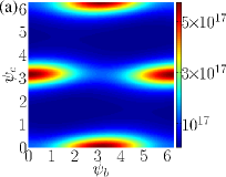
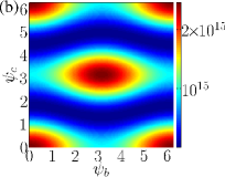
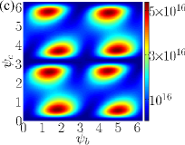
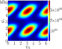
Figure 2: (color). Comparison of the perturbative and nonperturbative approach. Shown is the laboratory frame rate $d\dot{W}/d\omega_{b}d\Omega_{b}d\Omega_{c}$, in units of s^-1sr^-2MeV^-1, for the nonperturbative [(a), (c)] and perturbative [(b), (d)] case. The parameters employed are $E_{i}=10^{3}m$, $\omega=2.5$ eV, $\xi=1$, $\omega_{b}=1$ MeV, and $\theta_{b}=\theta_{c}=10^{-3}$. The photon polarizations are given by $\epsilon_{b,c}=\epsilon_{b,c}^{1}$ in (a) and (b), and $\epsilon_{b,c}=\epsilon_{b,c}^{2}$ in (c) and (d).

To answer the question whether the integrated nonperturbative rate differ significantly from the one predicted by the usual double Compton scattering formula, we show in Fig. 3 the differential rate $d\dot{W}/d\theta_{c}$, integrated over the azimuth angles $\psi_{b,c}$, the polar angle $\theta_{b}$ of one of the final photons and the energy $\omega_{b}$, and summed over the final photon polarizations. The energy integration was limited to the interval between 1 keV and 1 MeV to avoid the infrared divergence at $\omega_{b}\to 0$ BrFey1952 and cascade contributions for larger $\omega_{b}$, and for the same reason the integration over $\theta_{b}$ was performed over the interval $(0,1.5\times 10^{-3})$ radians. Restricting the final phase space in this way ensures that contributions from single Compton scattering are negligible; at polar angles smaller than $1.5\times 10^{-3}$ radians all harmonics occur at energies larger than 1 MeV. Integrating the nonperturbative curve in Fig. 3, we obtain a total rate in the laboratory frame of $\dot{W}=3.5\times 10^{7}$ s^-1. For the perturbative curve, we get $\dot{W}_{\textrm{pert}}=2.5\times 10^{7}$ s^-1, from which we gather that even for the integrated rate, the nonperturbative corrections are significant. The obtained two-photon rate should be compared to the total rate of nonlinear single Compton scattering NiRi1964 , which amounts to $3\times 10^{13}$ s^-1 for the same parameters as in Fig. 3. Employing an electron beam with $10^{9}$ electrons per bunch, a laser pulse of duration $100$ fs, photon energy $\omega=2.5$ eV, intensity $5.5\times 10^{18}$ W/cm² (corresponding to $\xi=1$) VULCAN , and assuming perfect transverse overlap of the two pulses, we estimate that about $2\times 10^{3}$ photon pairs per shot may be expected.

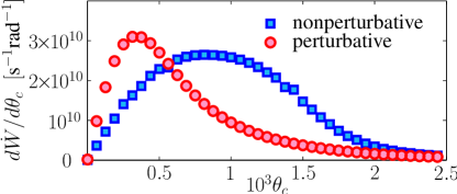
Figure 3: (color online). The integrated and polarization-summed lab-frame rate $d\dot{W}/d\theta_{c}=\sin\theta_{c}d\dot{W}/d\cos\theta_{c}$, differential only in the angle $\theta_{c}$. Shown are results for the perturbative and the nonperturbative calculations, for $E_{i}=10^{3}m$, $\omega=2.5$ eV, $\xi=1$.

Entanglement.—Having investigated the differential and total photon pair production rate, we now turn to the interesting question of the quantum mechanical correlation between the final state photons. To quantify the degree of polarization entanglement, we employ the well-established concurrence $C(\rho_{f})$ Wootters1998 as an entanglement measure. Assuming an unpolarized initial electron and unobserved final spin, we trace out the spin polarizations of the initial and final electron and calculate the $4\times 4$ final density matrix $\rho_{f}$ of the polarizations $\lambda_{b,c}\in\{1,2\}$ of the two emitted photons. Then, $C(\rho_{f})$ is given by

$$C(\rho_{f})=\textrm{max}(0,\sqrt{\zeta_{1}}-\sqrt{\zeta_{2}}-\sqrt{\zeta_{3}}-\sqrt{\zeta_{4}}),$$ (4)

where the $\zeta_{j}$’s are the eigenvalues, in descending order, of the matrix $Q=\rho_{f}(\sigma_{y}\otimes\sigma_{y})\rho_{f}^{\ast}(\sigma_{y}\otimes\sigma_{y})$, where $\sigma_{y}$ is the second Pauli matrix. For a maximally entangled state, $C(\rho_{f})=1$, and for a non-entangled state $C(\rho_{f})=0$. We note that the concurrence has recently been used to study correlation in the two-photon decay of a bound state radtke2008 . For the present case, the final density matrix $\rho_{f}$ can be computed from the normalized matrix element (Nonperturbative Treatment of Double Compton Backscattering in Intense Laser Fields). Writing $S=S_{r_{i},r_{f}}(\lambda_{b},\lambda_{c})$, where $r_{i}$ ($r_{f}$) denotes the spin polarization of the initial (final) electron, we have for the matrix elements of $\rho_{f}$,

$$\langle\lambda_{b},\lambda_{c}|\rho_{f}|\lambda^{\prime}_{b},\lambda^{\prime}_{c}\rangle=\frac{N}{2}\sum_{r_{i},r_{f}}S_{r_{i},r_{f}}(\lambda_{b},\lambda_{c})S^{\ast}_{r_{i},r_{f}}(\lambda^{\prime}_{b},\lambda^{\prime}_{c}).$$ (5)

Here $N$ is a normalization constant, which can be found by requiring $\mathrm{Tr}\,\rho_{f}=1$. The concurrence, as defined in Eq. (4), is a gauge invariant quantity, furthermore it does not depend on the basis used to describe the polarization of the photons $k_{b,c}$. $C(\rho_{f})$ depends sensitively on the energy and the directions of the emitted photons. One example of the fully differential concurrence is displayed in Fig. 4, which shows the necessity of the nonperturbative formalism to predict the degree of entanglement.

      

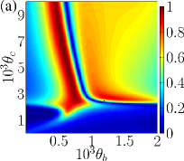
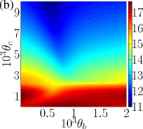
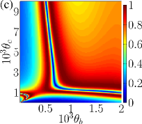
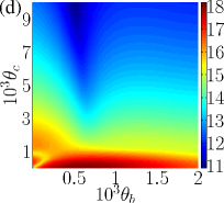
Figure 4: (color). In panel (a) we show the concurrence $C(\rho_{f})$ [see Eq. (4)], using the nonperturbative expression for the matrix element, which should be compared to panel (c), where the concurrence is shown for the perturbative case. The parameters employed are $E_{i}=10^{3}m$, $\omega=2.5$ eV, $\xi=1$, $\omega_{b}=1$ MeV, and $\psi_{b}=\psi_{c}=0$. As a reference, we also display in the right column the logarithm of the polarization-summed differential rate $\log_{10}(d\dot{W}/d\omega_{b}d\Omega_{b}d\Omega_{c})$, in units of s^-1sr^-2MeV^-1, for the nonperturbative [(b)] and perturbative [(d)] case.

Conclusions.—We have studied the process of nonperturbative two-photon decay of a laser-dressed electron. Our results significantly alter the theoretical predictions as compared to a perturbative treatment of the laser; they lead to novel features in the angular and integral characteristics, which could be resolved using presently available intense laser facilities.

- (1) O. Klein and T. Nishina, Z. Phys. A 52, 853 (1929).
- (2) N. B. Narozhnyĭ and M. S. Fofanov, JETP 83, 14 (1996).
- (3) L. S. Brown and T. W. B. Kibble, Phys. Rev. 133, A705 (1964).
- (4) M. Babzien et al., Phys. Rev. Lett. 96, 054802 (2006).
- (5) C. Bamber et al., Phys. Rev. D 60, 092004 (1999).
- (6) A. Zeilinger, Rev. Mod. Phys. 71, S288 (1999).
- (7) V. Yanovsky et al., Opt. Express 16, 2109 (2008).
- (8) C. Müller, Phys. Lett. B 672, 56 (2009).
- (9) D. L. Burke et al., Phys. Rev. Lett. 79, 1626 (1997).
- (10) H. R. Reiss, J. Math. Phys. 3, 59 (1962).
- (11) F. Mandl and T. H. R. Skyrme, Proc. Roy. Soc. London A 215, 497 (1952).
- (12) F. Bell, eprint arXiv:0809.1505v1 [quant-ph].
- (13) P. E. Cavanagh, Phys. Rev. 87, 1131 (1952).
- (14) M. B. Saddi et al., Nucl. Instrum. Meth. B 266, 3309 (2008).
- (15) R. Schützhold and C. Maia, Eur. Phys. J. D (2009), at press DOI: 10.1140/epjd/e2009-00038-4.
- (16) R. Schützhold et al., Phys. Rev. Lett. 97, 121302 (2006).
- (17) R. Schützhold et al., Phys. Rev. Lett. 100, 091301 (2008).
- (18) V. N. Baier et al., Phys. Rep. 78, 293 (1981).
- (19) D. L. Kahler et al., Phys. Rev. Lett. 68, 1690 (1992).
- (20) A. V. Korol and I. A. Solovjev, Rad. Phys. Chem. 75, 1346 (2006).
- (21) P. I. Fomin and R. I. Kholodov, JETP 96, 315 (2003).
- (22) A. A. Sokolov et al., Rus. Phys. J. 19, 1139 (1976).
- (23) D. A. Morozov and V. I. Ritus, Nucl. Phys. B 86, 309 (1975).
- (24) H. R. Reiss and J. H. Eberly, Phys. Rev. 151, 1058 (1966).
- (25) E. Lötstedt et al., New J. Phys. 11, 013054 (2009).
- (26) A. I. Nikishov and V. I. Ritus, Sov. Phys. JETP 19, 529 (1964).
- (27) H. J. Korsch et al., J. Phys. A 39, 14947 (2006).
- (28) W. Becker and H. Mitter, J. Phys. A 9, 2171 (1976).
- (29) U. D. Jentschura, Phys. Rev. A 79, 022510 (2009).
- (30) P. G. Thirolf et al., Eur. Phys. J. D (2009), at press DOI: 10.1140/epjd/e2009-00149-x.
- (31) G. Brodin et al., Class. Quantum Grav. 25, 145005 (2008).
- (32) L. M. Brown and R. P. Feynman, Phys. Rev. 85, 231 (1952).
- (33) http://www.clf.rl.ac.uk/Facilities/vulcan/laser.htm.
- (34) W. K. Wootters, Phys. Rev. Lett. 80, 2245 (1998).
- (35) T. Radtke et al., Phys. Rev. A 77, 022507 (2008).