Event-Driven Optimal Feedback Control for Multi-Antenna Beamforming

Abstract

Transmit beamforming is a simple multi-antenna technique for increasing throughput and the transmission range of a wireless communication system. The required feedback of channel state information (CSI) can potentially result in excessive overhead especially for high mobility or many antennas. This work concerns efficient feedback for transmit beamforming and establishes a new approach of controlling feedback for maximizing net throughput, defined as throughput minus average feedback cost. The feedback controller using a stationary policy turns CSI feedback on/off according to the system state that comprises the channel state and transmit beamformer. Assuming channel isotropy and Markovity, the controller’s state reduces to two scalars. This allows the optimal control policy to be efficiently computed using dynamic programming. Consider the perfect feedback channel free of error, where each feedback instant pays a fixed price. The corresponding optimal feedback control policy is proved to be of the threshold type. This result holds regardless of whether the controller’s state space is discretized or continuous. Under the threshold-type policy, feedback is performed whenever a state variable indicating the accuracy of transmit CSI is below a threshold, which varies with channel power. The practical finite-rate feedback channel is also considered. The optimal policy for quantized feedback is proved to be also of the threshold type. The effect of CSI quantization is shown to be equivalent to an increment on the feedback price. Moreover, the increment is upper bounded by the expected logarithm of one minus the quantization error. Finally, simulation shows that feedback control increases net throughput of the conventional periodic feedback by up to $0.5$ bit/s/Hz without requiring additional bandwidth or antennas.

I Introduction

Transmit beamforming is a popular multi-antenna technique for enhancing the reliability and throughput of a wireless communication link [1]. In many systems, transmit beamforming requires feedback of channel state information (CSI), incurring significant overhead especially for a large number of transmit antennas or fast fading [2, 3]. In this paper, we consider the transmit beamforming system and propose a new approach of maximizing net throughput, defined as throughput minus average feedback cost, via optimal feedback control. The controller under consideration turns CSI feedback on/off by observing the current system state that consists of the current channel state and transit beamformer. The optimal stationary control policy is shown to be of the threshold type. As a result, feedback is performed whenever transmit CSI is sufficiently outdated as measured by an optimal threshold function. Optimal feedback control is observed to substantially increase net throughput of the transmit beamforming system compared with the conventional periodic feedback [4, 2, 5].

I-A Prior Works

In multi-antenna systems, adaptive transmission techniques such as beamforming and precoding typically require periodic feedback of complex vectors or matrices derived from CSI. The potentially large feedback overhead has motivated active research on intelligent algorithms for quantizing feedback CSI, forming a research area called limited feedback [3]. Different approaches for quantizing CSI have been proposed, including line packing [4, 5], combined channel parameterization and scalar quantization [6], subspace interpolation [7], and Lloyd’s algorithm [8, 9]. Furthermore, various types of limited feedback systems have been designed, namely beamforming [4, 5], precoded orthogonal space-time block codes [10], precoded spatial multiplexing [11], and multiuser downlink [12]. The practicality of limited feedback has been recognized by the industry and related techniques have been integrated into latest wireless communication standards such as IEEE 802.16 [13] and 3GPP LTE [14].

Besides quantization, CSI feedback can be compressed by exploiting channel temporal correlation [6, 15, 16]. In [6], each CSI matrix for a multiple-input-multiple-output (MIMO) channel is parameterized and the parameters are sent back incrementally using the delta modulation. In [15], the feedback CSI matrix is compressed to be one bit indicating the channel variation with respect to a reference matrix sent by the transmitter. A lossy feedback compression algorithm is proposed in [16], which reduces feedback overhead by omitting in feedback the infrequent transitions between CSI states. In view of prior works, it remains unknown that how the average feedback cost can be minimized for given throughput.

The applications of opportunism [17, 18] to CSI feedback have resulted in opportunistic feedback algorithms for reducing sum feedback overhead in multi-user multi-antenna systems [19, 20, 21, 22, 23]. The common feature of these algorithms is that CSI feedback is performed only if a channel quality indicator exceeds a fixed threshold. Compared with periodic feedback over dedicated channels (see e.g. [4, 5]), opportunistic (aperiodic) feedback is much more efficient in terms of sum feedback overhead and thus is suitable for systems where users randomly access a common feedback channel. The thresholds for opportunistic feedback can be computed iteratively for maximizing throughput as in [19, 20] or derived in closed-form expressions for achieving optimal capacity scaling for asymptotically large numbers of users [24, 21, 22, 23]. For simplicity, the temporal correlation in practical channels is omitted in existing designs where independent block fading is assumed. Thus the existing opportunistic feedback algorithms are incapable of adapting feedback thresholds to channel dynamics for further feedback reduction.

The common objective of the works mentioned above is to maximize throughput. This performance metric fails to account for feedback cost though feedback competes with data transmission for resources including time, bandwidth and power. Thus net throughput defined earlier is a more practical metric. In [25, 26, 27], net throughput is maximized by optimizing the resource allocation to data transmission and feedback. In [25], a two-way beamforming system is considered, where data and CSI flow in both directions of the link between two multi-antenna transceivers. For this system, bounds on the feedback rate for maximizing net throughput are derived. For a similar system, net throughput is maximized in [26] by optimizing power allocation to training, feedback and data transmission. Net throughput optimization for the beamforming system is also investigated in [27] in terms of optimal bandwidth allocation to feedback and data transmission. Aligned with the direction of prior works, the current paper addresses net throughput maximization for transmit beamforming from the new perspective of feedback control, which adapts the mentioned resource allocation to channel dynamics.

I-B Contributions and Organization

In this paper, we consider a single-user transmit beamforming system with multiple transmit and a single receive antennas. Each feedback instant incurs fixed cost in bit/s/Hz, called feedback price. A feedback controller turns the feedback link either on or off such that net throughput is maximized. This work is based on the following assumptions. First, channel realizations form a stationary Markov chain. Second, the channel coefficients are i.i.d. complex Gaussian random variables. This assumption allows the state of the feedback controller to reduce to two scalars $g$ and $z$ without compromising the controller’s optimality. The parameter $g$ is the channel power and $z$ the squared cosine of the angle between the transmit beamformer and the channel vector. Large $z$ indicates accurate transmit CSI and vice versa [4, 5]. Finally, the distribution of $z$ in the next slot conditioned on a realization $a$ in the current slot is assumed to stochastically dominate the counterpart conditioned on $b\leq a$ [28]. Essentially, this assumption implies that $z$ being large in a slot likely remains large in the next slot.

The contributions of this paper are summarized as follows. In general, the paper establishes a new approach for controlling feedback for transmit beamforming to maximize net throughput. To efficiently compute the optimal control policy using dynamic programming (DP) [29], the state space of the controller, namely the product space of $(g,z)$, is quantized. Consider the perfect feedback channel free of feedback error. First, given the quantized state space, the feedback control policy for maximizing net throughput is proved to be of the threshold type. Specifically, feedback is performed only if $z$ is below the optimal threshold that depends on $g$. Second, the threshold type policy is proved to be optimal for feedback control with the continuous (unquantized) state space. Next, we consider the finite feedback channel that requires feedback CSI quantization. Fourth, the optimality of the threshold-type feedback control policy is proved for quantized feedback. Feedback CSI quantization reduces the receive SNR and also varies the dynamics of $z$. Fifth, to gain insight into these two effects, they are treated separately and each of them is shown to decrease net throughput. Finally, we show that the effect of CSI quantization on net throughput can be interpreted as an increment on the feedback price. This increment is upper bounded by the expected logarithm of one minus the quantization error.

Simulation results are also presented for the channel model specified by i.i.d. Rayleigh fading and Clarke’s temporal correlation. Define the feedback gain as throughput for free feedback minus that for no feedback. With respect to periodic feedback, optimal controlled feedback is observed to increase the feedback gain by up to $0.5$ bit/s/Hz, equal to $24\%$ of the feedback gain. The increase in net throughput is insensitive to the variation on Doppler frequency and the number of transmit antennas. For both perfect and imperfect feedback channels, the optimal feedback control policies computed numerically are observed to exhibit the threshold structure as predicted analytically. Moreover, the feedback threshold decreases with the increasing feedback price, corresponding to less frequent feedback. Last, feedback quantization is observed to reduce ergodic throughput as well as the feedback threshold, decreasing the feedback frequency.

The remainder of this paper is organized as follows. The system model is described in Section II. The optimal feedback control policies for the perfect and finite-rate feedback channels are analyzed in Section IV and V, respectively. Simulation results are presented in Section VI followed by concluding remarks in Section VII.

Notation: A matrix is represented by a boldface capitalized letter and a vector by a boldface small letter. The $(m,n)$th element of a matrix ${\mathbf{X}}$ is represented by $[{\mathbf{X}}]_{m,n}$. For a vector ${\mathbf{x}}$, $[{\mathbf{x}}]_{m}$ gives the $m$th element. The superscript $\dagger$ denotes the complex conjugate transpose operation on a matrix or a vector. Define the operator $(a)^{+}$ on a scalar $a$ as $(a)^{+}:=\max(0,a)$. The realization of a stochastic process in the $t$th time slot is specified by the subscript $t$.

II System Model

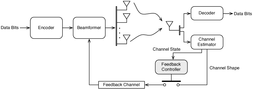
Figure 1: Transmit beamforming system with controlled CSI (channel shape) feedback

We consider the transmit beamforming system illustrated in Fig. 1, where a transmitter with $L$ antennas transmits to a receiver with a single antenna. The frequency-flat channel is a $L\times 1$ complex vector denoted as ${\mathbf{h}}$. To facilitate our designs, ${\mathbf{h}}$ is decomposed into the channel power $g:=\|{\mathbf{h}}\|^{2}$ and the channel shape ${\mathbf{s}}:={\mathbf{h}}/\|{\mathbf{h}}\|$, which are the indicators of the channel quality and direction, respectively. It follows that ${\mathbf{h}}=\sqrt{g}{\mathbf{s}}$. It is well-known that applying ${\mathbf{s}}$ as the beamforming vector, denoted as ${\mathbf{f}}$, maximizes the receive signal-to-noise ratio (SNR) [1]. To this end, ${\mathbf{s}}$ is estimated by the receiver at the beginning of each time slot of $T_{c}$ seconds and communicated to the transmitter via the feedback channel. The channel is assumed constant within each slot and thus feedback is performed at most once per slot. Depending on the channel state ${\mathbf{h}}$ (or $g$ and ${\mathbf{s}}$), the feedback controller turns CSI feedback on/off at the beginning of each time slot. Let $\mathcal{U}:=\{0,1\}$ denote the control state space and $\mu\in\mathcal{U}$ the feedback decision, where $1$ and $0$ correspond to the on and off states of the feedback link. Define the controller’s state $x:=(g,{\mathbf{s}},{\mathbf{f}})$ that contains all system variables affecting net throughput obtained in the sequel. Thus the state space is $\mathcal{X}:=\mathds{R}^{+}\times\mathds{O}^{L}\times\mathds{O}^{L}$ where $\mathds{O}^{L}$ represents the unit hypersphere embedded in $\mathds{C}^{L}$ [5]. We consider a stationary feedback control policy $\mathcal{P}:\mathcal{X}\rightarrow\mathcal{U}$ independent of the slot index $t$ [29]. It is assumed that per usage of the feedback channel incurs the feedback cost of $B$ bit. Moreover, the transmission time of feedback CSI is assumed negligible. We consider long data codewords covering many channel realizations. Given channel ergodicity and stationary feedback control, the net throughput in bit/s can be written as [25]

$$R=\frac{1}{T_{s}}\mathbb{E}\left[\log_{2}(1+Pg|{\mathbf{s}}^{\dagger}{\mathbf{f}}|^{2})\right]-\frac{B}{T_{c}}\Pr(\mu=1)$$ (1)

where $P$ is the transmit SNR and $T_{s}$ the symbol duration. For simplicity, net throughput can be written in bit/s/Hz as

$$J=\mathbb{E}\left[\log_{2}(1+Pg|{\mathbf{s}}^{\dagger}{\mathbf{f}}|^{2})\right]-\alpha\Pr(\mu=1)$$ (2)

where $\alpha:=\frac{BT_{s}}{T_{c}}$ is called the feedback price.

The feedback controller controls the transmit beamformer via feedback and thereby influences the receive SNR. Define $z:=|{\mathbf{s}}^{\dagger}{\mathbf{f}}|^{2}$ that represents the controllable component of the receive SNR $\mathsf{SNR}_{r}=Pgz$ [4, 5]. Consider the perfect feedback channel. The temporal variation of $z$ under feedback control is illustrated in Fig. 2. Upon CSI feedback, ${\mathbf{f}}$ is updated with ${\mathbf{s}}$ and the value of $z$ is reset to the maximum of one; if feedback is turned off, $z$ is smaller than one due to that ${\mathbf{f}}$ fails to adapt instantaneously to the time varying ${\mathbf{s}}$. With ${\mathbf{f}}$ fixed, the probability density function (PDF) of $z$ is referred to as the uncontrolled PDF and denoted as $\check{f}(z\mid{\mathbf{f}})$. The uncontrolled PDF governs the dynamics of $z$ between two consecutive feedback instants (cf. Fig. 2). The random variable $z$ is used later as a controller state variable. In addition, besides the mentioned perfect feedback channel, the one with a finite-rate constraint is also considered in the sequel.

Figure 2: Temporal variation of $z$ under feedback control

We make several assumptions on the channel distribution as described shortly. These assumptions facilitate computing the optimal feedback control policy $\mathcal{P}^{\star}$ using DP [29] and analyzing the policy structure. Model the channel as a stochastic sequence denoted as ${\mathbf{h}}_{0},{\mathbf{h}}_{1},{\mathbf{h}}_{2},\dots$, where ${\mathbf{h}}_{t}$ is the channel state in the $t$th slot.

Assumption 1

The sequence ${\mathbf{h}}_{0},{\mathbf{h}}_{1},{\mathbf{h}}_{2},\dots$ is a stationary Markov chain.

In other words, given ${\mathbf{h}}_{n}$, ${\mathbf{h}}_{n+1}$ is independent of the past realizations ${\mathbf{h}}_{n-1},{\mathbf{h}}_{n-2},\cdots$. Markov chains are commonly used for modeling temporally-correlated wireless channels (see e.g., [30, 31, 32, 33, 34]). Markov channel models have been validated both analytically (see e.g., [30, 35]) and by measurement [36]. Next, the controller’s state space $\mathcal{X}$ have $(2L+1)$ dimensions. Due to the curse of dimensionality, computing $\mathcal{P}^{\star}$ is impractical if $L$ is large [29]. The following assumption overcomes this difficulty, which is commonly made in the literature (see e.g. [37, 38]).

Assumption 2

The channel ${\mathbf{h}}$ comprises i.i.d. $\mathcal{CN}(0,1)$ random variables.

Given this assumption, $g$ follows chi-square distribution with $L$ complex degrees of freedom [39]; ${\mathbf{s}}$ is isotropic. As a result, the uncontrolled distribution of $z$ is independent of ${\mathbf{f}}$ and hence we can write $\check{f}(z\mid{\mathbf{f}})$ as $\check{f}(z)$. It follows that the state variables ${\mathbf{s}}$ and ${\mathbf{f}}$ can be combined into $z$. Thus the controller’s state and state space reduce to $x=(g,z)$ and $\mathcal{X}=\mathds{R}^{+}\times\mathcal{Z}$ with $\mathcal{Z}:=[0,1]$, respectively, thereby overcoming the mentioned curse of dimensionality. We make the following assumption on the temporal correlation of $z$ that affects the structure of $\mathcal{P}^{\star}$ (cf. Section IV).

Assumption 3

For $1\geq a\geq b\geq 0$, the uncontrolled distribution of $z_{t+1}$ conditioned on $z_{t}=a$ is stochastically dominant [28] over that conditioned on $z_{t}=b$. Mathematically,

$$\int_{c}^{\infty}\check{f}(z_{t+1}\mid z_{t}=a)dz_{t+1}\geq\int_{c}^{\infty}\check{f}(z_{t+1}\mid z_{t}=b)dz_{t+1}$$

where $0\leq c\leq 1$.

This assumption essentially states that large $z_{t}$ likely leads to large $z_{t+1}$ and vice versa, which is reasonable given channel temporal correlation. This work requires no assumption on the temporal correlation of $g$.

Finally, let $f(z_{t+1}\mid z_{t},\mu_{t})$ and $\tilde{f}(g_{t+1}\mid g_{t})$ denote the transition PDF’s of $z$ and $g$ respectively. For convenience, the state transition PDF is written as $f_{x}:=\tilde{f}\times f$.

III Problem Formulation

In this section, the problems of optimal feedback control are formulated and solved in the subsequent sections. Both perfect and finite-rate feedback channels are considered in the problem formulation.

The generic average and discounted reward problems are defined as follows [29]. By abuse of notation, the symbols in the preceding section are reused here. Consider a dynamic system with an infinite number of stages (infinite horizon), a state space $\mathcal{X}$ and a control space $\mathcal{U}$. The system dynamics are specified by the state transition kernel $f_{x}(x_{t}\mid x_{t},\mu_{t})$ with $x\in\mathcal{X}$ and $\mu\in\mathcal{U}$. The reward-per-stage is represented by the function $G:\mathcal{X}\times\mathcal{U}\rightarrow\mathds{R}^{+}$. The control policy $\mathcal{P}:\mathcal{X}\rightarrow\mathcal{U}$ is optimized for maximizing either the average reward

$$J:=\lim_{T\rightarrow\infty}\frac{1}{T}\sum_{t=0}^{T-1}G(x_{t},\mu_{t})$$ (3)

or the discounted reward

$$J_{\beta}(x_{0}):=\sum_{t=0}^{\infty}\beta^{t}\mathbb{E}[G(x_{t},\mu_{t})\mid x_{0}]$$ (4)

where $0<\beta<1$ is the discount factor. This corresponding optimization problems are called the infinite-horizon average and discounted reward problems represented by $\mathcal{A}(\mathcal{X},\mathcal{U},f_{x},G)$ and $\mathcal{D}(\mathcal{X},\mathcal{U},f_{x},G)$, respectively. These problems can be solved iteratively using DP [29].

Consider the perfect feedback channel. Net throughput in (2) can be written as the average reward in (3) with $G$ given by

$$G(g,z,\mu):=\left\{\begin{aligned} &\log_{2}(1+Pg)-\alpha,&&\mu=1\\ &\log_{2}(1+Pgz),&&\textrm{otherwise}.\end{aligned}\right.$$ (5)

Hereafter the terms, average reward and net throughput, are used interchangeably. Thus the feedback controller can be designed by solving $\mathcal{A}(\mathcal{X},\mathcal{U},f_{x},G)$ with $f_{x}$ obtained as follows

$$f_{x}(x_{t+1}\mid x_{t},\mu_{t}) = f_{x}((g_{t+1},z_{t+1})\mid(g_{t},z_{t}))$$ (6)

$$= \tilde{f}(g_{t+1}\mid z_{t+1},g_{t},z_{t},\mu_{t})f(z_{t+1}\mid g_{t},z_{t},\mu_{t})$$

$$\overset{(a)}{=} \tilde{f}(g_{t+1}\mid g_{t})f(z_{t+1}\mid z_{t},\mu_{t})$$

where $(a)$ follows from the channel isotropy. From the discussion in Section II

$$f(z_{t+1}\mid z_{t}=c,\mu_{t})=\left\{\begin{aligned} &\check{f}(z_{t+1}\mid z_{t}=1),&&\mu_{t}=1,\\ &\check{f}(z_{t+1}\mid z_{t}=c),&&\textrm{otherwise}\end{aligned}\right.$$ (7)

with $c\in\mathcal{Z}$. The optimal policy $\mathcal{P}^{\star}$ for solving $\mathcal{A}(\mathcal{X},\mathcal{U},f_{x},G)$ is analyzed in Section IV.

In practice, CSI feedback is mplemented using a narrow-band (finite-rate) control channel [14, 13, 2]. The finite-rate feedback constraint requires quantizing feedback CSI as described shortly. Let $\hat{{\mathbf{s}}}$ denote the $L\times 1$ complex unitary vector resulting from quantizing ${\mathbf{s}}$ [4, 5]. We consider a codebook based quantizer where the codebook $\mathcal{F}$ is a set of complex unitary vectors [4, 5]. Using $\mathcal{F}$, $\hat{{\mathbf{s}}}$ is obtained by quantizing ${\mathbf{s}}$ using the maximum SNR criterion, namely that $\hat{{\mathbf{s}}}=\max_{{\mathbf{x}}\in\mathcal{F}}|{\mathbf{s}}^{\dagger}{\mathbf{x}}|^{2}$. Define $\epsilon:=|\hat{{\mathbf{s}}}^{\dagger}{\mathbf{s}}|^{2}$ where $0\leq\epsilon\leq 1$. This scalar quantifies the loss on the receive SNR $(\mathsf{SNR}_{\epsilon}=Pg\epsilon)$ upon CSI feedback compared with that $(\mathsf{SNR}=Pg)$ for the perfect feedback channel [5, 4, 40]. Note that $\epsilon$ is equal to one minus the quantization error defined in [42, 40]. The distribution of $\epsilon$ depends on the channel distribution and design of the quantizer codebook [4, 5, 40]. Again, net throughput maximization is formulated as an average reward problem. This problem differs from $\mathcal{A}(\mathcal{X},\mathcal{U},f_{x},G)$ for perfect feedback only in the state transition kernel and award-per-stage. The transition PDF of $z$ is obtained as

$$f_{\epsilon}(z_{t+1}\mid z_{t}=c,\mu_{t})=\left\{\begin{aligned} &\underset{\epsilon}{\mathbb{E}}[\check{f}(z_{t+1}\mid z_{t}=\epsilon)],&&\mu_{t}=1,\\ &\check{f}(z_{t+1}=a\mid z_{t}=c),&&\textrm{otherwise}\end{aligned}\right.$$ (8)

where $\underset{\epsilon}{\mathbb{E}}$ denotes the expectation over the distribution of $\epsilon$. Thus for the corresponding average reward problem, the state transition kernel is $f_{x}^{\epsilon}=\tilde{f}\times f_{\epsilon}$. Given the receive SNR $\mathsf{SNR}_{\epsilon}=Pg\epsilon$ upon CSI feedback, the reward-per-stage function $G_{\epsilon}$ is modified from (5) as

$$G_{\epsilon}(x,\mu):=\left\{\begin{aligned} &\underset{\epsilon}{\mathbb{E}}[\log_{2}(1+Pg\epsilon)]-\alpha,&&\mu=1,\\ &\log_{2}(1+Pgz),&&\textrm{otherwise}.\end{aligned}\right.$$ (9)

In Section V, we consider $\mathcal{A}(\mathcal{X},\mathcal{U},f_{x}^{\epsilon},G_{\epsilon})$ and analyze the resultant optimal policy.

IV Feedback Control Policy: Perfect Feedback Channel

In this section, the optimal feedback control policy is analyzed for the perfect feedback channel. To compute the policy using DP, the state space of the feedback controller is quantized. Given the discrete state space, the optimal control policy is proved to be of the threshold type. This policy structure is shown to also hold for the optimal feedback control with the continuous state space.

IV-A State-Space Quantization

The channel state $(g,z)\in\mathcal{X}$ is quantized as $(\hat{g},\hat{z})\in\hat{\mathcal{X}}$ that is used as the input of the feedback controller, where $\hat{\mathcal{X}}$ denote the discrete state space defined in the sequel. Feedback control with $\hat{\mathcal{X}}$ allows applying stochastic optimization theory to analyzing the optimal control policy in the sequel. The algorithms for quantizing $(g,z)$ are described as follows.

The space of $g$, namely the nonnegative real line $\mathds{R}^{+}$, is partitioned into $M$ line segments $[\tilde{g}_{0},\tilde{g}_{1})$, $[\tilde{g}_{1},\tilde{g}_{2})$, $\cdots$, $[\tilde{g}_{M-1},\infty)$, where $\tilde{g}_{0}=0$ and $0<\tilde{g}_{1}<\tilde{g}_{2}<\cdots<\tilde{g}_{M-1}<\infty$. The values of $\{\tilde{g}_{m}\}$ are chosen such that $g$ lies in different line segments with equal probabilities. In other words, $\Pr(G\in[\tilde{g}_{m},\tilde{g}_{m+1}))=\frac{1}{M}\ \forall\ 0\leq m\leq M-1$ with $\tilde{g}_{M}=\infty$. The above $M$ line segments are represented by a set of $M$ finite values $\hat{\mathcal{G}}=\{\bar{g}_{0},\bar{g}_{1},\cdots,\bar{g}_{M-1}\}$ called grid points [43], which are arbitrarily selected from corresponding segments and hence satisfy the constraints $\bar{g}_{m}\in[\tilde{g}_{m},\tilde{g}_{m+1}]\ \forall\ m$.  Similarly, the space of $z$, namely the line segment $\mathcal{Z}=[0,1]$, is divided into $N$ sub-segments of equal length $[\tilde{z}_{0},\tilde{z}_{1}),[\tilde{z}_{1},\tilde{z}_{2}),\cdots,[\tilde{z}_{N-1},\tilde{z}_{N}]$ where $\tilde{z}_{0}=0$ and $\tilde{z}_{N}=1$. Define the set $\tilde{\mathcal{Z}}:=\{\tilde{z}_{n}\}_{n=0}^{N}$. Again, $N$ grid points $\hat{\mathcal{Z}}=\{\bar{z}_{0},\bar{z}_{1},\cdots,\bar{z}_{N-1}\}$ are arbitrarily chosen from the $N$ sub-segments mentioned earlier. The discrete state space can be readily written as $\hat{\mathcal{X}}:=\hat{\mathcal{G}}\times\hat{\mathcal{Z}}$. The space $\mathcal{X}$ can be mapped to $\hat{\mathcal{X}}$ using the following quantization functions $\mathcal{Q}_{g}$ and $\mathcal{Q}_{z}$

$$\hat{g}=\mathcal{Q}_{g}(g) = \bar{g}_{m},\quad g\in[\tilde{g}_{m},\tilde{g}_{m+1})$$ (10)

$$\hat{z}=\mathcal{Q}_{z}(z) = \bar{z}_{n},\quad z\in[\tilde{z}_{n},\tilde{z}_{n+1}).$$ (11)

Note that the above quantization algorithms are used for simplicity and only one of many designs that lead to the same results as obtained in the following sections.

Given Assumption 1, the sequences $\{\hat{g}_{t}\}$ and $\{\hat{z}_{t}\}$ are two Markov chains with the discrete state spaces $\hat{\mathcal{G}}$ and $\hat{\mathcal{Z}}$, respectively. The transition probabilities of the two Markov chains are decoupled as a result of (6). For $\{\hat{z}_{t}\}$, let $P_{m,n}$ denote the probability for transition from the state $m$ to $n$ and $\mu$ the feedback decision corresponding to quantized controller input. Then $P_{m,n}$ can be written as a function of $\mu$

$$P_{m,n}(\mu):=\left\{\begin{aligned} &\int_{\tilde{z}_{n}}^{\tilde{z}_{n+1}}\check{f}(z_{t+1}=\tau\mid z_{t}=1)d\tau,&&\mu=1\\ &\int_{\tilde{z}_{n}}^{\tilde{z}_{n+1}}\check{f}(z_{t+1}=\tau\mid z_{t}=\bar{z}_{m})d\tau,&&\textrm{otherwise}\end{aligned}\right.$$ (12)

where $0\leq m,n\leq N-1$. Note that $P_{m,n}(1)$ is independent of $n$. Similarly, define the counterpart of $P_{m,n}$ for $\{\hat{g}_{t}\}$ as

$$\tilde{P}_{m,n}:=\int_{\tilde{g}_{n}}^{\tilde{g}_{n+1}}\tilde{f}(g_{t+1}=\tau\mid g_{t}=\bar{g}_{m})d\tau$$ (13)

where $0\leq m,n\leq M-1$. Note that $\tilde{P}_{m,n}$ are unaffected by feedback control. For convenience, define the transition probability matrix ${\mathbf{P}}$ with $[{\mathbf{P}}]_{m,n}:=P_{m,n}$ and similarly $\tilde{{\mathbf{P}}}$ with $[\tilde{{\mathbf{P}}}]_{m,n}:=\tilde{P}_{m,n}$. Due to feedback control, the stationary probabilities of $\hat{z}$ depend on those of $\hat{g}$. Thus we define the joint stationary probability $\pi_{m,n}:=\Pr(\hat{g}=\bar{g}_{m},\hat{z}=\bar{z}_{n})$ where $0\leq m\leq M-1,0\leq n\leq N-1$. With the discrete state space, the state transition kernel is denoted as ${\mathbf{P}}_{x}:=\tilde{{\mathbf{P}}}\times{\mathbf{P}}$.

The average reward problems $\mathcal{A}(\hat{\mathcal{X}},\mathcal{U},{\mathbf{P}}_{x},G)$ and $\mathcal{A}(\mathcal{X},\mathcal{U},f_{x},G)$ are considered in Section IV-B and IV-C, respectively. Let $\hat{J}^{\star}$ denote the maximum average reward for the discrete state space. Then $\hat{J}^{\star}$ is an approximation of $J^{\star}$ for the continuous state space. They converge as the quantization resolution increases: $M\rightarrow\infty,N\rightarrow\infty$ (cf. Section IV-C).

IV-B Policy for Discrete State Space

This section focuses on $\mathcal{A}(\hat{\mathcal{X}},\mathcal{U},{\mathbf{P}}_{x},G)$. The resultant optimal policy $\hat{\mathcal{P}}^{\star}$ is shown to be of the threshold type. In addition, the computation of $\hat{\mathcal{P}}^{\star}$ is discussed.

Rather than obtaining $\hat{\mathcal{P}}^{\star}$ directly, the policy $\hat{\mathcal{P}}^{\star}_{\beta}$ is derived by solving $\mathcal{D}(\hat{\mathcal{X}},\mathcal{U},{\mathbf{P}}_{x},G)$. Then the desired $\hat{\mathcal{P}}^{\star}$ follows from $\hat{\mathcal{P}}^{\star}_{\beta}$ by allowing $\beta\rightarrow 1$. The policy $\hat{\mathcal{P}}^{\star}_{\beta}$ can be found using DP [29]. To this end, define the DP operator $\mathsf{F}$ on a given function $q:\hat{\mathcal{X}}\rightarrow\mathds{R}^{+}$ as

$$(\mathsf{F}q)(\bar{g}_{m},\bar{z}_{n})=\max_{\mu\in\{0,1\}}\left[G(\bar{g}_{m},\bar{z}_{n},\mu)+\beta\sum\nolimits_{k,\ell}q(k,\ell)\tilde{P}_{k,m}P_{\ell,n}(\mu)\right]$$ (14)

where $0\leq m\leq M-1$ and $0\leq n\leq N-1$. The maximum discounted reward $\hat{J}_{\beta}^{\star}$ satisfies Bellman’s equation $\hat{J}_{\beta}^{\star}=\mathsf{F}\hat{J}_{\beta}^{\star}$ [29]. For convenience, represent $\hat{J}_{\beta}((\bar{g}_{m},\bar{z}_{n}))$ by $\hat{J}_{\beta}(m,n)$.

We refer to a $N\times N$ stochastic matrix ${\mathbf{A}}$ as being montone if ${\mathbf{A}}$ satisfies 

$$\sum_{m=m_{0}}^{N-1}[{\mathbf{A}}]_{m,n_{1}}\geq\sum_{m=m_{0}}^{N-1}[{\mathbf{A}}]_{m,n_{2}}\quad\textrm{if}\ 0\leq n_{2}\leq n_{2}\leq N-1$$ (15)

where $0\leq m_{0}\leq N-1$. Thus ${\mathbf{P}}$ is monotone following Assumption 3 and (12). Moreover, define a monotone vector of real numbers as one whose elements are in the ascending order. The following lemma is useful for the analysis in this paper.

Lemma 1

1. Consider a real vector ${\mathbf{v}}$ and a stochastic matrix ${\mathbf{A}}$ that are both monotone and have the same height. Then ${\mathbf{A}}^{\dagger}{\mathbf{v}}$ is a monotone vector;

2. Consider a matrix ${\mathbf{B}}$ of nonnegative elements and a matrix ${\mathbf{C}}$ with monotone rows. Then the rows of ${\mathbf{B}}{\mathbf{C}}$ are also monotone.

Proof: See Appendix -A.  $\Box$

The following lemma is essential for obtaining the main result of this section. The proof of Lemma 2 is based on value iteration [29]. Using this method, for an arbitrary function $q:\hat{\mathcal{X}}\rightarrow\mathds{R}^{+}$, the maximum discounted reward $\hat{J}_{\beta}^{\star}$ can be computed iteratively as

$$\hat{J}_{\beta}^{\star}(m,n)=\lim_{k\rightarrow\infty}(\mathsf{F}^{k}q)(m,n).$$ (16)

Lemma 2

$\hat{J}_{\beta}^{\star}$ has the following properties:

1. Given $\hat{g}$, $\hat{J}^{\star}_{\beta}(\hat{g},\hat{z})$ monotonically increases with $\hat{z}$;

2. Define $w(m,n,\mu):=\sum_{k,\ell}\hat{J}^{\star}_{\beta}(k,\ell)\tilde{P}_{m,k}P_{n,\ell}(\mu)$. Given $m$ and $\mu$, $w(m,n,\mu)$ monotonically increases with $n$;

3. Given $m$, $w(m,n,1)\geq w(m,n,0)\ \forall\ n$.

Proof: See Appendix -B.  $\Box$

Using the above lemma, the main result of this section is obtained as shown in the following theorem.

Theorem 1

The optimal policy $\hat{\mathcal{P}}^{\star}$ is of the threshold type. Specifically, there exists a function $\hat{y}:\hat{\mathcal{G}}\rightarrow\mathcal{Z}$ such that

$$\hat{\mathcal{P}}^{\star}:\mu=\left\{\begin{aligned} &0,&&\hat{z}\geq\hat{y}(\hat{g})\\ &1,&&\textrm{otherwise.}\end{aligned}\right.$$ (17)

The function $\hat{y}(\cdot)$ is bounded as

$$\left(\frac{2^{-\alpha}(1+P\hat{g})-1}{P\hat{g}}\right)^{+}\leq\hat{y}(\hat{g})\leq 1.$$ (18)

Proof: See Appendix -C.  $\Box$

Several remarks are in order.

1. Why the optimal policy has the threshold structure is explained as follows. Small $\hat{z}$ corresponds to outdated transmit CSI and vice versa. As a result, CSI feedback for small $\hat{z}$ yields significant reward-per-stage but that for large $\hat{z}$ may result in negative reward-per-stage due to the feedback cost. Therefore the optimal feedback policy should enable feedback only in the regime of small $\hat{z}$, resulting in the threshold-type policy. In addition, the feedback threshold on $\hat{z}$ depends on $\hat{g}$ since the reward-per-stage is a function of $\hat{g}$.

2. One would expect that larger $\hat{g}$ makes feedback more desirable because the resultant reward is also larger (cf. (5)). In other words, the threshold function $\hat{y}$ should monotonically increase with $\hat{g}$. This is observed in simulation. However, proving this property requires making an assumption on the temporal correlation of $g$, which, however, is unnecessary for this work.

3. The threshold lower bound in (18) corresponds to the feedback control policy that enables feedback whenever it gives larger reward-per-stage than no feedback. However, this policy is suboptimal because feedback may lead to extra reward in subsequent slots despite providing a smaller reward-per-stage in the current slot than no feedback. Therefore the optimal policy should support more frequent feedback than the above suboptimal one. This is the reason that the optimal threshold function is lower bounded as shown in (18).

4. For a high transmit SNR ($P\rightarrow\infty$), the award-per-stage in (5) can be approximated as

   $$G(\hat{g},\hat{z},\mu) = \left\{\begin{aligned} &\log_{2}(1+P\hat{g})-\alpha,&&\mu=1,\\ &\log_{2}(1/\hat{z}+P\hat{g})+\log_{2}\hat{z},&&\textrm{otherwise}\end{aligned}\right.$$ (19)

   $$\approx \left\{\begin{aligned} &\log_{2}(P\hat{g})-\alpha,&&\mu=1,\\ &\log_{2}(P\hat{g})+\log_{2}\hat{z},&&\textrm{otherwise}.\end{aligned}\right.$$ (20)

   Define $\Delta G(\hat{g},\hat{z}):=G(\hat{g},\hat{z},0)-G(\hat{g},\hat{z},1)$. From (20), $\Delta G(\hat{g},\hat{z})\approx\log_{2}\hat{z}+\alpha$ for $P\rightarrow\infty$. The optimal policy $\hat{\mathcal{P}}^{\star}$ essentially depends only on $\Delta G(\hat{g},\hat{z})$ and the dynamics of $\hat{z}$. Both factors are independent of $\hat{g}$ for $P\rightarrow\infty$. Consequently, the optimal threshold on $\hat{z}$ is insensitive to the variation on $\hat{g}$ for high SNR’s. This is confirmed by simulation as discussed in Section VI.

For the extreme cases of zero and infinite feedback prices, the feedback threshold is specified in the following corollary.

Corollary 1

The feedback threshold $\hat{y}$ is fixed at $\hat{y}=0$ for $\alpha=\infty$ and $\hat{y}=1$ for $\alpha=0$.

Proof: See Appendix -D  $\Box$

Note that $\hat{y}=0$ and $\hat{y}=1$ correspond to no feedback and feedback in every time slot, respectively. The above results agree with the intuition that feedback is undesirable when the feedback price is too high but feedback should be performed persistently if it is free.

Given the threshold function $\hat{y}$ defining $\hat{\mathcal{P}}^{\star}$ (cf. Theorem 1), the maximum award can be obtained as

$$\hat{J}^{\star}(\hat{y})=\sum_{m=0}^{M-1}\sum_{n=0}^{N-1}G(\bar{g}_{m},\bar{z}_{n},\check{\mu}_{m,n})\pi_{m,n}$$ (21)

where

$$\check{\mu}_{m,n}=\left\{\begin{aligned} &0,&&\bar{z}_{n}\geq\hat{y}(\bar{g}_{m}),\\ &1,&&\textrm{otherwise}\end{aligned}\right.$$ (22)

and the stationary probabilities $\{\pi_{m,n}\}$ are obtained by solving the following linear equations [44]

$$\pi_{m,n}=\sum_{k,\ell}\tilde{P}_{m,k}P_{n,\ell}(\check{\mu}_{m,n})\pi_{k,\ell}\quad\textrm{and}\quad\sum_{m,n}\pi_{m,n}=1.$$ (23)

Finally, we discuss the computation of $\hat{\mathcal{P}}^{\star}$. Let $\hat{{\mathbf{y}}}$ denote the $N\times 1$ threshold vector with $[\hat{{\mathbf{y}}}]_{n}=\hat{y}(\bar{g}_{n})$. Then ${\mathbf{y}}$ determining $\hat{\mathcal{P}}^{\star}$ can be computed either by an exhaustive search or policy iteration [29]. Using Theorem1 and (21), the brute force approach is specified by $\hat{{\mathbf{y}}}=\max_{{\mathbf{x}}\in\mathcal{V}}J^{\star}({\mathbf{x}})$ where $\mathcal{V}=\left\{{\mathbf{x}}\in\tilde{\mathcal{Z}}^{M}\mid[{\mathbf{x}}]_{m}\geq\left(\frac{2^{-\alpha}(1+P\bar{g}_{m})-1}{P\bar{g}_{m}}\right)^{+}\right\}$. For this approach, the threshold structure of $\hat{\mathcal{P}}^{\star}$ is exploited to reduce the complexity of the exhaustive search from $O(2^{MN})$ to $O(|\mathcal{V}|)=O(N^{M})$. However, this complexity is still too high if $M$ and $N$ are large. For this case, a more practical approach for computing ${\mathbf{y}}$ is policy iteration [29]. Each iteration comprises two steps, namely policy evaluation and policy improvement. The policy evaluation in the $i$th iteration is to evaluate a given policy $\hat{\mathcal{P}}^{(i)}$ by computing the average reward and a set of parameters $\{A_{m,n}\}$ called differential rewards as follows [29]

$$J^{(i+1)}+A^{(i+1)}_{m,n} = G(\bar{g}_{m},\bar{z}_{n},\mu_{m,n})+\sum_{k,\ell}A^{(i)}_{k,\ell}\tilde{P}_{k,m}P_{\ell,n}(\mu_{m,n}),\quad\forall\ m,n$$ (24)

$$A^{(k)}_{M-1,N-1} = 0$$ (25)

where $\mu_{m,n}$ denotes the decision for the state $(\hat{g},\hat{z})=(\bar{g}_{m},\bar{z}_{n})$. The subsequent policy improvement is specified by

$$\mu^{(i+1)}_{m,n}=\arg\max_{x\in\{0,1\}}\left[G(\bar{g}_{m},\bar{z}_{n},x)+\sum_{k,\ell}A^{(i)}_{k,\ell}\tilde{P}_{k,m}P_{\ell,n}(x)\right],\quad\forall\ m,n.$$ (26)

The policy iteration terminates if $\mu^{(i+1)}_{m,n}=\mu^{(i)}_{m,n}\ \forall\ m,n$. For the simulation in Section VI, the policy iteration converges typically within several iterations.

IV-C Policy for Continuous State Space

In this section, we consider the case where $(g,z)$ is directly used as the controller input and design the controller by solving $\mathcal{A}(\mathcal{X},\mathcal{U},f_{x},G)$. The resultant optimal feedback control policy $\mathcal{P}^{\star}$ is proved to be of the threshold type. Specifically, we show that the threshold structure of $\hat{\mathcal{P}}^{\star}$ as given in Theorem 1 holds in the limit of high quantization resolution ($M\rightarrow\infty$ and $N\rightarrow\infty$).

The proof of this result uses those in [43], which addresses the validity of approximately solving a discounted-reward (or discounted-cost) problem with a continuous state space by quantizing the space and using DP. A key result in [43] states that the approximate solution converges to the continuous-space counterpart as the space-quantization error reduces to zero. This requires that the reward-per-stage and the state transition kernel are Lipschitz continuous. To state this result mathematically, some notation is introduced. Consider an infinite-horizon discounted reward problem with a compact state space $\mathcal{X}^{\prime}$ and a finite control space $\mathcal{U}^{\prime}$. Let $x^{\prime}\in\mathcal{X}^{\prime}$ denote the state with a transition PDF $\acute{f}(x^{\prime}_{t+1}\mid x^{\prime}_{t},\mu^{\prime}_{t})$ for $\mu^{\prime}_{t}\in\mathcal{U}^{\prime}$. Given a set of grid points $\hat{\mathcal{X}}^{\prime}$ in $\mathcal{X}^{\prime}$, $\hat{x}^{\prime}\in\hat{\mathcal{X}}^{\prime}$ results from quantizing $x^{\prime}$, namely that $\hat{x}^{\prime}=\mathcal{Q}(x^{\prime}):=\min_{a\in\hat{\mathcal{X}}^{\prime}}\|x^{\prime}-a\|^{2}$. Let the matching state transition kernel be represented by ${\mathbf{P}}^{\prime}_{x}$. Define the maximum quantization error as $d_{s}:=\max_{x\in\mathcal{X}^{\prime}}\max_{\hat{x}^{\prime}\in\hat{\mathcal{X}}^{\prime}}\|x^{\prime}-\hat{x}^{\prime}\|$. Let $E_{\beta}$ and $\hat{E}_{\beta}$ denote the discounted rewards obtained by solving $\mathcal{D}(\mathcal{X}^{\prime},\mathcal{U}^{\prime},\acute{f},\acute{G})$ and $\mathcal{D}(\hat{\mathcal{X}^{\prime}},\mathcal{U}^{\prime},{\mathbf{P}}^{\prime}_{x},\acute{G})$, respectively, where $\acute{G}$ is a reward-per-stage function. A key result in [43] is stated in the following lemma.

Lemma 3 ([43])

Assume the reward-per-stage function $\acute{G}$ and $\acute{f}$ satisfy the following Lipschitz conditions

$$\|\acute{G}(a,\mu^{\prime})-\acute{G}(b,\mu^{\prime})\| \leq V\|a-b\|$$

$$\|\acute{f}(x_{t+1}\mid x_{t}=a,\mu_{t})-\acute{f}(x_{t+1}\mid x^{\prime}_{t}=b,\mu_{t})\| \leq W\|a-b\|$$

where $a,b\in\mathcal{X}$, and $V$ and $W$ are positive constants. Then

$$\lim_{d_{s}\rightarrow 0}\sup_{x^{\prime}\in\mathcal{X}^{\prime}}\left|E_{\beta}(x^{\prime})-\hat{E}_{\beta}(\mathcal{Q}(x^{\prime}))\right|=0.$$ (27)

Lemma 3 cannot be directly applied to extending the threshold structure of $\hat{\mathcal{P}}^{\star}$ in Theorem 1 to the continuous-space counterpart $\mathcal{P}^{\star}$. The reason is that the continuous state space $\mathcal{X}$ is unbounded and thus not compact. As a result, it is not guaranteed that $d_{s}\rightarrow 0$ for $M,N\rightarrow\infty$, which, however, is required for the convergence in (27).

The main result of this section is given in the following proposition. To overcome the mentioned difficulty on directly applying Lemma 3, the proof of Proposition 1 uses a dummy stochastic optimization problem with a bounded and continuous state space. The average reward of this problem is shown to converge to that of the target problem with a unbounded state space as the quantization resolution increases, proving the desired result.

Proposition 1

If the transition PDF’s $\tilde{f}(g_{t+1}\mid g_{t})$ and $\check{f}(z_{t+1}\mid z_{t})$ are Lipschitz continuous, the optimal policy $\mathcal{P}^{\star}$ is of the threshold type. Specifically, there exists a function $y:\mathcal{G}\rightarrow\mathcal{Z}$ such that

$$\mathcal{P}^{\star}:\mu=\left\{\begin{aligned} &0,&&z\geq y(g)\\ &1,&&\textrm{otherwise.}\end{aligned}\right.$$ (28)

Moreover, $y(\cdot)$ is bounded as

$$\left(\frac{2^{-\alpha}(1+Pg)-1}{Pg}\right)^{+}\leq y(g)\leq 1.$$ (29)

Proof: See Appendix -E.  $\Box$

We offer the following remarks.

1. The feedback probability $\Pr(\mu=1)$ is strictly larger than zero based on the following argument. For an arbitrary value of $z$, there exist $x>0$ such that the rate function $\log_{2}(1+Pg)-\alpha>\log_{2}(1+Pgz)\ \forall\ g\geq x$, corresponding to $\mu=1$ (cf. (5) and Lemma 2). Since $g$ follows the chi-square distribution, $\Pr(g>x)>0$ and thus $\Pr(\mu=1)>0$. This justifies the above claim.

2. The continuous-space policy $\mathcal{P}^{\star}$ cannot be directly computed using DP but can be approximated by interpolating the discrete-space counterpart $\hat{\mathcal{P}}^{\star}$ in Theorem 1 [29]. The approximation accuracy improves with increasing quantization resolution specified by $M$ and $N$ at the cost of rapidly growing computation complexity.

V Feedback Control Policy: Finite-Rate Feedback Channel

A perfect feedback channel is assumed for the analysis in the preceding section. In this section, we consider a finite-rate feedback channel. The optimal feedback control policy is shown to remain as the threshold type. The maximum average reward for finite-rate feedback is shown to be equal to that for perfect feedback at an increased feedback price. Feedback control considered in this section has the discrete state space $\hat{\mathcal{X}}$ as defined in Section IV-A. The results in this section can be extended straightforwardly to feedback control with the continuous state space $\mathcal{X}$ following the approach in Section IV-C. The details are omitted for brevity.

Consider the average reward problem $\mathcal{A}(\hat{\mathcal{X}},\mathcal{U},\tilde{{\mathbf{P}}}\times{\mathbf{P}}_{\epsilon},G_{\epsilon})$ that approximates $\mathcal{A}(\mathcal{X},\mathcal{U},f_{x}^{\epsilon},G_{\epsilon})$ formulated in Section III, where $G_{\epsilon}$ is in (9) and

$$[{\mathbf{P}}_{\epsilon}(1)]_{m}=\int_{\tilde{z}_{m}}^{\tilde{z}_{m+1}}\underset{\epsilon}{\mathbb{E}}[f(\hat{z}_{t+1}=\tau\mid\hat{z}_{t}=\epsilon)]d\tau$$ (30)

and ${\mathbf{P}}_{\epsilon}(0)={\mathbf{P}}(0)$. As specified in the following lemma, ${\mathbf{P}}_{\epsilon}$ and $G_{\epsilon}$ are observed from (30) to have the same properties as their counterparts for the case of perfect feedback considered in Section IV.

Lemma 4

1. For $\hat{x}=(\hat{g},\hat{z})$, $G_{\epsilon}(\hat{x},\mu)$ monotonically increases with $\hat{z}$; $G_{\epsilon}(\hat{x},1)$ is independent of $\hat{z}$.

2. ${\mathbf{P}}_{\epsilon}$ is monotone and has identical columns.

Using Lemma 4, we have the following corollary of Theorem 1.

Corollary 2

For quantized feedback, the optimal feedback control policy $\hat{\mathcal{P}}^{\star}_{\epsilon}$ resulting from solving $\mathcal{A}(\hat{\mathcal{X}},\mathcal{U},\tilde{{\mathbf{P}}}\times{\mathbf{P}}_{\epsilon},G_{\epsilon})$ is of the same threshold type as specified in Theorem 1.

Given feedback inaccuracy due to quantization, feedback may not be always desirable even if it is free ($\alpha=0$). Thus the first claim in Corollary 1 does not hold for quantized feedback as confirmed by simulation (cf. Fig. 7).

It can be observed from (9) and (30) that quantized feedback affects both the award-per-stage and the dynamics of $\hat{z}$. The joint effects on the maximum average reward cannot be characterized using simple expressions. To provide insight into these effects, they are analyzed separately. For this purpose, define the function $\hat{J}^{\star}(A,{\mathbf{B}})$ that gives the maximum average reward of $\mathcal{A}(\hat{\mathcal{X}},\mathcal{U},\tilde{{\mathbf{P}}}\times{\mathbf{B}},A)$. Then the effects of feedback quantization are specified in the following proposition.

Proposition 2

The function $\hat{J}^{\star}(\cdot,\cdot)$ satisfies the following inequalities:

1. $\hat{J}^{\star}(G,{\mathbf{P}})\geq\hat{J}^{\star}(G,{\mathbf{P}}_{\epsilon})\geq\hat{J}^{\star}(G_{\epsilon},{\mathbf{P}}_{\epsilon})$

2. $\hat{J}^{\star}(G,{\mathbf{P}})\geq\hat{J}^{\star}(G_{\epsilon},{\mathbf{P}})\geq\hat{J}^{\star}(G_{\epsilon},{\mathbf{P}}_{\epsilon})$

3. $\hat{J}^{\star}(G_{\epsilon},{\mathbf{P}},\alpha)\geq\hat{J}^{\star}(G,{\mathbf{P}},\alpha-\mathbb{E}[\log_{2}\epsilon])$

4. $\hat{J}^{\star}(G_{\epsilon},{\mathbf{P}}_{\epsilon},\alpha)\geq\hat{J}^{\star}(G,{\mathbf{P}}_{\epsilon},\alpha-\mathbb{E}[\log_{2}\epsilon])$.

Proof: See Appendix -F.  $\Box$

The inequalities in $1)$ and $2)$ state that both effects of finite-rate feedback on the award-per-stage and the dynamics of $\hat{z}$ reduce the maximum average reward with respect perfect feedback. As implied by the inequalities in $3)$ and $4)$, the reward reduction due to feedback quantization is equivalent to that caused by the increase on the feedback price by at most the amount of $\mathbb{E}[\log_{2}\epsilon]$. For the specific distribution of $\epsilon$ in Footnote 9 and $|\mathcal{F}|\gg 1$, this quantity can be approximated as [42, 40]

$$\mathbb{E}[\log_{2}\epsilon]\approx\log_{2}e\times(1-\mathbb{E}[\epsilon])<\log_{2}e\times|\mathcal{F}|^{-\frac{1}{M-1}}.$$ (31)

Thus for $|\mathcal{F}|\rightarrow\infty$, $\mathbb{E}[\log_{2}\epsilon]\rightarrow 0$ and the equalities in $3)$ and $4)$ of Proposition 2 hold.

VI Simulation Results

In this section, additional insight into optimal feedback control are obtained from simulations results. In the simulation, the channel model follows Assumption 2. Their temporal correlation is specified by Clarke’s function [45]. The state space for feedback control is quantized as discussed in Section IV-A with $M=N=16$. The transmit SNR is $20$ dB.

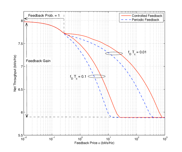
Figure 3: Net throughput versus feedback price for both the optimally controlled and periodic feedback over the perfect feedback channel. The Doppler frequency is $f_{D}=\{0.1,0.01\}/T_{c}$ and the number of transmit antenna $L=3$.

In Fig. 3, the curves of net throughput versus feedback price are plotted for both the optimally controlled feedback and the conventional periodic feedback. The net throughput for controlled and periodic feedback are maximized by value iteration [29] and a numerical search over different feedback intervals, respectively. The Doppler frequency is $f_{D}=\{0.1,0.01\}/T_{c}$ and the number of transmit antenna $L=3$. As observed from Fig. 3, the throughput for all cases decreases with the increasing feedback price. For high feedback prices, the curves flatten with net throughput fixed at $5.9$ bit/s/Hz, corresponding to no feedback. Subtracting this value from net throughput gives the feedback gain as indicated in Fig. 3. Controlled feedback is observed to increase net throughput of periodic feedback by up to $0.5$ bit/s/Hz or $24\%$ of the feedback gain of about $2.1$ bit/s/Hz. The increment in net throughput is insensitive to the change on Doppler frequency. Finally, for small feedback prices ($\alpha\leq 0.15$), both feedback algorithms perform feedback in every slot and thus all curves in Fig. 3 overlap in this range.

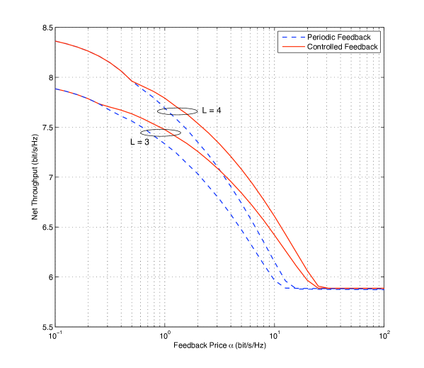
Figure 4: Net throughput versus feedback price for both the optimally controlled and periodic feedback over the perfect feedback channel. The Doppler frequency is $f_{D}=0.1/T_{c}$ and the numbers of transmit antenna $L=\{3,4\}$.

The comparison in Fig. 3 continues in Fig. 4 but for different numbers of transmit antennas $L=\{3,4\}$. It is observed that the maximum net throughput gain for controlled feedback over the periodic feedback is about $0.5$ bit/s/Hz for both $L=3$ and $L=4$. Thus this gain is insensitive to the change on $L$.

Refer to Footnote 8. The mentioned function of maximum throughput versus average feedback rate (normalized for $\alpha=1$) is plotted in Fig. 5 for $f_{D}=\{0.1,0.01\}/T_{c}$ and $L=3$. Also plotted is the matching curve for periodic feedback obtained by a numerical search over different feedback intervals. As observed from the figure, for the same average feedback rate, optimal controlled feedback provides up to $0.5$ bit/s/Hz higher throughput than periodic feedback. Alternatively, given identical throughput, the former can reduce the feedback cost by half with respect to the latter (cf. throughput $=7$ bit/s/Hz and $f_{D}T_{c}=0.01$).

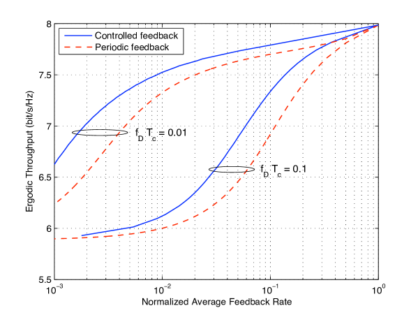
Figure 5: Throughput versus normalized average feedback rate for the optimally controlled and periodic feedback over the perfect feedback channel. The Doppler frequency is $f_{D}=\{0.1,0.01\}/T_{c}$ and the number of transmit antenna $L=3$.

Fig. 6 displays the curves of net throughput versus feedback price for the perfect and finite-rate (quantized) feedback channels. The Doppler frequency is $f_{D}=0.1/T_{c}$ and the number of transmit antennas $L=3$. The codebook used for quantizing feedback CSI has the size of $|\mathcal{F}|=16$ and is constructed using Lloyd’s algorithm [9, 8]. As observed from Fig. 4, feedback quantization reduces net throughput slightly. This loss is larger for smaller $\alpha$ (more frequent feedback) and vice versa.

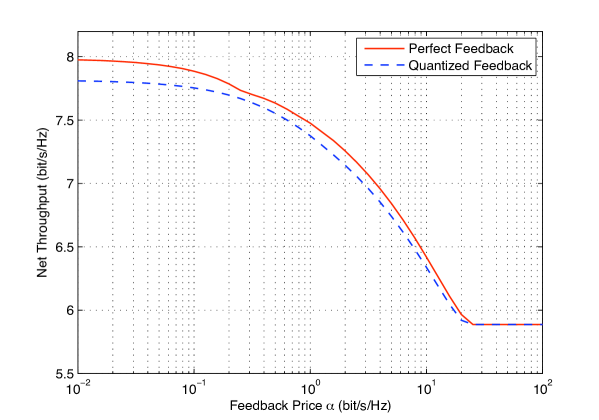
Figure 6: Net throughput versus feedback price for the optimally controlled feedback over the perfect and quantized feedback channels. The Doppler frequency is $f_{D}=0.1/T_{c}$; the number of transmit antennas $L=3$; the codebook used for quantizing feedback CSI has the size of $|\mathcal{F}|=16$.

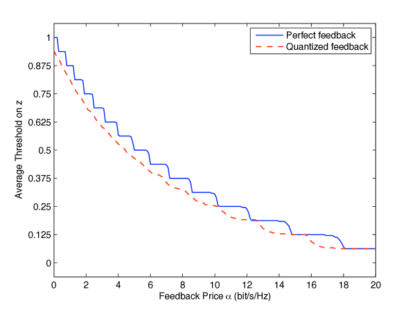
Figure 7: Average threshold on $\hat{z}$ versus feedback price $\alpha$ for the optimally controlled feedback over the perfect and quantized feedback channels. The Doppler frequency is $f_{D}=0.1/T_{c}$; the number of transmit antennas $L=3$; the codebook used for quantizing feedback CSI has the size of $|\mathcal{F}|=16$.

The optimal control policies computed in simulation using policy iteration [43] have the same threshold structure as predicted by analysis in the preceding sections. This also validates Assumption 3 on the channel temporal correlation. The thresholds for these policies are observed to be insensitive to the variation on channel gain $\hat{g}$ (cf. Remark 4) on Theorem 1). For this reason, the feedback threshold on $\hat{z}$ is averaged over the range of $\hat{g}$ and plotted against the feedback price $\alpha$ in Fig. 7, where both perfect and finite-rate feedback channels are considered. The simulation parameters follow those for Fig. 4. As observed from Fig. 7, the average feedback threshold for the perfect feedback channel is $1$ for $\alpha=0$, corresponding to feedback for every time slot; the threshold converges to zero as $\alpha$ increases. Fig. 7 shows that feedback quantization reduces the feedback threshold slightly, implying less frequent feedback. Moreover, for $\alpha=0$, the average feedback threshold for quantized feedback is smaller than one, agreeing with the remark on Corollary 2. Last, note that the humps on the curves in Fig. 7 are caused by quantizing the controller’s state space.

VII Conclusion

In this paper, we have proposed the approach of controlling feedback for maximizing net throughput of transmit beamforming systems. The optimal control policy has been proved to be of the threshold type. Under this policy, feedback is performed when the angle between transmit beamformer and the channel exceeds a threshold, which varies with the channel power. The threshold-type optimal policy has been shown to apply to both quantized and continuous controller inputs and both perfect and finite-rate feedback channels. Feedback quantization has been found to decrease net throughput similarly as increasing the feedback price. As observed from simulation results, the optimal feedback control contributes significant net throughput gains without requiring additional bandwidth or antennas.

The work opens several issues for future investigation. First, the closed-form expression of the optimal feedback control policy can be derived by making additional assumptions on channel statistics. This allows direct policy computation rather than using the more complicated policy iteration method. Second, the controlled feedback approach can be extended to other types of multi-antenna systems with feedback such as precoded spatial multiplexing or multiuser MIMO. Feedback in these systems supports multiple operations such as spatial multiplexing, interference avoidance, and scheduling. As a result, the computation and analysis of optimal control policies are more challenging than those for single-user transmit beamforming considered in this paper. Last, considering bursty data makes it necessary to jointly control the forward-link queue and CSI feedback. Addressing this issue by extending the approach in [46] can establish an optimal tradeoff relation between feedback overhead, transmission power and queueing delay.

-A Proof of Lemma 1

Let $K$ denote the height of ${\mathbf{v}}$ and ${\mathbf{A}}$. Define $\Delta v_{\ell}:=[{\mathbf{v}}]_{\ell}-[{\mathbf{v}}]_{\ell-1}$ with ${\mathbf{v}}_{-1}:=0$. Note that $\Delta v_{\ell}\geq 0$ for all $\ell$ since ${\mathbf{v}}$ is monotone. Using the above definition, we can write

$$[{\mathbf{A}}^{\dagger}{\mathbf{v}}]_{n}=\sum_{\ell=0}^{K-1}[{\mathbf{v}}]_{\ell}[{\mathbf{A}}]_{\ell,n}=\sum_{r=0}^{K-1}\sum_{\ell=r}^{K-1}\Delta v_{r}[{\mathbf{A}}]_{\ell,n}.$$ (32)

It follows that for $n_{1}\geq n_{2}$

$$[{\mathbf{A}}^{\dagger}{\mathbf{v}}]_{n_{1}}-[{\mathbf{A}}^{\dagger}{\mathbf{v}}]_{n_{2}} = \sum_{r=0}^{K-1}\Delta v_{r}\left(\sum_{\ell=r}^{K-1}[{\mathbf{A}}]_{\ell,n_{1}}-\sum_{\ell=r}^{K-1}[{\mathbf{A}}]_{\ell,n_{2}}\right)$$

$$\overset{(a)}{\geq} 0$$

where (a) follows from the monotonicity of ${\mathbf{A}}$ and that $\Delta v_{r}\geq 0\ \forall\ r$. The completes the proof of $1)$.

For $n_{1}\geq n_{2}$, the difference between the $n_{1}$th and $n_{2}$th elements of the $k$th row of ${\mathbf{B}}{\mathbf{C}}$ is

$$\sum_{\ell}[{\mathbf{B}}]_{k,\ell}[{\mathbf{C}}]_{\ell,n_{1}}-\sum_{\ell}[{\mathbf{B}}]_{k,\ell}[{\mathbf{C}}]_{\ell,n_{2}} = \sum_{\ell}[{\mathbf{B}}]_{k,\ell}([{\mathbf{C}}]_{\ell,n_{1}}-[{\mathbf{C}}]_{\ell,n_{2}})$$ (33)

$$\overset{(b)}{\geq} 0$$

where $(b)$ follows from the monotonicity of each row of ${\mathbf{C}}$ and that the elements of ${\mathbf{B}}$ are nonnegative. Then $2)$ follows from the above inequality.

-B Proof of Lemma 2

Consider fixed $m$, $n_{1}$ and $n_{2}$ with $n_{1}\geq n_{2}$ and a nonnegative function $q(m,n)$ that increases monotonically with $n$. For instance, the all-zero function is a suitable choice. Based on the value iteration in (16), to prove the lemma, it is sufficient to show that $(\mathsf{F}q)(m,n)$ is also a monotonically increasing function of $n$ given $m$. Define $\mu^{\prime}$ by

$$(\mathsf{F}q)(m,n_{2})=G(\bar{g}_{m},\bar{z}_{n_{2}},\mu^{\prime})+\beta\sum_{k,\ell}q(k,\ell)\tilde{P}_{k,m}P_{\ell,n_{2}}(\mu^{\prime}).$$

Define the matrix ${\mathbf{Q}}$ with $[{\mathbf{Q}}]_{k,\ell}=q(k,\ell)$. The above equation can be rewritten as

$$(\mathsf{F}q)(m,n_{2})=G(\bar{g}_{m},\bar{z}_{n_{2}},\mu^{\prime})+\beta[\tilde{{\mathbf{P}}}^{\dagger}{\mathbf{Q}}{\mathbf{P}}(\mu^{\prime})]_{m,n_{2}}.$$ (34)

Assume $\mu^{\prime}=1$. Then from (14) and (34)

$$(\mathsf{F}q)(m,n_{1})-(\mathsf{F}q)(m,n_{2}) \geq G(\bar{g}_{m},\bar{z}_{n_{1}},1)+\beta[\tilde{{\mathbf{P}}}^{\dagger}{\mathbf{Q}}{\mathbf{P}}(1)]_{m,n_{1}}-G(\bar{g}_{m},\bar{z}_{n_{2}},1)-\beta[\tilde{{\mathbf{P}}}^{\dagger}{\mathbf{Q}}{\mathbf{P}}(1)]_{m,n_{2}}$$

$$\overset{(a)}{=} 0$$

where $(a)$ follows from that both $G(\bar{g}_{m},\bar{z}_{n},1)$ and $P_{\ell,n}(1)$ are independent of $n$. Next, assume $\mu^{\prime}=0$. It follows that

$$(\mathsf{F}q)(m,n_{1})-(\mathsf{F}q)(m,n_{2}) \geq G(\bar{g}_{m},\bar{z}_{n_{1}},0)+\beta[\tilde{{\mathbf{P}}}^{\dagger}{\mathbf{Q}}{\mathbf{P}}(0)]_{m,n_{1}}-G(\bar{g}_{m},\bar{z}_{n_{2}},0)-\beta[\tilde{{\mathbf{P}}}^{\dagger}{\mathbf{Q}}{\mathbf{P}}(0)]_{m,n_{2}}$$ (35)

$$\overset{(b)}{\geq} \beta[\tilde{{\mathbf{P}}}^{\dagger}{\mathbf{Q}}{\mathbf{P}}(0)]_{m,n_{1}}-\beta[\tilde{{\mathbf{P}}}^{\dagger}{\mathbf{Q}}{\mathbf{P}}(0)]_{m,n_{2}}$$

$$\overset{(c)}{\geq} 0$$

where $(b)$ holds since $G(\bar{g}_{m},\bar{z}_{n},\mu^{\prime})$ is a monotonically increasing function of $\bar{z}_{n}$. $(c)$ is due to that the matrix $\tilde{{\mathbf{P}}}^{\dagger}{\mathbf{Q}}{\mathbf{P}}(0)$ has monotone rows, which results from Lemma 1 and that ${\mathbf{P}}(0)$ is monotone and ${\mathbf{Q}}$ comprises monotone rows. Combining above results proves the monotonicity of $\mathsf{F}q$ and hence $\hat{J}^{\star}_{\beta}$.

Proving the monotonicity of $\sum_{k,\ell}\hat{J}^{\star}_{\beta}(k,\ell)\tilde{P}_{k,m}P_{\ell,n}$ uses that of $\hat{J}^{\star}_{\beta}$ as shown above. The proof procedure is similar to the above steps and thus omitted.

-C Proof of Theorem 1

Consider the optimal policy $\hat{\mathcal{P}}_{\beta}^{\star}$ for maximizing the discounted reward. To simply notation, define

$$\Delta J(m,n) := \log_{2}(1+P\hat{g}_{m})-\log_{2}(1+P\hat{g}_{m}\hat{z}_{n})-\alpha+\sum_{k,\ell}\hat{J}^{\star}_{\beta}(k,\ell)\tilde{P}_{k,m}P_{\ell,n}(1)-$$ (36)

$$\sum_{k,\ell}\hat{J}^{\star}_{\beta}(k,\ell)\tilde{P}_{k,m}P_{\ell,n}(0).$$

From Bellman’s equation $\hat{J}_{\beta}^{\star}=\mathsf{F}\hat{J}_{\beta}^{\star}$ with $\mathsf{F}$ defined in (14), $\mathcal{P}^{\star}_{\beta}(\bar{g}_{m},\bar{z}_{n})=1$ if $\Delta J(m,n)>0$ or otherwise $\mathcal{P}^{\star}_{\beta}(\bar{g}_{m},\bar{z}_{n})=0$. Consider $(m_{0},n_{0})$ such that $\Delta J(m_{0},n_{0})\leq 0$. For any $n$ with $n_{0}\leq n\leq N-1$, given that $P_{\ell,n}(1)$ is independent of $n$, it follows from (36) and Lemma 2 that $\Delta J(m_{0},n)\leq 0$. Therefore for each $\hat{g}\in\hat{\mathcal{G}}$, there exists the matching $\hat{\eta}\in\hat{\mathcal{Z}}$ such that $\hat{\mathcal{P}}^{\star}_{\beta}(\hat{g},\hat{z})=0\ \forall\ \hat{z}\geq\hat{\eta}$ and $\hat{\mathcal{P}}^{\star}_{\beta}(\hat{g},\hat{z})=1\ \forall\ \hat{z}<\hat{\eta}$ if $\hat{\eta}>\bar{z}_{0}$. Defining $\hat{y}$ as the mapping from $\hat{g}$ to $\hat{\eta}$ proves that the optimal policy $\hat{\mathcal{P}}^{\star}_{\beta}$ is of the threshold type with $\hat{y}$ being the threshold function.

Next, the bounds in (29) are proved as follows. The upper bound is trivial given that $0\leq\hat{z}\leq 1$. By the above definition, $y(\hat{g})$ can be written as

$$\hat{y}(\hat{g})=\min_{\hat{z}\in\mathcal{Z}}\hat{z}\quad\textrm{s.t.}\quad\Delta J(\hat{g},\hat{z})\leq 0$$ (37)

where by abuse of notation $\Delta J(\bar{g}_{m},\bar{z}_{n}):=\Delta J(m,n)$. From(36) and Lemma 2

$$\Delta J(m,n)\geq\underbrace{\log_{2}(1+P\bar{g}_{m})-\log_{2}(1+P\bar{g}_{m}\bar{z}_{n})-\alpha}_{\Delta J^{-}(m,n)}.$$ (38)

It follows from (36) and Lemma 2 that $\Delta J(m,n)$ is a monotonically increasing function of $n$. So is $\Delta J^{-}(m,n)$ from its definition. Therefore, from (37) and (38)

$$\hat{y}(\hat{g})\geq\hat{\gamma}$$ (39)

where

$$\hat{\gamma}=\min_{\hat{z}\in\mathcal{Z}}\hat{z}\quad\textrm{s.t.}\quad\Delta J^{-}(d(\hat{g}),d(\hat{z}))\leq 0.$$ (40)

Using (39) and solving for $\hat{\gamma}$ using (40) proves that the lower bound in (29) holds for $\hat{\mathcal{P}}_{\beta}^{\star}$.

Given $0<\beta_{0}<1$, the properties for $\hat{\mathcal{P}}^{\star}_{\beta}$ as proved above hold for any $\beta\in[\beta_{0},1)$. These properties must also exist for the optimal policy giving $\hat{J}^{\star}=\lim_{\beta\rightarrow 1}(1-\beta)\hat{J}^{\star}_{\beta}$ [29]. This completes the proof.

-D Proof of Corollary 1

The first claim is obviously valid since for $\alpha=\infty$ any feedback instant causes net throughput to be $-\infty$ and thus the optimal feedback controller should block feedback by using the threshold $\hat{y}=0$. The second claim holds since for $\alpha=0$, $G(\hat{g},\hat{z},0)\leq G(\hat{g},\hat{z},1)\ \forall\ (\hat{g},\hat{z})\in\hat{X}$. Thus feedback should be performed in every time slot, corresponding to fixed $\hat{y}=1$.

-E Proof of Proposition 1

A stationary feedback policy partitions the continuous state space $\mathcal{X}$ into two sets $\mathcal{W}$ and $\mathcal{W}^{c}$ such that $\mu=1\ \forall\ (g,z)\in\mathcal{W}$ and $\mu=0\ \forall\ (g,z)\in\mathcal{W}^{c}$. To simplify notation, define $\mathcal{W}(g):=\mathcal{W}\cap(\{g\}\times\mathcal{Z})$ and $\mathcal{W}^{c}=\mathcal{W}\backslash\mathcal{W}(g)$. Moreover, let $f(z\mid\mathcal{W})$ denote the PDF of $z$ that depends on the set (policy) $\mathcal{W}$. Note that the PDF $f(g)$ of $g$ is independent of $\mathcal{W}$.

To apply Lemma 3, we design a genie-aided dummy feedback-control system similar to the current one but with a bounded continuous state space. In the virtual system, the encoder is shut down by the genie whenever $g>\tilde{g}_{M-1}$ or otherwise turned on. The average reward for this system is $I:=J(G^{\prime})$ where the reward-per-stage $G^{\prime}$ is defined in terms of $G$ in (5) as

$$G^{\prime}(g,z,\mu)=\left\{\begin{aligned} &G(g,z,\mu),&&g\geq\tilde{g}_{M-1}\\ &0,&&\textrm{otherwise}.\end{aligned}\right.$$ (41)

The maximum reward $I^{\star}$ can be written as

$$\!\!\!\!I^{\star}(M) = \!\!\!\!\!\!\max_{\mathcal{W}\in\mathcal{G}\times\mathcal{Z}}\int\limits^{\tilde{g}_{M-1}}_{0}\left\{\int\limits_{\mathcal{W}(g)}G^{\prime}(g,z,1)f(z\mid\mathcal{W})dz+\!\!\!\!\int\limits_{\mathcal{W}^{c}(g)}G^{\prime}(g,z,0)f(z\mid\mathcal{W})dz\right\}f(g)dg.$$ (42)

Next, the reward $I^{\star}(M)$ is shown to converge to $J^{\star}$ as $N$ increases. Similar to (42),

$$J^{\star} = \max_{\mathcal{W}\in\mathcal{G}\times\mathcal{Z}}\int\limits^{\infty}_{0}\left\{\int\limits_{\mathcal{W}(g)}G^{\prime}(g,z,1)f(z\mid\mathcal{W})dz+\int\limits_{\mathcal{W}^{c}(g)}G^{\prime}(g,z,0)f(z\mid\mathcal{W})dz\right\}f(g)dg$$ (43)

$$\leq \max_{\mathcal{W}\in\mathcal{G}\times\mathcal{Z}}\int\limits^{{}_{\tilde{g}_{M-1}}}_{0}\left\{\int\limits_{\mathcal{W}(g)}G^{\prime}(g,z,1)f(z\mid\mathcal{W})dz+\int\limits_{\mathcal{W}^{c}(g)}G^{\prime}(g,z,0)f(z\mid\mathcal{W})dz\right\}f(g)dg+$$

$$\max_{\mathcal{W}\in\mathcal{G}\times\mathcal{Z}}\int\limits^{\infty}_{\tilde{g}_{M-1}}\left\{\int\limits_{\mathcal{W}(g)}G^{\prime}(g,z,1)f(z\mid\mathcal{W})dz+\int\limits_{\mathcal{W}^{c}(g)}G^{\prime}(g,z,0)f(z\mid\mathcal{W})dz\right\}f(g)dg$$

$$\leq I^{\star}(M)+\max_{\mathcal{W}\in\mathcal{G}\times\mathcal{Z}}\!\!\!\!\int\limits^{\infty}_{\tilde{g}_{M-1}}\!\!\left\{\log_{2}(1+Pg)\int\limits_{\mathcal{W}(g)}\!\!\!\!f(z\mid\mathcal{W})dz+\log_{2}(1+Pg)\int\limits_{\mathcal{W}^{c}(g)}\!\!\!\!f(z\mid\mathcal{W})dz\right\}f(g)dg$$

$$= I^{\star}(M)+\int\limits^{\infty}_{\tilde{g}_{M-1}}\log_{2}(1+Pg)f(g)dg$$

$$\overset{(a)}{\leq} I^{\star}(M)+\frac{\mathbb{E}[\log_{2}(1+Pg)]}{\tilde{g}_{M-1}}$$

where $(a)$ is obtained by applying Markov’s inequality. Given that $g$ follows chi-square distribution and $\Pr(g\geq\tilde{g}_{M-1})=1/M$, $\tilde{g}_{M-1}\rightarrow\infty$ for $M\rightarrow\infty$. Therefore, since $I^{\star}$ and $\mathbb{E}[\log_{2}(1+Pg)]$ are finite, it follows form $\eqref{Eq:IJ}$ that

$$\lim_{M\rightarrow\infty}|J^{\star}-I^{\star}(M)|=0.$$ (44)

Next, consider the approximate feedback control optimization for the virtual system with a discrete state space. This space, denoted as $\hat{\mathcal{S}}$, is obtained using a quantization algorithm similar to that in Section IV-A, hence $\hat{\mathcal{S}}=(\hat{\mathcal{G}}\backslash\{\bar{g}_{M-1}\})\times\mathcal{Z}$. Let $\hat{I}^{\star}_{\beta}$ and $\hat{I}^{\star}$ denote the maximum discounted and average rewards, respectively. For the above approximated problem, the maximum quantization error is given as

$$d_{s}=\max_{0\leq m\leq M-2}\max_{0\leq n\leq N-1}\max_{\tilde{g}_{m}\leq g\leq\tilde{g}_{m+1}}\max_{\tilde{z}_{n}\leq z\leq\tilde{z}_{n+1}}\sqrt{|g-\bar{g}_{m}|^{2}+|z-\bar{z}_{n}|^{2}}.$$ (45)

Since $d_{s}\rightarrow 0$ as $M,N\rightarrow\infty$ and using the Lipschitz continuity of the conditional PDF’s of $(g,z)$ and the reward-per-stage function, it follows from Lemma 3 that

$$\lim_{M,N\rightarrow\infty}|\hat{I}^{\star}(M,N)-I^{\star}|=\lim_{\beta\rightarrow 1}\lim_{N\rightarrow\infty}(1-\beta)|\hat{I}^{\star}_{\beta}(\hat{g},\hat{z},M,N)-I^{\star}_{\beta}(g,z)|=0$$ (46)

From (44) and (46) and the triangular inequality

$$\lim_{M,N\rightarrow\infty}|J^{\star}-\hat{I}^{\star}(N)|\leq\lim_{M,N\rightarrow\infty}\left(|J^{\star}-I^{\star}(M)|+|I^{\star}-\hat{I}^{\star}(M,N)|\right)=0.$$ (47)

Furthermore, for $M,N\rightarrow\infty$, the results in Theorem 1 holds for the virtual system with the state space $\hat{\mathcal{S}}$. This completes the proof.

-F Proof of Proposition 2

Proof of the inequalities in $1)$ and $2)$: The second inequality in $1)$ holds since $G\geq G_{\epsilon}$ from their definitions in (5) and (9). In the sequel, we prove the first inequality in $1)$ based on value iteration [29]. To this end, consider two nonnegative functions $q_{1}(\hat{g},\hat{z})$ and $q_{2}(\hat{g},\hat{z})$ that have the support $\hat{\mathcal{G}}\times\hat{\mathcal{Z}}$ and monotonically increase with $\hat{z}$. Furthermore, $q_{1}(\hat{g},\hat{z})\geq q_{2}(\hat{g},\hat{z})\ \forall\ (\hat{g},\hat{z})\in\hat{\mathcal{G}}\times\hat{\mathcal{Z}}$, which is represented by $q_{1}\geq q_{2}$ for simplicity. Following the similar procedure as in the proof of Lemma 2, it can be shown that the functions $\mathsf{F}(G,{\mathbf{P}})q_{1}$ and $\mathsf{F}(G,{\mathbf{P}}_{\epsilon})q_{2}$ both monotonically increases with $\hat{z}$, where $\mathsf{F}$ is in (14).

Next, it is shown that $\mathsf{F}(G,{\mathbf{P}})q_{1}\geq\mathsf{F}(G,{\mathbf{P}}_{\epsilon})q_{2}$. Let $\mu_{a}$ and $\mu_{b}$ denote the control decisions that satisfy

$$[\mathsf{F}(G,{\mathbf{P}})q_{1}](\bar{g}_{m},\bar{z}_{n}) = G(\bar{g}_{m},\bar{z}_{n},\mu_{a})+\sum_{k,\ell}q_{1}(\bar{g}_{k},\bar{z}_{\ell})[\tilde{{\mathbf{P}}}]_{k,m}[{\mathbf{P}}(\mu_{a})]_{\ell,n}$$ (48)

$$\left[\mathsf{F}(G,{\mathbf{P}}_{\epsilon})q_{2}\right](\bar{g}_{m},\bar{z}_{n}) = G(\bar{g}_{m},\bar{z}_{n},\mu_{b})+\sum_{k,\ell}q_{2}(\bar{g}_{k},\bar{z}_{\ell})[\tilde{{\mathbf{P}}}]_{k,m}[{\mathbf{P}}_{\epsilon}(\mu_{b})]_{\ell,n}$$ (49)

If $\mu_{a}=\mu_{b}=1$,

$$[\mathsf{F}(G,{\mathbf{P}})q_{1}-\mathsf{F}(G,{\mathbf{P}}_{\epsilon})q_{2}](\bar{g}_{m},\bar{z}_{n}) = \log_{2}(1+P\bar{g}_{m})+\sum_{k,\ell}q_{1}(\bar{g}_{k},\bar{z}_{\ell})[\tilde{{\mathbf{P}}}]_{k,m}[{\mathbf{P}}(1)]_{\ell,n}$$ (50)

$$-\underset{\epsilon}{\mathbb{E}}[\log_{2}(1+P\bar{g}_{m}\epsilon)]-\sum_{k,\ell}q_{2}(\bar{g}_{k},\bar{z}_{\ell})[\tilde{{\mathbf{P}}}]_{k,m}[{\mathbf{P}}_{\epsilon}(1)]_{\ell,n}$$

$$\geq \sum_{k,\ell}q_{1}(\bar{g}_{k},\bar{z}_{\ell})[\tilde{{\mathbf{P}}}]_{k,m}[{\mathbf{P}}(1)]_{\ell,n}-\sum_{k,\ell}q_{2}(\bar{g}_{k},\bar{z}_{\ell})[\tilde{{\mathbf{P}}}]_{k,m}[{\mathbf{P}}_{\epsilon}(1)]_{\ell,n}$$

$$\overset{(a)}{\geq} \sum_{k,\ell}[\tilde{{\mathbf{P}}}]_{k,m}q_{2}(\bar{g}_{k},\bar{z}_{\ell})\left\{[{\mathbf{P}}(1)]_{\ell,n}-[{\mathbf{P}}_{\epsilon}(1)]_{\ell,n}\right\}.$$

where $(a)$ follows from $q_{1}\geq q_{2}$. For $0\leq\ell_{0}\leq N-1$ and from (12) and (30)

$$\sum_{\ell=\ell_{0}}^{N-1}[{\mathbf{P}}(1)]_{\ell,n}-\sum_{\ell=\ell_{0}}^{N-1}[{\mathbf{P}}_{\epsilon}(1)]_{\ell,n} = \int_{\hat{z}=\tilde{z}_{\ell_{0}}}^{1}\check{f}(\hat{z}\mid\hat{z}^{\prime}=1)d\hat{z}-\int_{\hat{z}=\tilde{z}_{\ell_{0}}}^{1}\underset{\epsilon}{\mathbb{E}}[\check{f}(\hat{z}\mid\hat{z}^{\prime}=\epsilon)]d\hat{z}$$

$$= \underset{\epsilon}{\mathbb{E}}\left[\int_{\hat{z}=\tilde{z}_{\ell_{0}}}^{1}\check{f}(\hat{z}\mid\hat{z}^{\prime}=1)d\hat{z}-\int_{\hat{z}=\tilde{z}_{\ell_{0}}}^{1}\check{f}(\hat{z}\mid\hat{z}^{\prime}=\epsilon)d\hat{z}\right]$$ (51)

$$\overset{(b)}{\geq} 0.$$

where $(b)$ is due to Assumption 3. Using (50) and (51) and following the similar steps as in the proof for Lemma 2 leads to that $\mathsf{F}(G,{\mathbf{P}})q_{1}\geq\mathsf{F}(G,{\mathbf{P}}_{\epsilon})q_{2}$ if $\mu_{a}=\mu_{b}=1$. If $\mu=\mu=0$, since ${\mathbf{P}}_{\epsilon}(0)={\mathbf{P}}(0)$ and $q_{1}\geq q_{2}$,

$$[\mathsf{F}(G,{\mathbf{P}})q_{1}-\mathsf{F}(G,{\mathbf{P}}_{\epsilon})q_{2}](\bar{g}_{m},\bar{z}_{n}) = \sum_{k,\ell}[q_{1}(\bar{g}_{k},\bar{z}_{\ell})-q_{2}(\bar{g}_{k},\bar{z}_{\ell})][\tilde{{\mathbf{P}}}]_{k,m}[{\mathbf{P}}(0)]_{\ell,n}$$ (52)

$$\geq 0.$$

From (14), the values of $[\mathsf{F}(G,{\mathbf{P}})q_{1}-\mathsf{F}(G,{\mathbf{P}}_{\epsilon})q_{2}]$ for $(\mu=1,\mu=0)$ and $(\mu=0,\mu=1)$ are larger than those for $(\mu=\mu=0)$ and $(\mu=\mu=1)$, respectively. Combining the above results shows that $\mathsf{F}(G,{\mathbf{P}})q_{1}\geq=\mathsf{F}(G,{\mathbf{P}}_{\epsilon})q_{2}$.

Consequently, $\hat{J}^{\star}_{\beta}(G,{\mathbf{P}})\geq\hat{J}^{\star}_{\beta}(G,{\mathbf{P}}_{\epsilon})$ since by value iteration

$$\hat{J}^{\star}_{\beta}(G,{\mathbf{P}})=\lim_{n\rightarrow\infty}\mathsf{F}^{n}(G,{\mathbf{P}})q_{1}\quad\textrm{and}\quad\hat{J}^{\star}_{\beta}(G,{\mathbf{P}}_{\epsilon})=\lim_{n\rightarrow\infty}\mathsf{F}^{n}(G,{\mathbf{P}}_{\epsilon})q_{2}.$$ (53)

As $\hat{J}^{\star}=\lim_{\beta\rightarrow 1}(1-\beta)\hat{J}^{\star}_{\beta}$, the first inequality in 1) of the proposition statement is proved.

The inequalities in $2)$ of the proposition statement can be proved also using the above procedure.

Proof of the inequalities in $3)$ and $4)$: The inequalities in $3)$ and $4)$ can be proved using similar procedures. Thus we focus on proving that in $3)$. The reward-per-stage function in (9) can lower bounded below, where the fourth argument is the weighted feedback price

$$G_{\epsilon}(\hat{g},\hat{z},1,\alpha) = \underset{\epsilon}{\mathbb{E}}\left[\log_{2}\left(1/\epsilon+P\hat{g}\right)\right]+\underset{\epsilon}{\mathbb{E}}[\log_{2}\epsilon]-\alpha$$ (54)

$$\overset{(a)}{\geq} \log_{2}\left(1+P\hat{g}\right)+\underset{\epsilon}{\mathbb{E}}[\log_{2}\epsilon]-\alpha$$

$$= G(\hat{g},\hat{z},1,\alpha-\underset{\epsilon}{\mathbb{E}}[\log_{2}\epsilon])$$

where $(a)$ uses $\delta\leq 1$. Combining (54) and $G_{\epsilon}(\hat{g},\hat{z},0)=G(\hat{g},\hat{z},0)$ gives the desired result.

References

- [1] A. Paulraj, R. Nabar, and D. Gore, Introduction to Space-Time Wireless Communications. Cambridge University Press, 2003.
- [2] D. J. Love, R. W. Heath Jr., W. Santipach, and M. L. Honig, “What is the value of limited feedback for MIMO channels?,” IEEE Communications Magazine, vol. 42, pp. 54–59, Oct. 2004.
- [3] D. J. Love, R. W. Heath, V. K. N. Lau, D. Gesbert, B. D. Rao, and M. Andrews, “An overview of limited feedback in wireless communication systems,” IEEE Journal on Sel. Areas in Communications, vol. 26, no. 8, pp. 1341–1365, 2008.
- [4] D. J. Love, R. W. Heath Jr., and T. Strohmer, “Grassmannian beamforming for multiple-input multiple-output wireless systems,” IEEE Trans. on Inform. Theory, vol. 49, pp. 2735–2747, Oct. 2003.
- [5] K. K. Mukkavilli, A. Sabharwal, E. Erkip, and B. Aazhang, “On beamforming with finite rate feedback in multiple antenna systems,” IEEE Trans. on Inform. Theory, vol. 49, pp. 2562–79, Oct. 2003.
- [6] J. C. Roh and B. D. Rao, “Efficient feedback methods for MIMO channels based on parameterization,” IEEE Trans. on Wireless Communications, vol. 6, pp. 282–292, Jan. 2007.
- [7] J. Choi, B. Mondal, and R. W. H. Jr., “Interpolation based unitary precoding for spatial multiplexing MIMO-OFDM with limited feedback,” IEEE Trans. on Sig. Proc., vol. 54, pp. 4730–4740, Dec. 2006.
- [8] P. Xia, S. Zhou, and G. B. Giannakis, “Achieving the Welch bound with difference sets,” IEEE Trans. on Inform. Theory, vol. 51, pp. 1900–1907, May 2005.
- [9] V. K. N. Lau, Y. Liu, and T.-A. Chen, “On the design of MIMO block-fading channels with feedback-link capacity constraint,” IEEE Trans. on Communications, vol. 52, pp. 62–70, Jan. 2004.
- [10] D. J. Love and R. W. Heath Jr., “Limited feedback unitary precoding for orthogonal space-time block codes,” IEEE Trans. on Sig. Proc., vol. 53, pp. 64–73, Jan. 2005.
- [11] D. J. Love and R. W. Heath Jr., “Limited feedback unitary precoding for spatial multiplexing systems,” IEEE Trans. on Inform. Theory, vol. 51, pp. 1967–1976, Aug. 2005.
- [12] D. Gesbert, M. Kountouris, R. W. Heath Jr., C.-B. Chae, and T. Salzer, “From single user to multiuser communications: Shifting the MIMO paradigm,” IEEE Signal Processing Magazine, vol. 24, no. 5, pp. 36–46, 2007.
- [13] “IEEE 802.16 Task Group 3.” http://grouper.ieee.org/groups/802/16/tg3/.
- [14] “3GPP TR 25.814: Physical layer aspects for evolved universal terrestrial radio access (release 7),” Online: http://www.3gpp.org/, 2006.
- [15] B. C. Banister and J. R. Zeidler, “Feedback assisted transmission subspace tracking for MIMO systems,” IEEE Journal on Sel. Areas in Communications, vol. 21, pp. 452–463, March 2003.
- [16] K. Huang, R. W. Heath, and J. G. Andrews, “Limited feedback beamforming over temporally-correlated channels,” IEEE Trans. on Sig. Proc., vol. 57, pp. 1959–1975, May 2009.
- [17] R. Knopp and P. Humblet, “Information capacity and power control in single-cell multiuser communications,” in Proc., IEEE Intl. Conf. on Communications, vol. 1, pp. 331–5, 1995.
- [18] P. Viswanath, D. Tse, and R. Laroia, “Opportunistic beamforming using dumb antennas,” IEEE Trans. on Inform. Theory, vol. 48, pp. 1277–1294, June 2002.
- [19] T. Tang and R. W. Heath, Jr., “Opportunistic feedback for downlink multiuser diversity,” IEEE Commun. Lett., vol. 9, pp. 948–950, Oct. 2005.
- [20] T. Tang, R. W. Heath Jr., S. Cho, and S. Yun, “Opportunistic feedback for multiuser MIMO systems with linear receivers,” IEEE Trans. on Communications, vol. 55, pp. 1020–1032, May 2007.
- [21] S. Sanayei and A. Nosratinia, “Opportunistic beamforming with limited feedback,” in Proc., IEEE Asilomar, pp. 648–652, Nov. 2005.
- [22] K.-B. Huang, R. W. Heath Jr., and J. G. Andrews, “SDMA with a sum feedback rate constraint,” IEEE Trans. on Sig. Proc., vol. 55, pp. 3879–91, July 2007.
- [23] C. Swannack, G. W. Wornell, and E. Uysal-Biyikoglu, “MIMO broadcast scheduling with quantized channel state information,” in Proc., IEEE Intl. Symposium on Information Theory, pp. 1788–92, July 2006.
- [24] S. Sanayei and A. Nosratinia, “Exploiting multiuser diversity with only 1-bit feedback,” in Proc., IEEE Wireless Communications and Networking Conf., vol. 2, pp. 978–983, 2005.
- [25] D. J. Love, “Duplex distortion models for limited feedback mimo communication,” IEEE Trans. on Sig. Proc., vol. 54, pp. 766–774, Feb. 2006.
- [26] C. K. Au-Yeung and D. J. Love, “Optimization and tradeoff analysis of two-way limited feedback beamforming systems,” IEEE Trans. on Wireless Communications, vol. 8, pp. 2570–2579, May 2009.
- [27] Y. Xie, C. N. Georghiades, and K. Rohani, “Optimal bandwidth allocation for the data and feedback channels in MISO-FDD systems,” IEEE Trans. Commun, vol. 54, pp. 197–203, Feb. 2006.
- [28] V. Bawa, “Optimal rules for ordering uncertain prospects,” Journal of Financial Economics, vol. 2, pp. 95–121, Feb. 1975.
- [29] D. P. Bertseka, Dynamic Programming and Optimal Control (Vol. I and II). Athena Scientific, 3rd ed., 2007.
- [30] H. Wang and N. Moayeri, “Finite-state Markov channel – a useful model for radio communication channels,” IEEE Trans. on Veh. Technology, vol. 44, pp. 163–71, Feb. 1995.
- [31] C. Pimentel, T. H. Falk, and L. Lisboa, “Finite-state Markov modeling of correlated Rician-fading channels,” IEEE Trans. on Veh. Technology, vol. 53, pp. 1491–1501, Sept. 2004.
- [32] Q. Zhang and S. A. Kassam, “Finite-state Markov model for Rayleigh fading channels,” IEEE Trans. on Communications, vol. 47, pp. 1688–1692, Nov. 1999.
- [33] P. Ivanis, D. Drajic, and B. Vucetic, “Performance evaluation of adaptive MIMO-MRC systems with imperfect CSI by a Markov model,” in Proc., IEEE Veh. Technology Conf., pp. 1496–1500, Apr. 2007.
- [34] P.-H. Kuo, P. J. Smith, and L. M. Garth, “A Markov model for MIMO channel condition number with application to dual-mode antenna selection,” in Proc., IEEE Veh. Technology Conf., pp. 471–475, Apr. 2007.
- [35] P. Sadeghi and P. Rapajic, “Capacity analysis for finite-state Markov mapping of flat-fading channels,” IEEE Trans. on Communications, vol. 53, pp. 833–840, May 2005.
- [36] R. C. Daniels, K. Mandke, K. Truong, S. Nettles, and R. W. H. Jr., “Throughput and delay measurements of limited feedback beamforming for indoor wireless networks,” in Proc., IEEE Globecom, Nov. 2008.
- [37] V. Tarokh, H. Jafarkhani, and A. R. Calderbank, “Space-time block codes from orthogonal designs,” IEEE Trans. on Inform. Theory, vol. 45, pp. 1456–1467, Jul. 1999.
- [38] I. E. Telatar, “Capacity of multi-antenna Gaussian channels,” European Trans. on Telecomm., vol. 10, pp. 585–595, June 1999.
- [39] T. K. Y. Lo, “Maximum ratio transmission,” IEEE Trans. on Communications, vol. 47, pp. 1458–61, Oct. 1999.
- [40] C. K. Au-Yeung and D. J. Love, “On the performance of random vector quantization limited feedback beamforming in a MISO system,” IEEE Trans. on Wireless Communications, vol. 6, pp. 458–462, Feb. 2007.
- [41] Y. Sawaragi, H. Nakayama, and T. Tanino, Theory of multiobjective optimization. Academic Press, 1985.
- [42] N. Jindal, “MIMO broadcast channels with finite-rate feedback,” IEEE Trans. on Inform. Theory, vol. 52, pp. 5045–5060, Nov. 2006.
- [43] D. Bertsekas, “Convergence of discretization procedures in dynamic programming,” IEEE Trans. on Automatic Control, vol. 20, pp. 415–419, Mar. 1975.
- [44] R. Gallager, Discrete Stochastic Processes. Springer, 1995.
- [45] R. H. Clarke, “A statistical theory of mobile radio reception,” Bell Syst. Tech. J., pp. 957–1000, 1974.
- [46] R. A. Berry and R. G. Gallager, “Communication over fading channels with delay constraints,” IEEE Trans. on Inform. Theory, vol. 48, pp. 1135–1149, May 2002.