ABSTRACT

In this paper, we investigate the new agegraphic dark energy model in the framework of Brans-Dicke theory which is a natural extension of the Einstein’s general relativity. In this framework the form of the new agegraphic dark energy density takes as $\rho_{q}=3n^{2}\Phi(t)\eta^{-2}$, where $\eta$ is the conformal age of the universe and $\Phi(t)$ is the Brans-Dicke scalar field representing the inverse of the time-variable Newton’s constant. We derive the equation of state of the new agegraphic dark energy and the deceleration parameter of the universe in the Brans-Dicke theory. It is very interesting to find that in the Brans-Dicke theory the agegraphic dark energy realizes quintom-like behavior, i.e., its equation of state crosses the phantom divide $w=-1$ during the evolution. We also compare the situation of the agegraphic dark energy model in the Brans-Dicke theory with that in the Einstein’s theory. In addition, we discuss the new agegraphic dark energy model with interaction in the framework of the Brans-Dicke theory.

1 Introduction

There is no denying that our universe is currently undergoing a period of accelerated expansion, and consequently the investigation of dark energy has become one of the hottest topics in modern cosmology. This cosmic acceleration has been widely proved by many astronomical observations, especially by the observation of the type Ia supernovae [1] which provides confirmatory evidence for this remarkable finding. Combining the analysis of cosmological observations we realize that the universe is spatially flat and a mysterious dominant component, dark energy, which is an exotic matter with large enough negative pressure, leads to this cosmic acceleration. The preferred candidate of dark energy is the Einstein’s cosmological costant which can fit the observations well, but is plagued by the “fine-tuning” and the “cosmic coincidence” problems [2]. In order to alleviate the cosmological-constant problems and explain the acceleration expansion, many dynamical dark energy models have been proposed, such as quintessence [3], phtantom [4], quintom [5], $k$-essence [6], hessence [7], tachyon [8], Chaplygin gas [9], Yang-Mills condensate [10], ect.

In fact, the dark energy problem might be in essence an issue of quantum gravity [11]. By far, however, a complete theory of quantum gravity has not been established, so it seems that we have to consider the effects of gravity in some effective quantum field theory in which some fundamental principles of quantum gravity should be taken into account. It should be stressed that the holographic principle [12] is commonly believed as a fundamental principle of the underlying quantum gravity theory. Based on the holographic principle, a viable holographic dark energy model was constructed by Li [13] by choosing the scale of the future event horizon of the universe as the infrared cutoff of the effective quantum field theory. The holographic dark energy model is very successful in explaining the observational data and has been studied widely (see, e.g., Refs. [14, 15, 16]). More recently, a new dark energy model, dubbed “agegraphic dark energy” model, has been proposed by Cai [17], which is also related to the holographic principle of quantum gravity. The agegraphic dark energy takes into account the uncertainty relation of quantum mechanics together with the gravitational effect in general relativity.

In the general relativity, one can measure the spacetime without any limit of accuracy. However, in the quantum mechanics, the well-known Heisenberg uncertainty relation puts a limit of accuracy in these measurements. Following the line of quantum fluctuations of spacetime, Károlyházy and his collaborators [18] (see also Ref. [19]) made an interesting observation concerning the distance measurement for Minkowski spacetime through a light-clock Gedanken experiment, namely, the distance $t$ in Minkowski spacetime cannot be known to a better accuracy than

$$\delta t=\lambda t_{p}^{2/3}t^{1/3}~{},$$ (1.1)

where $\lambda$ is a dimensionless constant of order unity.

The Károlyházy relation (1.1) together with the time-energy uncertainty relation enables one to estimate a quantum energy density of the metric fluctuations of Minkowski spacetime [19, 20]. Following Refs. [19, 20], with respect to the Eq. (1.1) a length scale $t$ can be known with a maximum precision $\delta t$ determining thereby a minimal detectable cell $\delta t^{3}\sim t_{p}^{2}t$ over a spatial region $t^{3}$. Such a cell represents a minimal detectable unit of spacetime over a given length scale $t$. If the age of the Minkowski spacetime is $t$, then over a spatial region with linear size $t$ (determining the maximal observable patch) there exists a minimal cell $\delta t^{3}$ the energy of which due to time-energy uncertainty relation cannot be smaller than [19, 20]

$$E_{\delta t^{3}}\sim t^{-1}~{}.$$ (1.2)

Therefore, the energy density of metric fluctuations of Minkowski spacetime is given by [19, 20]

$$\rho_{q}\sim\frac{E_{\delta t^{3}}}{\delta t^{3}}\sim\frac{1}{t_{p}^{2}t^{2}}\sim\frac{M_{p}^{2}}{t^{2}}~{},$$ (1.3)

where $M_{p}$ is the reduced Planck mass. This energy density can be viewed as the density of dark energy (i.e., the agegraphic dark energy). Thus, furthermore, the energy density of the agegraphic dark energy can be written as [17]

$$\rho_{q}=3n^{2}M^{2}_{p}t^{-2},$$ (1.4)

where the numerical factor $3n^{2}$ is introduced to parameterize some uncertainties, such as the species of quantum fields in the universe, the effect of curved spacetime (since the energy density is derived for Minkowski spacetime) and so on.

In the original version of the agegraphic dark energy model [17], the time scale $t$ in Eq. (1.4) is chosen to be the age of the universe $T$, however, unfortunately this version suffers from some internal inconsistencies of the model [21, 22]. To avoid these internal inconsistencies, a new version of this model was proposed by Wei and Cai [22] by replacing the cosmic age $T$ with the cosmic conformal age $\eta$ for the time scale in Eq. (1.4). So, the new agegraphic dark energy has the energy density [22]

$$\rho_{q}=3n^{2}M^{2}_{p}\eta^{-2},$$ (1.5)

where

$$\eta\equiv\int_{0}^{t}\frac{dt}{a}=\int_{0}^{a}\frac{da}{a^{2}H}$$ (1.6)

is the conformal age of the universe. The new agegraphic dark energy model is successful in fitting the observational data and has been studied extensively [23, 24, 25]. In this note, we will study the new agegraphic dark energy model in the framework of the Brans-Dicke theory.

The Brans-Dicke theory [26] is a natural alternative and a simple extension of the Einstein’s general relativity theory. Also, it is the simplest example of a scalar-tensor theory of gravity [27]. In the Brans-Dicke theory, the purely metric coupling of matter with gravity is preserved, thus the universality of free fall (equivalence principle) and the constancy of all non-gravitational constants are ensured. The Brans-Dicke theory can pass the experimental tests from the solar system [28] and provide an explanation of the accelerated expansion of the universe [29]. Recently, Wu et al. [30, 31] developed the covariant cosmological perturbation formalism in the case of Brans-Dicke gravity, and applied this method to the calculation of cosmic microwave background anisotropy and large scale structures. Furthermore, they derived observational constraint on the Brans-Dicke theory in a flat Friedmann-Robertson-Walker (FRW) universe with the latest Wilkinson Microwave Anisotropy Probe (WMAP) and Sloan Digital Sky Survey (SDSS) data [31]. In the Brans-Dicke theory, the gravitational constant is replaced with the inverse of a time-dependent scalar field, namely, $\Phi(t)=\frac{1}{8\pi G}$, and this scalar field couples to gravity with a coupling $\omega$.

Since the Brans-Dicke theory is an alternative to the general relativity and evokes wide interests in the modern cosmology, it is worthwhile to discuss dark energy models in this framework. Recently, the holographic dark energy model has been studied in the framework of the Brans-Dicke theory [32] (for the case of the holographic Ricci dark energy, see [33]). In this work, we consider the agegraphic dark energy model in the Brans-Dicke theory. We are interested in how the agegraphic dark energy evolves in the universe in the framework of Brans-Dicke theory.

This paper is organized as follows: In Sec. 2, we briefly review the Friedmann equation in the Brans-Dicke theory. We study the original agegraphic dark energy and the new agegraphic dark energy in Brans-Dicke theory in Secs. 3 and 4, respectively. In Sec. 5, we further discuss the new agegraphic dark energy with interaction. In Sec. 6, we give the conclusion.

2 Friedmann Equation in Brans-Dicke Theory

First, we will briefly review the Friedmann equation of the Brans-Dicke cosmology. In the Jordan frame, the action for the Brans-Dicke theory with matter fields is written as

$$S=\int d^{4}x\sqrt{g}\left[\frac{1}{2}\left(\Phi R-\omega\frac{\nabla_{\mu}\Phi\nabla^{\mu}\Phi}{\Phi}\right)+\mathcal{L}_{M}\right]$$ (2.1)

where $\Phi$ is the Brans-Dicke scalar field, $\omega$ is the generic dimensionless parameter of the Brans-Dicke theory, and ${\cal L}_{M}$ is the Lagrangian of matter fields. In the Jordan frame, the matter minimally couples to the metric and there is no interaction between the scalar field $\Phi$ and the matter fields. The equations of motion for the metric $g_{\mu\nu}$ and the Brans-Dicke scalar field $\Phi$ are

$$\begin{split}G_{\mu\nu}=R_{\mu\nu}-{1\over 2}g_{\mu\nu}R&=\frac{1}{\Phi}T^{M}_{\mu\nu}+T^{BD}_{\mu\nu},\\ \nabla_{\mu}\nabla^{\mu}\Phi&=\frac{1}{2\omega+3}T^{M\mu}_{\quad\mu},\end{split}$$ (2.2)

where $T^{M}_{\mu\nu}=(2/\sqrt{g})\delta(\sqrt{g}\mathcal{L}_{M})/\delta g^{\mu\nu}$ is the energy-momentum tensor for the matter fields defined as usual, and in cosmology it can be expressed as the form of perfect fluid

$$T^{M}_{\mu\nu}=(\rho_{M}+p_{M})U_{\mu}U_{\nu}+p_{M}g_{\mu\nu},$$ (2.3)

where $\rho_{M}$ and $p_{M}$ denote the energy density and pressure of the matter, respectively, and $U_{\mu}$ is the four velocity vector normalized as $U_{\mu}U^{\mu}=-1$. The energy-momentum tensor of the Brans-Dicke scalar field $\Phi$ is expressed as

$$T^{BD}_{\mu\nu}=\frac{\omega}{\Phi^{2}}\left(\nabla_{\mu}\Phi\nabla_{\nu}\Phi-{1\over 2}g_{\mu\nu}\nabla_{\alpha}\Phi\nabla^{\alpha}\Phi\right)+\left(\nabla_{\mu}\nabla_{\nu}\Phi-g_{\mu\nu}\nabla_{\alpha}\nabla^{\alpha}\Phi\right)$$ (2.4)

Note that in the $\omega\rightarrow\infty$ limit of the Brans-Dicke theory, the Einstein’s general relativity will be recovered.

Consider now a spatially flat FRW universe containing matter component and agegraphic dark energy. For simplicity, we also assume that the Brans-Dicke scalar field is only a time-dependent function, namely, $\Phi=\Phi(t)$. We can get the equations describing the background evolution

$$H^{2}+H\frac{\dot{\Phi}}{\Phi}-\frac{\omega}{6}\frac{\dot{\Phi}^{2}}{\Phi^{2}}=\frac{\rho_{m}+\rho_{q}}{3\Phi},$$ (2.5)

$$2\frac{\ddot{a}}{a}+H^{2}+\frac{\omega}{2}\frac{\dot{\Phi}^{2}}{\Phi^{2}}+2H\frac{\dot{\Phi}}{\Phi}+\frac{\ddot{\Phi}}{\Phi}=-\frac{p_{q}}{\Phi},$$ (2.6)

where $H={\dot{a}/a}$ is the Hubble parameter, a dot denotes the derivative with respect to the cosmic time, $\rho_{m}$ is matter density, $\rho_{q}$ is the density of agegraphic dark energy and $p_{q}$ is the pressure of agegraphic dark energy. Assuming $\Phi(t)=\Phi_{0}a(t)^{\alpha}$ (here we have taken $a_{0}=1$, where the subscript $0$ denotes the present day), the Friedmann equation (2.5) becomes

$$H^{2}(1+\alpha-\frac{\omega\alpha^{2}}{6})=\frac{\rho_{m}+\rho_{q}}{3\Phi}.$$ (2.7)

It is easy to see from the Friedmann equation (2.7) in Brans-Dicke theory that in the limit of $\alpha\rightarrow 0$ the standard cosmology will be recovered.

3 The Old Version: Age of the Universe as Time Scale

We shall first consider the old version of the agegraphic dark energy model. In this version, the time scale is chosen as the age of the universe,

$$T=\int_{0}^{a}\frac{da}{aH},$$ (3.1)

so in the Brans-Dicke theory the energy density of the agegraphic dark energy is given by

$$\rho_{q}=3n^{2}\Phi(t)T^{-2}.$$ (3.2)

The Friedmann (2.7) can be rewritten as

$$H^{2}=H^{2}_{0}\Omega_{m0}a^{-(3+\alpha)}+\Omega_{q}H^{2},$$ (3.3)

where $\Omega_{m0}=\frac{2}{(6+6\alpha-\omega\alpha^{2})}\frac{\rho_{m0}}{\Phi_{0}H^{2}_{0}}$ and

$$\Omega_{q}=\frac{2}{6+6\alpha-\omega\alpha^{2}}\frac{1}{\Phi}\frac{\rho_{q}}{H^{2}}=\tilde{n}_{0}\frac{1}{H^{2}T^{2}}$$ (3.4)

with $\tilde{n}_{0}=\frac{6n^{2}}{6+6\alpha-\omega\alpha^{2}}$. Using Eqs. (3.1) and (3.4), we get

$$\int_{0}^{a}\frac{da}{aH}=\frac{1}{H}\sqrt{\frac{\tilde{n}_{0}}{\Omega_{q}}}.$$ (3.5)

From Eq. (3.3), we obtain

$$\frac{1}{H}=\sqrt{a^{(3+\alpha)}(1-\Omega_{q})}\frac{1}{H_{0}\sqrt{\tilde{n}_{0}}}.$$ (3.6)

Considering Eqs. (3.5) and (3.6), we obtain the eqution of motion for $\Omega_{q}$ as

$$\Omega_{q}^{\prime}=\Omega_{q}\left(1-\Omega_{q}\right)\left(3+\alpha-\frac{2}{\sqrt{\tilde{n}_{0}}}\sqrt{\Omega_{q}}\right),$$ (3.7)

where the prime denotes the derivative with respect to $\ln a$. The energy conservation equation $\dot{\rho}_{q}+3H(1+w_{q})\rho_{q}=0$ leads to

$$w_{q}=-1-\frac{1}{3}\frac{d\ln\rho_{q}}{d\ln a}.$$ (3.8)

Using Eqs. (3.7), (3.8) and $\rho_{q}=\frac{\Omega_{q}}{1-\Omega_{q}}\rho_{m0}a^{-3}$, we get the equation of state of the old agegraphic dark energy

$$w_{q}=-\frac{1}{3}\left(3+\alpha-\frac{2}{\sqrt{\tilde{n}_{0}}}\sqrt{\Omega_{q}}\right).$$ (3.9)

Now let us consider the current value of the Brans-Dicke scalar field $\Phi$. We naturally have $\Phi_{0}=1/8\pi G$ today, and obviously we can let $\Omega_{m0}=\frac{2}{(6+6\alpha-\omega\alpha^{2})}\frac{\rho_{m0}}{\Phi_{0}H^{2}_{0}}\equiv\frac{8\pi G\rho_{m0}}{3H_{0}^{2}}$. Thus, the relations $\omega\alpha=6$ and $\tilde{n}_{0}=n^{2}$ are derived. This leads to Eqs. (3.7) and (3.9) rewritten as

$$\Omega_{q}^{\prime}=\Omega_{q}\left(1-\Omega_{q}\right)\left(3+\alpha-\frac{2}{n}\sqrt{\Omega_{q}}\right),$$ (3.10)

$$w_{q}=-\frac{1}{3}\left(3+\alpha-\frac{2}{n}\sqrt{\Omega_{q}}\right).$$ (3.11)

Also, we can obtain the deceleration parameter

$$q=-\frac{\ddot{a}}{aH^{2}}=\frac{3w_{q}\Omega_{q}+1+4\alpha+\alpha^{2}}{2+\alpha}.$$ (3.12)

The solar-system experiments give the result for the value of $\omega$ is $|\omega|>40000$ [28]. However, when probing the larger scales, the limit obtained will be weaker than this result. In Ref. [34], the authors found that $\omega$ is smaller than 40000 on a cosmological scale. Specifically, Wu and Chen [31] obtained the observational constraint on the Brans-Dicke model in a flat universe with cosmological constant and cold dark matter using the latest WMAP and SDSS data. They found that within 2$\sigma$ range, the value of $\omega$ satisfies $\omega<-120.0$ or $\omega>97.8$ [31]. They also obtained the constraint on the rate of change of G at present [31],

$$-1.75\times 10^{-12}{\rm yr}^{-1}<\frac{\dot{G}}{G}<1.05\times 10^{-12}{\rm yr}^{-1}$$ (3.13)

at $2\sigma$ confidence level. So in our case we get

$$\left|\frac{\dot{G}}{G}\right|=\left|\frac{\dot{\Phi}}{\Phi}\right|=\alpha H<10^{-12}{\rm yr}^{-1},$$ (3.14)

and it implies

$$\alpha<\frac{1}{H}\times 10^{-12}{\rm yr}^{-1}.$$ (3.15)

Note that we only consider the positive sector of $\omega$. Taking the current value of the Hubble constant $h\simeq 0.7$ into account, one can estimate the bounds on $\alpha$,

$$\alpha<0.01.$$ (3.16)

Note also that in Ref. [35] Xu, Lu and Li have performed observational constraints on the holographic dark energy model in Brans-Dicke theory and they found that the 1$\sigma$ bound on $\alpha$ is $\alpha<0.14$.

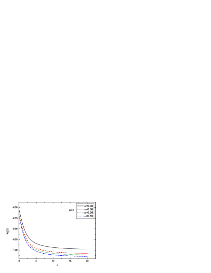
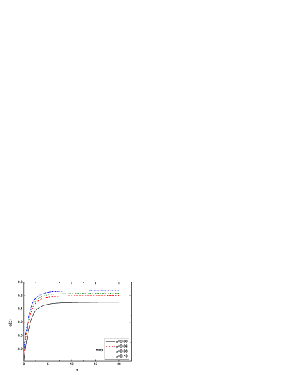
Figure 1: The old agegraphic dark energy model in Brans-Dicke theory: the equation of state of dark energy $w_{q}(z)$ and the deceleration parameter of the universe $q(z)$. In this figure, we fix $n=3$ and vary $\alpha$ to compare the usual case with the Brans-Dicke ones. We take $\Omega_{q0}=0.72$.

Figure 1 shows the equation of state of dark energy $w_{q}(z)$ and the deceleration parameter of the universe $q(z)$ in the old agegraphic dark energy model within the framework of Brans-Dicke theory. To compare the usual case ($\alpha=0$) with the Brans-Dicke ones ($\alpha\neq 0$), we fix $n=3$ and vary $\alpha$ in this figure. Note that to make a clear comparison we choose some large values for $\alpha$. Recall that in the usual case the old agegrahic dark energy behaves like a thawing quintessence [23]. However, in the Brans-Dicke theory, the equation of state of the old agegraphic dark energy can cross the cosmological-constant boundary $w=-1$ (“phantom divide”), realizing the quintom behavior. This can be clearly seen from Eq. (3.11).

4 The New Version: Conformal Age of the Universe as Time Scale

We now consider the new version of the agegraphic dark energy model with the dark energy density

$$\rho_{q}=3n^{2}\Phi(t)\eta^{-2},$$ (4.1)

where $\eta$ is the conformal age of the universe given by Eq. (1.6).

The Friedmann equation (2.7) can be rewritten as

$$H^{2}=H^{2}_{0}\Omega_{m0}a^{-(3+\alpha)}+\Omega_{q}H^{2},$$ (4.2)

where

$$\Omega_{q}=\frac{2}{6+6\alpha-\omega\alpha^{2}}\frac{1}{\Phi}\frac{\rho_{q}}{H^{2}}=\tilde{n}_{0}\frac{1}{H^{2}\eta^{2}}.$$ (4.3)

Combining Eqs. (1.6) and (4.3), we obtain

$$\int\frac{da}{a^{2}H}=\frac{1}{H}\sqrt{\frac{\tilde{n_{0}}}{\Omega_{q}}}.$$ (4.4)

Considering Eqs. (4.4) and (4.2), we also obtain the equation of motion for $\Omega_{q}$,

$$\Omega_{q}^{\prime}=\Omega_{q}\left(1-\Omega_{q}\right)\left(3+\alpha-\frac{2}{a\sqrt{\tilde{n}_{0}}}\sqrt{\Omega_{q}}\right).$$ (4.5)

Furthermore, linking the conversation equation of dark energy with $\rho_{q}=\frac{\Omega_{q}}{1-\Omega_{q}}\rho_{m0}a^{-3}$ gives rise to

$$w_{q}=-\frac{1}{3}\left(3+\alpha-\frac{2}{a\sqrt{\tilde{n}_{0}}}\sqrt{\Omega_{q}}\right).$$ (4.6)

As discussed above, we have the relations $\omega\alpha=6$ and $\tilde{n}_{0}=n^{2}$, so Eqs. (4.5) and (4.6) are rewritten as

$$\Omega_{q}^{\prime}=\Omega_{q}\left(1-\Omega_{q}\right)\left(3+\alpha-\frac{2}{an}\sqrt{\Omega_{q}}\right),$$ (4.7)

$$w_{q}=-\frac{1}{3}\left(3+\alpha-\frac{2}{na}\sqrt{\Omega_{q}}\right).$$ (4.8)

Obviously, the above two equations can also be rewritten as

$$\frac{d\Omega_{q}}{dz}=-\Omega_{q}\left(1-\Omega_{q}\right)\left[(3+\alpha)\frac{1}{1+z}-\frac{2}{n}\sqrt{\Omega_{q}}\right],$$ (4.9)

$$w_{q}=-\frac{1}{3}\left[(3+\alpha)-\frac{2}{n}\sqrt{\Omega_{q}}(1+z)\right].$$ (4.10)

When considering the range of the fractional dark energy density $0\leq\Omega_{q}\leq 1$, one can see from Eq. (4.10) that the equation of state of the new agegraphic dark energy is in the range

$$-\frac{1}{3}\left(3+\alpha\right)<w_{q}<-\frac{1}{3}\left(3+\alpha-\frac{2}{n}(1+z)\right),$$ (4.11)

so it is obvious that in the Brans-Dicke gravity case the new agegraphic dark energy can realize the quintom behavior, i.e., the equation of state of dark energy can cross $-1$ during the evolution. The deceleration parameter $q$ in this case has the same form as Eq. (3.12).

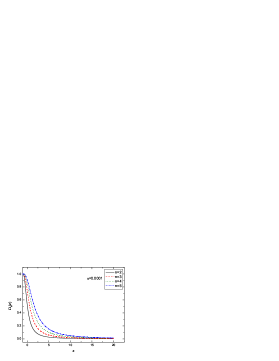
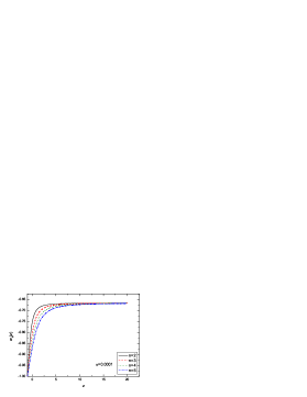
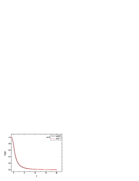
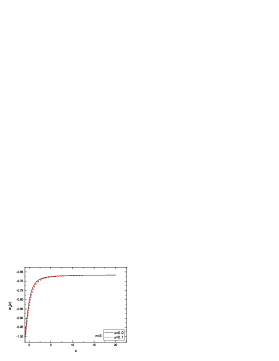
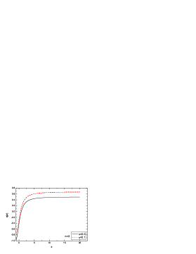
Figure 2: The new agegraphic dark energy model in Brans-Dicke theory: the fractional dark energy density $\Omega_{q}(z)$, the equation of state of dark energy $w_{q}(z)$ and the deceleration parameter of the universe $q(z)$. Here we use the initial condition $\Omega_{q}(z_{ini})=\frac{n^{2}(1+\alpha)^{2}}{4(1+z_{ini})^{2}}$ at $z_{ini}=2000$. In this figure, we first fix $\alpha=0.0001$ and compare the cases with different $n$, and then we fix $n=3$ and compare the usual case ($\alpha=0$) with the Brans-Dicke one ($\alpha\neq 0$).

To illustrate the new agegraphic dark energy model in Brans-Dicke cosmology, we plot the fractional dark energy density $\Omega_{q}(z)$, the equation of state of dark energy $w_{q}(z)$ and the deceleration parameter of the universe $q(z)$ in Fig. 2. The initial condition in this case is $\Omega_{q}(z_{ini})=\frac{n^{2}(1+\alpha)^{2}}{4(1+z_{ini})^{2}}$ at some large enough $z_{ini}$, and we choose $z_{ini}=2000$ following Ref. [22]. So, in the case of Brans-Dicke cosmology, the dynamical behavior of the agegraphic dark energy is determined by the parameters $n$ and $\alpha$. We first fix $\alpha=0.0001$ and compare the cases with different $n$, see the upper three panels of Fig. 2. Next, we fix $n=3$ and compare the usual case ($\alpha=0$) with the Brans-Dicke one ($\alpha=0.1$), see the lower three panels of Fig. 2. Note that for making a distinct comparison we take a large value of $\alpha$, namely, $\alpha=0.1$, as the example. In the usual cosmology, the new agegraphic dark energy behaves like a freezing quintessence [23], i.e., the equation of state $w_{q}>-1$ in the past and $w_{q}\rightarrow-1$ in the future. However, in the Brans-Dicke cosmology, the new agegraphic dark energy behaves no more like a quintessence but like a quintom. From Fig. 2 one can see that when $\alpha\neq 0$ the equation of state of dark energy $w_{q}$ will cross $-1$ in the future ($z$ approach $-1$).

5 New Agegraphic Dark Energy Model with Interaction

The interacting model of new agegraphic dark energy model in the usual cosmology has been studied in detail in Ref. [25]. In this section, we study this model in the Brans-Dicke cosmology.

Without a microscopic mechanism to characterize the interaction between dark energy and matter, we have to use a phenomenological term $Q$ to describe the energy exchange between dark energy and matter, so the continuity equations can be written as

$$\dot{\rho_{m}}+3H\rho_{m}=Q,$$ (5.1)

$$\dot{\rho_{q}}+3H(1+w_{q})\rho_{q}=-Q,$$ (5.2)

which preserve the total energy conservation equation $\dot{\rho}_{m}+\dot{\rho}_{q}+3H\left(\rho_{m}+\rho_{q}+p_{q}\right)=0$.

From Eq. (4.3), we get

$$\Omega_{q}^{\prime}=\Omega_{q}\left(-2\frac{\dot{H}}{H^{2}}-\frac{2}{a\sqrt{\tilde{n}_{0}}}\sqrt{\Omega_{q}}\right).$$ (5.3)

Using Eqs. (2.7), (4.1), (4.3) and (5.1), we obtain

$$-\frac{2\dot{H}}{H^{2}}=(3+\alpha)\left(1-\Omega_{q}\right)+\frac{2\Omega_{q}\sqrt{\Omega_{q}}}{a\sqrt{\tilde{n}_{0}}}-\frac{2Q}{(6+6\alpha-\omega\alpha^{2})H^{3}\Phi(t)}.$$ (5.4)

Therefore, we find that the equation of motion for $\Omega_{q}$ is changed to

$$\Omega_{q}^{\prime}={\Omega_{q}}\left\{\left(1-\Omega_{q}\right)\left[(3+\alpha)-\frac{2}{\sqrt{\tilde{n}_{0}}}\frac{\sqrt{\Omega_{q}}}{a}\right]-\frac{2Q}{(6+6\alpha-\omega\alpha^{2})\Phi(t)H^{3}}\right\}.$$ (5.5)

Furthermore, from Eqs. (5.2), (4.3) and (4.1), we obtain the equation of state of dark energy

$$w_{q}=-\frac{1}{3}[(3+\alpha)-\frac{2}{\sqrt{\tilde{n}_{0}}}\frac{\sqrt{\Omega_{q}}}{a}+\frac{Q}{H\rho_{q}}].$$ (5.6)

With the relation $\omega\alpha=6$, we have $\tilde{n}_{0}=n^{2}$, as discussed previously. In addition, as a phenomenological example, we take $Q=3\beta H(\rho_{m}+\rho_{q})$, where $\beta$ is the coupling constant, following the literature. So, Eqs. (5.5) and (5.6) can rewritten as

$$\frac{d\Omega_{q}}{dz}=-\Omega_{q}\left\{\left(1-\Omega_{q}\right)\left[(3+\alpha)(1+z)^{-1}-\frac{2}{n}\sqrt{\Omega_{q}}\right]-3\beta(1+z)^{-1}\right\},$$ (5.7)

$$w_{q}=-\frac{1}{3}[(3+\alpha)-\frac{2}{n}\sqrt{\Omega_{q}}(1+z)+\frac{3\beta}{\Omega_{q}}].$$ (5.8)

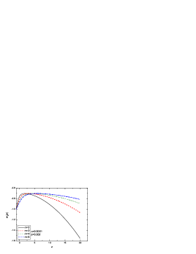
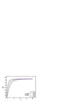
Figure 3: The interacting model of new agegraphic dark energy in Brans-Dicke theory. In this example, we fix $\alpha$ and $\beta$, and vary $n$.

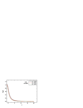
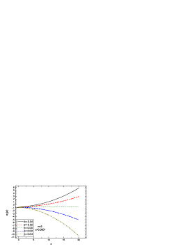
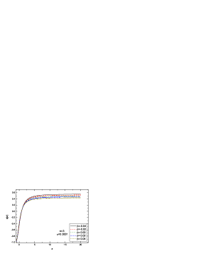
Figure 4: The interacting model of new agegraphic dark energy in Brans-Dicke theory. In this example, we fix $\alpha$ and $n$, and vary $\beta$.

To illustrate the cosmological evolution of the interacting model of new agegraphic dark energy in Brans-Dicke theory, we plot the fractional dark energy density $\Omega_{q}(z)$, the equation of state of dark energy $w_{q}(z)$ and the deceleration parameter $q(z)$ in Figs. 3 and 4. For the interacting case, the same initial condition $\Omega_{q}(z_{ini})=\frac{n^{2}(1+\alpha)^{2}}{4(1+z_{ini})^{2}}$ at $z_{ini}=2000$ can still be used, for the detailed discussion see Ref. [25]. First, to see the effect of the agegraphic model parameter $n$, as an example, we fix $\alpha=0.0001$ and $\beta=0.002$, and vary $n$ (from 2 to 5), as shown in Fig. 3. From this figure, it is very interesting to find that the interaction could break the early-time degeneracy in $w_{q}$ for various values of $n$ (see Fig. 2 for comparison). Next, to see the effect of the interaction parameter $\beta$, as an example, we fix $n=3$ and $\alpha=0.0001$, and vary $\beta$ (the value is taken as $-0.04$, $-0.02$, 0, $0.02$, and $0.04$, respectively), as shown in Fig. 4. From this figure, one can clearly see the impact of the interaction between dark energy and matter on the cosmological evolution of the new agegraphic dark energy model. It can be explicitly seen from the left panel of Fig. 4 that $\beta<0$ will lead to unphysical consequences in physics, since $\rho_{m}$ will become negative and $\Omega_{q}$ will be greater than 1 in the future. So, $\beta=b^{2}$ is commonly assumed in the literature.

6 Conclusion

In this note, we study the agegraphic dark energy model in the framework of Brans-Dicke gravitational theory. The Brans-Dicke theory is a natural alternative and a simple generalization of the Einstein’s general relativity. It is also the simplest example of a scalar-tensor gravitational theory. In the Brans-Dicke theory, the gravitational constant is replaced with the inverse of a time-dependent scalar field. We investigated how the agegraphic dark energy evolves in the universe in such a gravitational theory. In the Brans-Dicke cosmology, we derived the equation of state of dark energy $w_{q}(z)$ and the deceleration parameter $q(z)$ in both old and new versions of agegraphic dark energy model (in spit of the internal inconsistencies in the old version). In the usual cosmology, the agegraphic dark energy behaves like a quintessence: the old agegraphic dark energy looks like a thawing quintessence and the new agegraphic dark energy mimics a freezing quintessence. However, it is very interesting to find that in the Brans-Dicke theory of gravity the agegraphic dark energy (both old and new) realizes a quintom behavior, i.e., its equation of state crosses the phantom divide $w=-1$ during the evolution. We compared the situation of the agegraphic dark energy model in the Brans-Dicke theory with that in the Einstein’s theory. In addition, we also discussed the interaction model of the new agegraphic dark energy model in the Brans-Dicke theory.

References

- [1] A.G. Riess et al., Astron.J. 116, 1009 (1998); S. Perlmutter et al., ApJ 517, 565 (1999); J. L. Tonry et al., ApJ 594, 1 (2003); R.A. Knop et al., ApJ 598, 102 (2003); A.G. Riess et al., ApJ 607, 665 (2004).
- [2] S. Weinberg, Rev. Mod. Phys. 61, 1 (1989); arXiv:astro-ph/0005265; V. Sahni and A.A. Starobinsky, Int. J. Mod. Phys. D 9, 373 (2000); S.M. Carroll, Living Rev.Rel. 4, 1 (2001); P.J.E. Peebles and B. Ratra, Rev. Mod. Phys. 75, 559 (2003); T. Padmanabhan, Phys. Rept. 380, 235 (2003); E. J. Copeland, M. Sami and S. Tsujikawa, Int. J. Mod. Phys. D 15, 1753 (2006).
- [3] B. Ratra and P.J.E. Peebles, Phys. Rev. D37, 3406 (1988); P.J.E. Peebles and B.Ratra, ApJ 325, L17 (1988); C. Wetterich, Nucl. Phys. B302, 668 (1988); A&A 301, 321 (1995); I. Zlatev, L. Wang and P.J. Steinhardt Phys. Rev. Lett. 82, 896 (1999).
- [4] R.R. Caldwell, Phys. Lett. B 545, 23 (2002); S.M. Carroll, M. Hoffman and M. Trodden, Phys. Rev. D68, 023509 (2003).
- [5] B. Feng, X. L. Wang and X. M. Zhang, Phys. Lett. B 607 (2005) 35; Z. K. Guo, Y. S. Piao, X. M. Zhang and Y. Z. Zhang, Phys. Lett. B 608 (2005) 177; X. Zhang, Commun. Theor. Phys. 44 (2005) 762.
- [6] C. Armendariz-Picon, T. Damour and V. Mukhanov, Phys. Lett. B 458, 209 (1999); C. Armendariz-Picon, V. Mukhanov and P.J. Steinhardt, Phys. Rev. D63, 103510 (2001); T. Chiba, T. Okabe and M. Yamaguchi, Phys. Rev. D62, 023511 (2000).
- [7] H. Wei, R. G. Cai and D. F. Zeng, Class. Quant. Grav. 22, 3189 (2005); H. Wei and R. G. Cai, Phys. Rev. D 72, 123507 (2005).
- [8] T. Padmanabhan, Phys. Rev. D66, 021301 (2002); J.S. Bagla, H.K. Jassal, and T. Padmanabhan, Phys. Rev. D67, 063504 (2003).
- [9] A.Y. Kamenshchik, U. Moschella and V. Pasquier, Phys. Lett. B 511 265 (2001); M.C. Bento, O. Bertolami and A.A. Sen, Phys. Rev. D 66 043507 (2002); X. Zhang, F.Q. Wu and J. Zhang, JCAP 0601 003 (2006).
- [10] Y. Zhang, T.Y. Xia, and W. Zhao, Class. Quant. Grav. 24, 3309 (2007); T.Y. Xia and Y. Zhang, Phys. Lett. B 656, 19 (2007); S. Wang, Y. Zhang and T.Y. Xia, JCAP 10 037 (2008).
- [11] E. Witten, arXiv:hep-ph/0002297.
- [12] G. ’t Hooft, arXiv:gr-qc/9310026; L. Susskind, J. Math. Phys. 36, 6377 (1995).
- [13] M. Li, Phys. Lett. B 603, 1 (2004).
- [14] Q. G. Huang and M. Li, JCAP 0408, 013 (2004); JCAP 0503, 001 (2005); X. Zhang, Int. J. Mod. Phys. D 14, 1597 (2005); Phys. Rev. D 74, 103505 (2006); Phys. Lett. B 648, 1 (2007); M. R. Setare, J. Zhang and X. Zhang, JCAP 0703, 007 (2007); J. Zhang, X. Zhang and H. Liu, Eur. Phys. J. C 52, 693 (2007); Phys. Lett. B 651, 84 (2007); B. Wang, E. Abdalla and R. K. Su, Phys. Lett. B 611, 21 (2005); H. Wei and S. N. Zhang, Phys. Rev. D 76, 063003 (2007); X. Wu, R. G. Cai and Z. H. Zhu, Phys. Rev. D 77, 043502 (2008); B. Chen, M. Li and Y. Wang, Nucl. Phys. B 774, 256 (2007); M. Li, C. Lin and Y. Wang, JCAP 0805, 023 (2008); M. Li, X. D. Li, C. Lin and Y. Wang, Commun. Theor. Phys. 51, 181 (2009); S. Nojiri and S. D. Odintsov, Gen. Rel. Grav. 38, 1285 (2006).
- [15] B. Wang, Y. G. Gong and E. Abdalla, Phys. Lett. B 624, 141 (2005); B. Wang, C. Y. Lin and E. Abdalla, Phys. Lett. B 637, 357 (2006); B. Wang, C. Y. Lin, D. Pavon and E. Abdalla, Phys. Lett. B 662, 1 (2008); J. Zhang, X. Zhang and H. Liu, Phys. Lett. B 659, 26 (2008); B. Hu and Y. Ling, Phys. Rev. D 73, 123510 (2006); M. R. Setare, JCAP 0701, 023 (2007); E. N. Saridakis, Phys. Lett. B 661, 335 (2008); K. Karwan, JCAP 0805, 011 (2008); Y. Ma, Y. Gong and X. Chen, arXiv:0901.1215 [astro-ph]; E. Elizalde, S. Nojiri, S. D. Odintsov and P. Wang, Phys. Rev. D 71, 103504 (2005); L. Xu, arXiv:0907.1709 [astro-ph.CO]; Y. Gong and T. Li, arXiv:0907.0860 [hep-th].
- [16] X. Zhang and F. Q. Wu, Phys. Rev. D 72, 043524 (2005); Phys. Rev. D 76, 023502 (2007); Z. Chang, F. Q. Wu and X. Zhang, Phys. Lett. B 633, 14 (2006); M. Li, X. D. Li, S. Wang and X. Zhang, JCAP 0906, 036 (2009); Q. G. Huang and Y. G. Gong, JCAP 0408, 006 (2004); J. Y. Shen, B. Wang, E. Abdalla and R. K. Su, Phys. Lett. B 609, 200 (2005); Z. L. Yi and T. J. Zhang, Mod. Phys. Lett. A 22, 41 (2007); Y. Z. Ma, Y. Gong and X. Chen, Eur. Phys. J. C 60, 303 (2009); Q. Wu, Y. Gong, A. Wang and J. S. Alcaniz, Phys. Lett. B 659, 34 (2008).
- [17] R. G. Cai, Phys. Lett. B 657, 228 (2007).
- [18] F. Károlyházy, Nuovo Cim. A 42, 390 (1966); F. Károlyházy, A. Frenkel and B. Lukács, in Physics as Natural Philosophy, edited by A. Simony and H. Feschbach, MIT Press, Cambridge, MA (1982); F. Károlyházy, A. Frenkel and B. Lukács, in Quantum Concepts in Space and Time, edited by R. Penrose and C. J. Isham, Clarendon Press, Oxford (1986).
- [19] M. Maziashvili, Int. J. Mod. Phys. D 16, 1531 (2007).
- [20] M. Maziashvili, Phys. Lett. B 652, 165 (2007).
- [21] I. P. Neupane, Phys. Lett. B 673, 111 (2009).
- [22] H. Wei and R. G. Cai, Phys. Lett. B 660, 113 (2008).
- [23] J. Zhang, X. Zhang and H. Liu, Eur. Phys. J. C 54, 303 (2008).
- [24] H. Wei and R. G. Cai, Phys. Lett. B 663, 1 (2008); I. P. Neupane, Phys. Rev. D 76, 123006 (2007); Y. W. Kim, H. W. Lee, Y. S. Myung and M. I. Park, Mod. Phys. Lett. A 23, 3049 (2008); J. P. Wu, D. Z. Ma and Y. Ling, Phys. Lett. B 663, 152 (2008); J. Cui, L. Zhang, J. Zhang and X. Zhang, arXiv:0902.0716 [astro-ph.CO] (Chin. Phys. B, to be published).
- [25] L. Zhang, J. Cui, J. Zhang and X. Zhang, “Interacting model of new agegraphic dark energy: Cosmological evolution and statefinder diagnostic,” Int. J. Mod. Phys. D (submitted).
- [26] C. Brans and R. H. Dicke, Phys. Rev. 124 (1961) 925; R. H. Dicke, Phys. Rev. 125 (1962) 2163.
- [27] P. G. Bergmann, Int. J. Theor. Phys. 1 (1968) 25; J. Nordtvedt, Kenneth, Astrophys. J. 161 (1970) 1059; R. V. Wagoner, Phys. Rev. D 1 (1970) 3209; J. D. Bekenstein, Phys. Rev. D 15 (1977) 1458; J. D. Bekenstein and A. Meisels, Phys. Rev. D 18 (1978) 4378.
- [28] B. Bertotti, L. Iess and P. Tortora, Nature 425, 374 (2003).
- [29] C. Mathiazhagan and V.B. Johri, Class. Quantum Gravity 1, L29 (1984); D. La and P.J. Steinhardt, Phys. Rev. Lett. 62, 376 (1989); S. Das and N. Banerjee, arXiv:0803.3936.
- [30] F. Wu, L. e. Qiang, X. Wang and X. Chen, arXiv:0903.0384 [astro-ph.CO].
- [31] F. Wu and X. Chen, arXiv:0903.0385 [astro-ph.CO].
- [32] Y. Gong, Phys. Rev. D 70, 064029 (2004); M.R. Setare, Phys. Lett. B 644, 99 (2007); N. Banerjee, D. Pavon, Phys. Lett. B 647, 447 (2007); L. Xu and J. Lu, Eur. Phys. J. C 60, 135 (2009).
- [33] C. J. Feng, arXiv:0806.0673 [hep-th].
- [34] V. Acquaviva and L. Verde, JCAP 0712, 001 (2007).
- [35] L. Xu, J. Lu and W. Li, arXiv:0905.4174 [astro-ph.CO].
- [36] A. Sheykhi, arXiv:0908.0606 [gr-qc].