Pulsations in the late-type Be star HD 50 209 detected by CoRoT ^,

Abstract

Context. The presence of pulsations in late-type Be stars is still a matter of controversy. It constitutes an important issue to establish the relationship between non-radial pulsations and the mass-loss mechanism in Be stars.

Aims. To contribute to this discussion, we analyse the photometric time series of the B8IVe star HD 50 209 observed by the CoRoT mission in the seismology field.

Methods. We use standard Fourier techniques and linear and non-linear least squares fitting methods to analyse the CoRoT light curve. In addition, we applied detailed modelling of high-resolution spectra to obtain the fundamental physical parameters of the star.

Results. We have found four frequencies which correspond to gravity modes with azimuthal order $m=0,-1,-2,-3$ with the same pulsational frequency in the co-rotating frame. We also found a rotational period with a frequency of $0.679$ $\mbox{cd}^{-1}$(7.754 $\mu$Hz).

Conclusions. HD 50 209 is a pulsating Be star as expected from its position in the HR diagram, close to the SPB instability strip.

1 Introduction

Classical Be stars are defined as main sequence or slightly evolved B-type stars whose spectrum has or had at some time one or more Balmer lines in emission. They are physically understood as rapidly rotating B-type stars with line emission arising from a circumstellar disk in the equatorial plane, composed of matter ejected from the stellar photosphere by mechanisms not yet understood (see Porter & Rivinius 2003, for a complete review). A significant fraction of Be stars show short-term photometric and spectroscopic periodic variability, which is commonly attributed to non-radial pulsations. As Be stars occupy the same region of the HR diagram as $\beta$ Cephei and SPB stars, it is generally assumed that pulsations have the same origin, i.e. p- and/or g-mode pulsations driven by the $\kappa$-mechanism associated with the Fe bump. The current theoretical models have difficulties in describing the pulsational characteristics of Be stars, due to the high rotational velocity of these objects. A brief description of the current knowledge of the pulsational behavior of Be stars can be found in Neiner et al. (2009) and Emilio et al. (2009).

HD 50 209 is a late Be star of spectral type B8IVe and magnitude $V=8.36$. It has been studied by Gutiérrez-Soto et al. (2007), using data from Hipparcos, ASAS-3 and the OSN (Observatorio de Sierra Nevada). The Hipparcos data analysis yielded a frequency of variation at 1.689 $\mbox{cd}^{-1}$considered as uncertain and another frequency at 1.47 $\mbox{cd}^{-1}$, although with a lower amplitude. From OSN, the analysis revealed a frequency at 1.4889 $\mbox{cd}^{-1}$. The analysis of the ASAS-3 dataset showed significant peaks at frequency 2.4803 $\mbox{cd}^{-1}$and 1.4747 $\mbox{cd}^{-1}$.

The occurrence of pulsations in late B-type stars has been a matter of controversy in the recent literature. Hubert & Floquet (1998) showed that pulsations in B6-B9 type stars are much less common than in their early-type counterparts. Baade (1989) failed to detect line profile variations in the spectra of B8-B9.5 stars. However, Saio et al. (2007) presented the detection of low amplitude g-modes in the B8Ve star $\beta$ CMi. To ascertain whether Be stars of all types do present pulsations is a key issue in order to establish the relation between non-radial pulsations and the mass ejection mechanisms.

The CoRoT satellite (Auvergne et al. 2009) observed HD 50 209 in its seismology field. The observations span 136 days in the Galactic anti-centre direction (LRA1), between October 18th 2007 and March 3rd 2008, with a sampling of 32 seconds. The light curve contains 328 279 data-points with a duty cycle of $89\%$.

2 Frequency analysis

For the frequency analysis, we employed the code pasper (Diago et al. 2008), which is based on the classical discrete Fourier transform (Deeming 1975; Scargle 1982) and the least-square fitting of a sinusoidal function in the time domain. When a frequency is found, it is prewhitened from the original data and a new step starts looking for a new frequency in the residuals. The method is iterative and stops when the new frequency is not statistically significant.

The criterion used to determine whether the frequencies are statistically significant is the signal to noise amplitude ratio requirement described in Breger et al. (1993). It consists of the calculation of the SNR of the frequency in the periodogram. This is made calculating the signal as the amplitude of the peak for the frequency obtained and the noise as the average amplitude in the residual periodogram after the prewhitening of all the frequencies detected. Breger et al. (1993) proposed that a value of SNR $\geq 4$ is a reliable criterion to distinguish between peaks due to real frequencies and noise.

All the techniques used in this paper are described in detail by Gutiérrez-Soto et al. (2009). As mentioned in that paper, the orbital characteristics of the CoRoT satellite produces signal in the data at the orbital frequency ($13.97$ $\mbox{cd}^{-1}$, 161.689 $\mu$Hz) and day/night peaks ($2.007$ $\mbox{cd}^{-1}$, 23.229 $\mu$Hz) and their harmonics. All those frequencies of instrumental origin have been removed from the list of detected frequencies.

The resolution in frequency of our analysis is $1/2\,T\sim 3.66\times 10^{-3}$ $\mbox{cd}^{-1}$(Kallinger et al. 2008), $T$ being the total interval covered by observations. The uncertainty on the detected frequencies is $\sqrt{3}\times 10^{-6}$ $\mbox{cd}^{-1}$. This value has been derived analytically using the formula given by Montgomery & O’Donoghue (1999), and taking into account the correlations in the residuals, as described by Schwarzenberg-Czerny (1991).

Table 1: Principal frequencies of each set detected in HD 50 209.

Set	Freq.	Freq.	Amp.	Main freq.	Comment.
	[$\mbox{cd}^{-1}$]	[$\mu$Hz]	[mmag]
$F_{1}$	1.48444	17.181	2.529	$f_{1}$	$f_{5}+2\,f_{4}$
	1.49028	17.248	1.616
	1.47860	17.113	1.090
	1.49613	17.316	0.653
$F_{2}$	2.16238	25.027	0.904	$f_{2}$	$f_{5}+3\,f_{4}$
	2.16822	25.095	0.495
$F_{3}$	0.79482	9.199	0.607	$f_{3}$	$f_{5}+f_{4}$
	0.77874	9.013	0.407
	0.80650	9.334	0.358
$F_{4}$	0.67939	7.863	0.425	$f_{4}$	$f_{rot}$
	0.69108	7.998	0.368
$F_{5}$	0.10811	1.251	0.202	$f_{5}$
$F_{6}$	2.96889	34.362	0.121	$f_{6}$	$2\,f_{1}$

Figure 1: Top: CoRoT light curve of the star HD 50 209. Bottom: CoRoT light curve detrended with a polynomial of second degree.

Figure 2: Left: Complete Fourier spectrum for HD 50 209 showing aliasing effects at the orbital frequency 13.97 $\mbox{cd}^{-1}$. Right: Fourier spectrum for HD 50 209 in the domain of the detected stellar frequencies.

Figure 3: The 60 significant frequencies detected for the star HD 50 209 revealing six different and separated frequency groups.

In Fig. 1 (top panel) we present the CoRoT light curve of HD 50 209. A long-term decreasing pattern is apparent. It is a common feature of the CoRoT light curves to show a linear or an almost linear decreasing pattern of instrumental origin due to the CCD ageing. On the other hand, most Be stars present long-term variations which in our case contribute to the observed variability. We have removed these trends by fitting a polynomial function of second degree without making assumptions on their origin, obtaining the light curve depicted in the bottom panel of Fig. 1.

Table 2: Complete list of significant frequencies obtained with pasper for the star HD 50 209. The time reference for the phase is HJD = 2454391.95. The full table is available online.

#	Freq.	Freq.	Amp.	Amp. error	Phase	Phase error	S/N	Comment.
	[$\mbox{cd}^{-1}$]	[$\mu$Hz]	[mmag]	[mmag]	[0,1]	[0,1]
1	1.48444	17.181	2.5299	0.0011	0.7348	0.0001	265	$f_{1}$
2	1.49028	17.2486	1.6167	0.0012	0.1577	0.0001	169
3	1.47860	17.1134	1.0901	0.0011	0.2747	0.0002	114
4	2.16238	25.0275	0.9043	0.0010	0.9746	0.0002	94	$f_{2}$
5	0.79482	9.19931	0.6077	0.0011	0.9866	0.0003	63	$f_{3}$
$\cdots$	$\cdots$	$\cdots$	$\cdots$	$\cdots$	$\cdots$	$\cdots$	$\cdots$	$\cdots$

In Fig. 2 we display the Fourier spectrum, showing the typical aliasing at the orbital frequency (as described in Gutiérrez-Soto et al. 2009). From the frequency analysis, we obtain 60 significant frequencies which are listed in Table 2 (full table only available online). Note that frequencies around $3/T\sim 0.022$ $\mbox{cd}^{-1}$(0.255 $\mu$Hz) or lower correspond to periods of the order of the entire dataset time-span, and hence should be considered with caution. They might be produced by the detrending process or artifacts of the frequency analysis. However, we have included them for completeness.

The entire set of detected frequencies together with their amplitudes is plotted in Fig. 3. The frequencies found are distributed in 6 main groups ($F_{i}$ with $i=1,...,6$). The frequencies with the highest amplitudes are listed in Table 1. All groups are clearly separated, except those centered on $f_{3}$ and $f_{4}$. In each group we note the existence of equidistant multiplets separated by intervals marginally larger than our frequency resolution. In Fig. 4 we provide the diagrams of the folded light curve with the two main frequencies $f_{1}$ and $f_{2}$.

Figure 4: Top: Phase diagram for the HD 50 209 data folded with the frequency $f_{1}=1.48444$ $\mbox{cd}^{-1}$(17.181 $\mu$Hz). Bottom: Phase diagram for the HD 50 209 data, prewhitened from the frequency $f_{1}$ and folded with the frequency $f_{2}=2.16238$ $\mbox{cd}^{-1}$(25.027 $\mu$Hz). Note that two cycles are shown for clarity.

In addition, we performed a time-frequency analysis of the original light curve by applying the pasper code to sliding windows with different sizes (for details on the method, see Huat et al. 2009). The results presented in Fig. 5 show that all the main frequencies show large amplitude changes. See Section 4 for a detailed discussion of these changes.

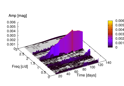
Figure 5: 3-D view of the frequencies determined using the time-frequency analysis with a sliding window of 30 days. The color scale indicates the amplitude of the detected frequencies in HD 50 209. The time origin corresponds to HJD = 2454391.95.

3 Ground-based observations

High resolution spectroscopy of HD 50 209 was obtained with the FEROS spectrograph at the 2.2m telescope in La Silla, in the framework of a large program complementary to the CoRoT mission. Observations were carried out one year prior to the LRA1 run of CoRoT to investigate spectroscopically the rapid variability previously detected in photometry by Gutiérrez-Soto et al. (2007). Seventy spectra with high spectral resolution and high signal-to-noise ratio were obtained. Fourteen additional spectra were obtained with the Narval spectropolarimeter at the TBL at Pic du Midi Observatory (France), contemporary to the CoRoT run. However, due to bad weather conditions, the signal-to-noise ratio is not high enough to search for low amplitude variability in the Narval data.

FEROS observations ($R=48000$, $3600-9200$ Å) were reduced with MIDAS (wavelength calibration, bias and flat field corrections and earth motion correction). For the Narval observations ($R=65000$) the sum of the 4 sub-exposures obtained in Stokes V sequences were used. Exposures were reduced locally with LibrEsprit based on the Esprit software (Donati et al. 1997) and then summed. The continuum normalization was carried out with IRAF.

The fundamental physical parameters of HD 50 209 have been accurately determined from the newly available spectroscopic data adopting a procedure described by Frémat et al. (2006) and correcting for gravitational darkening effects (Frémat et al. 2005). The obtained parameters are derived by fitting to the spectra, adopting the different values of $\Omega/\Omega_{c}$ presented in the first row of Table 3. The results are presented in Table 3 and are consistent with the previous parameter determination (Frémat et al. 2006).

Table 3: Fundamental parameters for HD 50 209 computed for different values of $\Omega/\Omega_{c}$ and corrected for veiling. The errors in $T_{eff}$, $\log g$ and $V\,\sin\,i$ are taken from the apparent parameters.

$\Omega/\Omega_{c}$	$i$	$T_{\rm eff}$	$\log g$	$V\,\sin\,i$	$M$	$L$	$R_{\rm eq}$	$f_{\rm rot}$
	[deg]	[K]	[cgs]	[km/s]	[$M_{\odot}$]	[$L_{\odot}$]	[$R_{\odot}$]	[$\mbox{cd}^{-1}$]
0.80	$89\pm 20$	$13600\pm 1500$	$3.60\pm 0.11$	$192\pm 20$	$4.67\pm 0.95$	$2.97\pm 0.39$	$6.44\pm 1.53$	$0.60\pm 0.20$
0.90	$64\pm 14$	$13600\pm 1500$	$3.56\pm 0.11$	$205\pm 20$	$4.76\pm 1.02$	$3.02\pm 0.39$	$7.27\pm 1.74$	$0.62\pm 0.20$
0.95	$57\pm 15$	$13600\pm 1500$	$3.53\pm 0.11$	$211\pm 20$	$5.07\pm 1.15$	$3.08\pm 0.40$	$8.06\pm 2.03$	$0.62\pm 0.22$
0.99	$55\pm 12$	$13400\pm 1500$	$3.46\pm 0.11$	$221\pm 20$	$4.99\pm 1.22$	$3.14\pm 0.41$	$9.34\pm 2.35$	$0.58\pm 0.20$

Spectroscopic data also show that emission is present in the first Balmer lines and visible up to H$\delta$. H$\alpha$ is a strong emission line ($EW=-19$ Å , $Imax=4.68$ Icont) with inflection points on the wings and close double peaks at the centre. The line profile is typical of a Be star seen under a moderate inclination angle (Hanuschik et al. 1996). H$\beta$, H$\gamma$ and H$\delta$ show a symmetrical and double-peaked emission embedded in the broad wings of the photospheric profile. Moreover, numerous Fe ii and Cr ii lines as well as the IR Ca ii triplet and O i 8446 $\AA$ lines are in emission with a double component. Note that we have not found significant changes in the global emission state of HD 50 209 between the FEROS and Narval spectra taken about one year apart.

In addition, forbidden single-peaked [O i] 6300 $\AA$ and [Fe ii] emission lines are detected with a very weak intensity ($I\leq 1.01\%$ of the continuum, see Fig. 6). The star is isolated, outside any formation region, and without the large IR excess typical of HAeBe stars. It could be an extreme Be star according to de Winter & Pérez (1998) or an unclB[e] star in the scheme proposed by Lamers et al. (1998), though the B[e] character is very weak.

Figure 6: Top: Forbidden emission line of [O i] at 6300 $\AA$. Bottom: Three forbidden emission lines of [Fe ii] at 4244.1 $\AA$ (21F), 4276.9 $\AA$ (21F) and 4287.5 $\AA$ (7F) from the spectra of HD 50 209.

Figure 7: Left panels: H$\alpha$ and H$\beta$ emission. Right panels: Different emission lines in the Fe ii region in the star HD 50 209. In all panels the horizontal axis is wavelength and the vertical one is relative intensity.

The mean H$\alpha$, H$\beta$ and Fe II 5197.6 $\AA$ and 5316.6 $\AA$ profiles are shown in Fig. 7. The separation between the emission peaks and the lack of a shell profile exclude an inclination angle close to 90 degrees, and hence the physical parameters in the first row of Table 3 are not suitable. This implies that the rotational frequency is at least 90% of the critical velocity. The shape of the H$\alpha$ line profile and the forbidden lines discussed above indicate the presence of a very extended circumstellar disk.

In spite of the high quality of the FEROS spectra and the presence of rapid photometric variability apparent in the CoRoT data (see Fig. 1), we have not been able to detect periodic variability in purely photospheric lines of HD 50 209. Some variability is present slightly above the detection limit but no consistent periodic behavior could be established. Weak rapid variations were detected in the intensity of the $V$ and $R$ emission components of Balmer lines and their $V/R$ ratio. Note also that the quantity $(V+R)/2$ seems to be slightly lower in the second part of the ESO run, suggesting a slight weakening of the emissivity of the disk. As shown in the mean variance in the H$\beta$ profile, the variability is concentrated in the emission part. Note that the variability is more conspicuous on certain days. Unfortunately, the gap between the two parts of the ESO run, the alternating of day/night and the weakness of variations prevent any reliable estimate on the time-scale of variations.

4 Discussion

As a result of our analysis, we have obtained 60 significant frequencies, grouped in six sets. In each set, different equidistant frequencies close to the main detected ones are present. The Fourier analysis of the light curve by means of sliding windows results in the detection of a significant variation of amplitude of the main frequencies (Fig. 5).

The first issue to be addressed is the presence of frequency multiplets and amplitude variations. Both phenomena are related, and can be due either to the presence of close frequencies or actual amplitude variations (Breger & Pamyatnykh 2006). The beating of two or more close frequencies will appear as a single frequency with variable amplitude when we split the data sample in shorter intervals, with the consequent loss of frequency resolution. On the other hand, true amplitude variability will produce peaks in the power spectrum broader than expected from the frequency resolution (Fig. 8), and the prewhitening of the main frequency will leave power in the wings of the main peak which will lead to false frequency doublets or multiplets.

Figure 8: Periodogram of the original light curve (solid line) and spectral window shifted at $f_{1}=1.48444$ $\mbox{cd}^{-1}$(dashed line). Note that the full width at half maximum of the peak in the periodogram at the frequency $f_{1}$ is broader than expected from the spectral window, suggesting the presence of more frequencies or amplitude changes. The vertical line indicates the position of the frequency $f_{1}$.

In order to discriminate between the beating of several frequencies and an amplitude change of a single frequency we have applied the method described in Breger & Pamyatnykh (2006) to study the relationship between amplitude variability and phase variations of an assumed single frequency. The idea behind this method is that the beating of frequencies will produce a phase variation with the same period as the beating period, while in the case of a single frequency with variable amplitude, the phase will remain constant.

We studied the six frequency groups with the abovementioned method. However, the results obtained are inconclusive, for two main reasons: i) the beat periods of the close frequencies are larger than the time coverage of CoRoT data, and hence, we cannot evaluate the consistency of the phase variations; ii) the phase variations predicted by the models with four or more frequencies are very small. At our detection level we were not able to discriminate between the predicted low amplitude variations and no variation at all. Consequently, we cannot firmly reject either of the two interpretations.

In the following, we analyze the six main frequencies found, which, as discussed above, can be either single frequencies with variable amplitude or groups of close frequencies around a central value. The highest frequency, $f_{6}$, is the first harmonic of $f_{1}$, i.e. $f_{6}=2\,f_{1}$, and hence it will not be considered in the analysis. Frequencies $f_{5}$, $f_{3}$, $f_{1}$ and $f_{2}$ are equidistant within the frequency resolution at the 3-$\sigma$ level, and the separation between them is the frequency $f_{4}$. Moreover, $f_{4}=0.67939$ $\mbox{cd}^{-1}$is consistent with the rotational frequency of the star as given in Table 3. As a consequence, we have only two independent main frequencies, $f_{4}$ and $f_{5}$, and all the others are of the form $f_{i}=f_{5}+n\,f_{4}$ with $n=1,2,3$.

Let us recall that the observed frequencies in a rotating star are related to the pulsational frequency in the co-rotating frame by the expression:

$$\nu=\,|\,\overline{\nu}-m\,\Omega\,|$$ (1)

where $\overline{\nu}$ is the frequency in the co-rotating frame and $\Omega$ is the rotational frequency of the star. From this expression, and considering $f_{4}$ as the rotational frequency as discussed above, the four frequencies $f_{5}$, $f_{3}$, $f_{1}$ and $f_{2}$ can be consistently interpreted as modes with the same pulsational frequency in the co-rotating frame and with $m=0,-1,-2,-3$ respectively.

The fundamental parameters presented in Table 3 place HD 50 209 marginally outside the SPB instability strip calculated by Pamyatnykh (1999), although its position is compatible with the strip at the 1-$\sigma$ error level. Hence, we consider that the pulsations detected are gravity modes typical of SPB stars. HD 50 209 is a SPBe star, the designation proposed by Walker et al. (2005) for the Be stars pulsating in g-modes, considered as rapidly rotating counterparts of the SPB stars.

Due to the fact that in late-type B stars the frequencies of the g-modes in the co-rotating frame are much smaller than the rotational frequency, the frequencies of these modes in the observer’s frame are close to $|\,m\,\Omega\,|$. This leads to the difficulty that the observed frequencies close to the expected rotational frequency can be either interpreted as g-mode pulsations (Walker et al. 2005) or as rotational modulation (Balona 1995). In our case, we can for the first time discriminate between the rotational frequency and the frequency of the g-mode pulsation with azimuthal order $|\,m\,|=1$, as we have detected both of them clearly separated by an interval much larger than the frequency resolution, thanks to the long duration of observations and precise measurements of CoRoT. We can be confident that the frequencies $f_{5}$, $f_{3}$, $f_{1}$ and $f_{2}$ are not related to the rotation and hence they are true gravity mode pulsations.

The frequency in the co-rotating frame of the detected modes, namely $f_{5}=0.10811$ $\mbox{cd}^{-1}$, is significantly lower than the frequencies commonly found for both SPB and SPBe stars. However, this low value is consistent with what is expected for an $m=0$ mode in models of rapidly rotating late-type B stars (Walker et al. 2005; Saio et al. 2007). The modelling of the detected pulsations will provide more insights into the nature of the pulsational modes.

5 Conclusions

The high precision photometry and long duration of continuous observations provided by the CoRoT mission has allowed the detection of g-mode pulsations in the late-type Be star HD 50 209. This supports the fact that all Be stars have non-radial pulsations that could play a critical role in the mass ejection mechanism.

From our analysis, we have found pulsation in four modes with the same frequency in the co-rotating frame with azimuthal order $m=0,-1,-2,-3$. We have also detected the rotational frequency, both as a significant peak in the power spectrum and as the separation of frequencies with different $m$. The accurate determination of the rotational period will play an important part in constraining the fundamental parameters of the star in order to perform the seismic modelling.

For the first time, we have been able to observe simultaneously the rotational frequency and the pulsational frequencies and separate them, implying that the frequencies we attribute to g-mode pulsations cannot be interpreted as the effect of the rotational modulation. This constitutes a proof of the presence of pulsations in HD 50 209.

2

Table 4: Complete list of significant frequencies obtained with pasper for the star HD 50 209. The time reference for the phase is HJD = 2454391.95.

#	Freq.	Freq.	Amp.	Amp. error	Phase	Phase error	S/N	Comment.
	[$\mbox{cd}^{-1}$]	[$\mu$Hz]	[mmag]	[mmag]	[0,1]	[0,1]
1	1.48444	17.181	2.5299	0.0011	0.7348	0.0001	265	$f_{1}$
2	1.49028	17.2486	1.6167	0.0012	0.1577	0.0001	169
3	1.47860	17.1134	1.0901	0.0011	0.2747	0.0002	114
4	2.16238	25.0275	0.9043	0.0010	0.9746	0.0002	94	$f_{2}$
5	0.79482	9.19931	0.6077	0.0011	0.9866	0.0003	63	$f_{3}$
6	1.49613	17.3163	0.6531	0.0011	0.2873	0.0003	68
7	2.16822	25.0951	0.4953	0.0010	0.2636	0.0003	51
8	0.01461	0.16909	0.4324	0.0010	0.2149	0.0004	45	$<3/T$
9	0.77874	9.01319	0.4074	0.0010	0.0079	0.0004	42
10	0.80650	9.33449	0.3583	0.0010	0.4104	0.0005	37
11	0.67939	7.86331	0.4256	0.0010	0.3579	0.0004	44	$f_{4}$
12	0.69108	7.99861	0.3685	0.0009	0.5289	0.0004	38
13	0.82258	9.5206	0.2768	0.0010	0.4198	0.0006	29
14	0.80066	9.2669	0.2740	0.0011	0.1969	0.0006	28
15	0.10811	1.25127	0.2030	0.0010	0.5750	0.0008	21	$f_{5}$
16	0.81527	9.436	0.1725	0.0009	0.2895	0.0009	18
17	0.78897	9.1316	0.1214	0.0011	0.8024	0.0014	12
18	0.09350	1.08218	0.1509	0.0009	0.4966	0.0010	15
19	0.03506	0.40578	0.1359	0.0009	0.3221	0.0011	14
20	0.11396	1.31898	0.1647	0.0010	0.7770	0.0010	17
21	1.51074	17.4854	0.1217	0.0009	0.2095	0.0012	12
22	0.65894	7.62662	0.1333	0.0010	0.2271	0.0011	13
23	2.96889	34.3622	0.1210	0.0009	0.7144	0.0012	12	$f_{6}$
24	0.07451	0.86238	0.0862	0.0009	0.2504	0.0017	9
25	0.64725	7.49132	0.0980	0.0009	0.1021	0.0015	10
26	0.82842	9.58819	0.1421	0.0010	0.7036	0.0011	14
27	0.00876	0.10138	0.1040	0.0010	0.6659	0.0015	10	$<3/T$
28	0.11980	1.38657	0.1164	0.0010	0.9496	0.0013	12
29	0.83573	9.6728	0.1160	0.0010	0.5225	0.0013	12
30	1.50197	17.3839	0.1158	0.0011	0.4101	0.0014	12
31	0.84157	9.74039	0.1131	0.0010	0.7923	0.0014	11
32	0.66916	7.74491	0.0847	0.0009	0.0830	0.0018	8
33	0.74952	8.675	0.0751	0.0009	0.0087	0.0019	7
34	0.04967	0.57488	0.1041	0.0009	0.5844	0.0014	10
35	0.70131	8.11701	0.0854	0.0009	0.8694	0.0017	8
36	0.02337	0.27048	0.0867	0.0009	0.2750	0.0017	9	$\sim 3/T$
37	0.06136	0.71018	0.0894	0.0009	0.8152	0.0017	9
38	0.56397	6.52743	0.0792	0.0009	0.1145	0.0018	8
39	1.45668	16.8597	0.0774	0.0009	0.4253	0.0019	8
40	0.62533	7.23762	0.0694	0.0009	0.1556	0.0021	7
41	0.54205	6.27373	0.0726	0.0009	0.8328	0.0020	7
42	0.86203	9.9772	0.0731	0.0009	0.7081	0.0020	7
43	2.15361	24.926	0.0749	0.0009	0.2862	0.0019	7
44	0.72030	8.33681	0.0829	0.0009	0.8066	0.0018	8
45	2.96158	34.2775	0.0672	0.0009	0.4195	0.0021	7
46	0.73199	8.47211	0.0681	0.0009	0.0589	0.0022	7
47	0.12711	1.47118	0.0683	0.0009	0.1174	0.0021	7
48	2.97619	34.4466	0.0640	0.0009	0.0250	0.0022	6
49	2.17406	25.1627	0.0875	0.0010	0.5229	0.0019	9
50	2.17991	25.2304	0.0755	0.0010	0.7423	0.0021	7
51	1.53996	17.8236	0.0590	0.0009	0.4461	0.0024	6
52	0.77290	8.9456	0.0615	0.0010	0.8969	0.0025	6
53	1.38363	16.0142	0.0553	0.0009	0.7286	0.0026	5
54	0.47484	5.49583	0.0574	0.0009	0.4781	0.0025	6
55	0.61510	7.11921	0.0560	0.0009	0.2581	0.0026	5
56	1.52535	17.6545	0.0559	0.0009	0.2121	0.0026	5
57	0.87079	10.0786	0.0642	0.0009	0.8295	0.0023	6
58	0.88394	10.2308	0.0567	0.0009	0.9051	0.0026	5
59	0.58150	6.73032	0.0525	0.0009	0.6858	0.0028	5
60	0.17971	2.07998	0.0515	0.0009	0.1046	0.0028	5