Quantum Tunneling and Unitarity Features of an $\boldsymbol{S}$-matrix for Gravitational Collapse

Abstract

Starting from the semiclassical reduced-action approach to transplanckian scattering by Amati, Veneziano and one of us and from our previous quantum extension of that model, we investigate the $S$-matrix expression for inelastic processes by extending to this case the tunneling features previously found in the region of classical gravitational collapse. The resulting model exhibits some non-unitary $S$-matrix eigenvalues for impact parameters $b<b_{c}$, a critical value of the order of the gravitational radius $R=2G\sqrt{s}$, thus showing that some (inelastic) unitarity defect is generally present, and can be studied quantitatively. We find that $S$-matrix unitarity for $b<b_{c}$ is restored only if the rapidity phase-space parameter $y$ is allowed to take values larger than the effective coupling $Gs/\hbar$ itself. Some features of the resulting unitary model are discussed.

DFF 451/09/2009

1 Introduction

The ACV eikonal approach to string-gravity at planckian energies [1] has been recently investigated in the region of classical gravitational collapse. A simplified version of it — the reduced-action model of Amati, Veneziano and one of us [2] — has been extensively studied at semiclassical level [2, 3, 4], and has been extended by us (CC) to a quantum level [5]. The main feature of such a model is the existence of a critical impact parameter $b=b_{c}$ of the order of the gravitational radius $R\equiv 2G\sqrt{s}$, such that, for $b<b_{c}$, a classical gravitational collapse is expected to occur, while the elastic semiclassical $S$-matrix shows an exponential suppression driven by the effective coupling $\alpha\equiv Gs/\hbar$ [2]. This suppression admits in turn a tunneling interpretation at quantum level [5], corresponding to a partial information recovery, compared to classical information loss.

The purpose of the present paper is to further study the CC quantum model, in particular its extension to inelastic processes in order to see whether the tunneling suppression of the elastic channel is possibly compensated by inelastic production thus recovering $S$-matrix unitarity.

The point above is perhaps the key question that the ACV approach is supposed to clarify. Indeed, if our $S$-matrix model well represents the original string-gravity theory, then unitarity is expected irrespective of whether classical collapse may occur for $b<b_{c}$. This could be interpreted as full information recovery at quantum level (compared to classical information loss) because the suppression of the elastic channel is compensated by the inelastic ones.

Unfortunately, the situation is not a clearcut one, because of the approximations involved in the model. On one hand, the reduced-action approach neglects string and rescattering corrections which — as argued in [2] — could come in together because of the strong-coupling and, eventually, of the short distances involved. Furthermore the quantum-extension of [5] is admittedly incomplete because quantum fluctuations involve only the transverse-distance dependence of the metric fields, while keeping the classical shock-wave space-time dependence as frozen. Finally, our extension of the $S$-matrix to inelastic processes is based on a weak-coupling procedure which neglects correlations and possible bound states, assumptions which could fail in a strong-coupling configuration.

Indeed, we find eventually that the model shows a unitarity defect for $b<b_{c}$, which is dependent on the rapidity phase-space parameter $y$, in such a way that unitarity is recovered in the $y\to\infty$ limit only. This result is interesting because we do have a non-trivial unitary model at large $y$’s and all $b$’s. But it is puzzling also, because it leaves open the question of whether, for moderate $y$, one of the simplifying assumptions above went wrong, or whether instead a unitarity defect is a possible feature of quantum gravity in the classical collapse region.

In order to introduce the subject properly, we summarize in sec. 2 both the semiclassical ACV results for the $S$-matrix and the CC quantum extension, by emphasizing its tunneling interpretation in the elastic channel. In sec. 3 we derive an improved integral representation of the CC tunneling amplitude which is applicable for any values of the $y$-parameter, and we discuss the role of absorption for the various regimes of the elastic amplitude. We start discussing inelastic processes in sec. 4, where we provide two classes of $S$-matrix eigenstates, one corresponding to a weak-field coherent state which exhibits a unitarity defect for $b<b_{c}$, and the other with unitary eigenvalues at all $b$’s, which requires a suitably chosen strong-field configuration. The ensuing expectations on the unitarity defect around the elastic channel are compared to the direct path-integral evaluation of $S^{\dagger}S$ in sec. 5. We find the $y$-dependent unitarity defect mentioned previously, that we have quantitatively evaluated at semiclassical level. We also describe the main features of the unitary large-$y$ model, by discussing in sec. 6 possible hints of further improvements.

2 The reduced-action approach to gravitational $\boldsymbol{S}$-matrix

2.1 The semiclassical ACV results

The simplified ACV approach [2] to transplanckian scattering is based on two main points. Firstly, the gravitational field $g_{\mu\nu}=\eta_{\mu\nu}+h_{\mu\nu}$ associated to the high-energy scattering of light particles, reduces to a shock-wave configuration of the form

$$h_{--}\big{|}_{x^{+}=0} =(2\pi R)a(\boldsymbol{x})\delta(x^{-})\;,\qquad h_{++}\big{|}_{x^{-}=0}=(2\pi R)\bar{a}(\boldsymbol{x})\delta(x^{+})$$ (1a)

$$h_{ij} =(\pi R)^{2}\Theta(x^{+}x^{-})\left(\delta_{ij}-\frac{\partial_{i}\partial_{j}}{\nabla^{2}}\right)h(\boldsymbol{x})\;,$$ (1b)

where $a$, $\bar{a}$ are longitudinal profile functions, and $h(\boldsymbol{x})\equiv\nabla^{2}\phi$ is a scalar field describing one emitted-graviton polarization (the other, related to soft graviton radiation, is negligible in an axisymmetric configuration).

Secondly, the high-energy dynamics itself is summarized in the $h$-field emission-current $\mathcal{H}(\boldsymbol{x})$ generated by the external sources coupled to the longitudinal fields $a$ and $\bar{a}$. Such a vertex has been calculated long ago [6, 7] and takes the form

$$-\nabla^{2}\mathcal{H}\equiv\nabla^{2}a\nabla^{2}\bar{a}-\nabla_{i}\nabla_{j}a\nabla_{i}\nabla_{j}\bar{a}\;,$$ (2)

which is the basis for the gravitational effective action [8, 9, 10] from which the shock-wave solution (1) emerges [1]. It is directly coupled to the field $h$ and, indirectly, to the external sources $s$ and $\bar{s}$ in the reduced 2-dimensional action

$$\frac{{\cal A}}{2\pi Gs}=\int\mathrm{d}^{2}\boldsymbol{x}\left(a\bar{s}+\bar{a}s-\frac{1}{2}\nabla a\nabla\bar{a}+\frac{(\pi R)^{2}}{2}\left(-(\nabla^{2}\phi)^{2}-2\nabla\phi\cdot\nabla\mathcal{H}\right)\right)$$ (3)

which is the basic ingredient of the ACV simplified treatment.

The equations of motion (EOM) induced by (3) provide, with proper boundary conditions, some well-defined effective metric fields $a$ and $h$. The “on-shell” action ${\cal A}(b,s)$, evaluated on such fields, provides directly the elastic $S$-matrix

$$S_{\mathrm{el}}=\exp\left(\frac{\mathrm{i}}{\hbar}{\cal A}(b,s)\right).$$ (4)

Then, it can be shown [1, 2] that the reduced-action above (where $R$ plays the role of coupling constant) resums the so-called multi-H diagrams (fig. 1), contributing a series of corrections $\sim(R^{2}/b^{2})^{n}$ to the leading eikonal.

+         + …

Figure 1: Diagrammatic series of H and multi-H diagrams.

Furthermore, the $S$-matrix (4) can be extended to inelastic processes on the basis of the same emitted-graviton field $h(\boldsymbol{x})$. In the eikonal formulation the inelastic $S$-matrix is approximately described by the coherent state operator

$$S=\exp\left(\frac{\mathrm{i}}{\hbar}{\cal A}(b,s)\right)\exp\left(\mathrm{i}2\pi R\sqrt{\alpha}\int\mathrm{d}^{2}\boldsymbol{x}\;h(\boldsymbol{x})\Omega(\boldsymbol{x})\right)$$ (5)

$$\Omega(\boldsymbol{x})\equiv\int\frac{\mathrm{d}^{2}\boldsymbol{k}\,\mathrm{d}k_{3}}{2\pi\sqrt{k_{0}}}\left[a(\boldsymbol{k},k_{3})\mathrm{e}^{\mathrm{i}\boldsymbol{k}\cdot\boldsymbol{x}}+h.c.\right]\equiv A(\boldsymbol{x})+A^{\dagger}(\boldsymbol{x})\;,$$

$$[A(\boldsymbol{x}),A^{\dagger}(\boldsymbol{x}^{\prime})]=Y\delta(\boldsymbol{x}-\boldsymbol{x}^{\prime})$$ (6)

where the operator $\Omega(\boldsymbol{x})$ incorporates both emission and absorption of the $h$-fields and $Y$ parameterizes the rapidity phase space which is effectively allowed for the production of light particles (e.g. gravitons).

In the following we take the liberty of considering $Y$ as a free, possibly large parameter which — for a given value of $\alpha=Gs/\hbar$ — measures the longitudinal phase space available. This is a viable attitude at large impact parameters $b\gg\sqrt{G\hbar}$ because the effective transverse mass of the light particles is expected to be of order $\hbar/b$, i.e., much smaller than the Planck mass, thus yielding roughly $Y\gg 1$. On the other hand, we should notice that dynamical arguments based on energy conservation [11] and on absorptive corrections of eikonal type, consistent with the AGK cutting rules [12], tend to suppress the fragmentation region in a $b$-dependent way, so as to constrain $Y$ to be $\mathcal{O}\left(1\right)$ for impact parameters in the classical collapse region $b=\mathcal{O}\left(R\right)$. However, such arguments do not take into account possible dynamical correlations coming from multi-H diagrams, as mentioned in footnote 1. It is fair to state that a full dynamical understanding of the $Y$ parameter is not available yet, and for this reason we shall consider here the full range $0<Y<\infty$.

In the case of axisymmetric solutions, where $a=a(r^{2})$, $\bar{a}=\bar{a}(r^{2})$, $\phi=\phi(r^{2})$ it is straightforward to see, by using eq. (2), that $\dot{\mathcal{H}}(r^{2})\equiv(\mathrm{d}/\mathrm{d}r^{2})\mathcal{H}(r^{2})=-2\dot{a}\dot{\bar{a}}$ becomes proportional to the $a,\bar{a}$ kinetic term. Therefore, the action (3) can be rewritten in the more compact one-dimensional form

$$\frac{{\cal A}}{2\pi^{2}Gs}=\int\mathrm{d}r^{2}\left(a(r^{2})\bar{s}(r^{2})+\bar{a}(r^{2})s(r^{2})-2\rho\dot{\bar{a}}\dot{a}-\frac{2}{(2\pi R)^{2}}(1-\dot{\rho})^{2}\right)\;,\qquad\dot{a}\equiv\frac{\mathrm{d}a}{\mathrm{d}r^{2}}\;,$$ (7)

where we have introduced the auxiliary field $\rho(r^{2})$

$$\rho=r^{2}\big{(}1-(2\pi R)^{2}\dot{\phi}\big{)}\;,\qquad h=4\dot{(r^{2}\;\dot{\!\!\!\phi})\!}=\frac{1}{(\pi R)^{2}}(1-\dot{\rho})$$ (8)

which incorporates the $\phi$-dependent interaction. The external sources $s(r^{2})$, $\bar{s}(r^{2})$ are assumed to be axisymmetric also, and are able to approximately describe the particle-particle case by setting $\pi s(r^{2})=\delta(r^{2})$, $\pi\bar{s}(r^{2})=\delta(r^{2}-b^{2})$, where the azimuthal averaging procedure of ACV is assumed.

The equations of motion, specialized to the case of particles at impact parameter $b$ have the form

$$\dot{a} =-\frac{1}{2\pi\rho}\;,\qquad\dot{\bar{a}}=-\frac{1}{2\pi\rho}\Theta(r^{2}-b^{2})\;,$$ (9)

$$\ddot{\rho} =\frac{1}{2\rho^{2}}\Theta(r^{2}-b^{2})\;,\qquad\dot{\rho}^{2}+\frac{1}{\rho}=1\qquad(r>b)$$ (10)

and show a repulsive “Coulomb” potential in $\rho$-space, which acts for $r>b$ and plays an important role in the tunneling phenomenon. By replacing the EOM (9) into eq. (7), the reduced action can be expressed in terms of the $\rho$ field only, and takes the simple form

$${\cal A}=-Gs\int\mathrm{d}r^{2}\left(\frac{1}{R^{2}}(1-\dot{\rho})^{2}-\frac{1}{\rho}\Theta(r^{2}-b^{2})\right)\equiv-\int_{0}^{\infty}\mathrm{d}r^{2}\;L(\rho,\dot{\rho},r^{2})\;,$$ (11)

which is the one we shall consider at quantum level in the following.

Let us now recall the main features of the classical ACV solutions of eq. (10). First, we set the ACV boundary conditions $\dot{\rho}(\infty)=1$ (matching with the perturbative behaviour), and $\rho(0)=0$, where the latter is required by a proper treatment [2] of the $r^{2}=0$ boundary. Then, we find the Coulomb-like solution

$$\rho =R^{2}\cosh^{2}\chi(r^{2})\;,\qquad\dot{\rho}=\sqrt{1-\frac{R^{2}}{\rho}}=\tanh\chi(r^{2})\equiv t_{r}\qquad(r^{2}\geq b^{2})$$

$$r^{2} =b^{2}+R^{2}(\chi+\sinh\chi\cosh\chi-\chi_{b}-\sinh\chi_{b}\cosh\chi_{b})\;,$$ (12)

to be joined with the behaviour $\rho=\dot{\rho}(b^{2})r^{2}$ for $r^{2}\leq b^{2}$. With the short-hand notation $\chi_{b}\equiv\chi(b^{2})$, $t_{b}\equiv\tanh\chi_{b}$, the continuity of $\rho$ and $\dot{\rho}$ at $r^{2}=b^{2}$ requires the matching condition

$$\rho(b^{2})=b^{2}\tanh\chi_{b}=R^{2}\cosh^{2}\chi_{b}\;,\qquad\frac{R^{2}}{b^{2}}=t_{b}(1-t_{b}^{2})\;,$$ (13)

which acquires the meaning of criticality equation.

Indeed, if the impact parameter $b^{2}$ exceeds a critical value $b_{c}^{2}=(3\sqrt{3}/2)R^{2}$ at which eq. (13) is stationary, there are two real-valued solutions with everywhere regular $\phi$ field, one of them matching the iterative solution. On the other hand, for $b<b_{c}$ the “regular” solutions with $\rho(0)=0$ become complex-valued.

The action (11) evaluated on the equation of motion becomes

$$\frac{{\cal A}}{Gs}=\log(4L^{2})-\log\frac{1+t_{b}}{1-t_{b}}+1-\frac{b^{2}}{R^{2}}(1-t_{b}^{2})\;,\qquad(t_{b}\equiv\tanh\chi_{b})$$ (14)

and provides directly the $b$-dependent eikonal occurring in the elastic $S$-matrix, while the corresponding $h(r^{2})\sim 1-\dot{\rho}$ provides the inelastic coherent state.

Real-valued solutions for $b<b_{c}$ exist but are necessarily irregular, i.e., $\rho(0)>0$. Due to the definition of $\rho=r^{2}[1-(2\pi R)^{2}\dot{\phi}]$, which has the kinematical factor $r^{2}$, we see that such solutions show a singularity of the $\dot{\phi}$ field of type $\dot{\phi}\simeq-\rho(0)/r^{2}<0$, so that one can check [1] that the metric coefficient $h_{rr}$ must change sign at some value of $r^{2}\sim R^{2}$ and is singular at $r=0$.

A clearcut interpretation of the (unphysical) real-valued solutions with $b<b_{c}$ and $\rho(0)>0$ is not really available yet. However, we know that in about the same impact parameter region classical closed trapped surfaces do exist, as shown in [13, 14, 3]. It is therefore tempting to guess that such field configurations of the ACV approach (which are singular and should have negligible quantum weight) correspond to classically trapped surfaces. In this picture, the complex-valued solutions with $\rho(0)=0$ (which are regular, and should have finite quantum weight) would correspond to the tunneling transition from the perturbative fields with $\dot{\rho}(\infty)=1$ and positive $\rho$ to the “un-trapped” configuration with $\rho(0)=0$. This suggestion is incorporated in the quantum level, by defining the $S$-matrix as the path-integral over $\rho$-field configurations induced by the action (11).

2.2 The quantized CC $\boldsymbol{S}$-matrix

The idea of [5] is to introduce the quantum $S$-matrix as a path-integral in $\rho$-space of the reduced-action exponential. In this “sum over actions” interpretation the semiclassical limit will automatically agree with the expression in eq. (11) above, which is based on the “on-shell” action. Furthermore, calculable quantum corrections will be introduced.

We thus extend the coherent state definition (5) to the quantum level by introducing it in a path-integral formulation where the Lagrangian (11) occurs, as follows

$$S(b^{2},s;\Omega)=\int_{\begin{matrix}{}_{\rho(0)=0}\\ {}^{\dot{\rho}(\infty)=1\;\,}\end{matrix}}[\mathcal{D}\rho(\tau)]\;\mathrm{e}^{-\mathrm{i}\int\mathrm{d}\tau\;L(\rho,\dot{\rho},\tau)}\;\mathrm{e}^{\frac{2\mathrm{i}\sqrt{\alpha}}{\pi R}\int\mathrm{d}^{2}\boldsymbol{x}\;[1-\dot{\rho}(\tau)]\Omega(\boldsymbol{x})}\;,$$ (15)

where $\Omega(\boldsymbol{x})$ acts on the multi-graviton Fock space, but is to be considered as a c-number current with respect to the quantum variables $\rho,\dot{\rho}$. We also assume the ACV boundary conditions $\rho(0)=0$, $\dot{\rho}(\infty)=1$ as discussed above.

In the elastic channel, the $\Omega$-dependent exponential in (15) is to be replaced by its vacuum expectation value (v.e.v.)

$$\exp\left\{-\frac{2Y\alpha}{\pi}\int\mathrm{d}\tau\;(1-\dot{\rho})^{2}\right\}\;.$$ (16)

Of course, in this quantum extension, no commitment is made to a particular classical solution so that the output will presumably contain a weighted superposition of the various classical paths satisfying the boundary conditions, that we shall calculate in the following.

Following the above suggestion, we obtain, in the elastic channel,

$$S_{\mathrm{el}}(b,s)=\int_{\begin{matrix}{}_{\rho(0)=0}\\ {}^{\dot{\rho}(\infty)=1\;\,}\end{matrix}}[\mathcal{D}\rho(\tau)]\;\exp\left\{-\frac{\mathrm{i}}{\hbar}\int\mathrm{d}\tau\;L_{y}(\rho,\dot{\rho},\tau)\right\}\;.$$ (17)

where we use the expression (11) of the reduced action, with the notations $\tau\equiv r^{2}$, $y\equiv 2Y/\pi$ and we introduce the Lagrangian

$$L_{y}(\rho,\dot{\rho},\tau)=\frac{1}{4G}\left[(1-\mathrm{i}y)(1-\dot{\rho})^{2}-\frac{R^{2}}{\rho}\Theta(\tau-b^{2})\right]\;,\qquad L_{y=0}\equiv L\;,$$ (18)

with the boundary conditions $\rho(0)=0,\;\dot{\rho}(\infty)=1$ introduced by ACV and discussed in sec. 2.1.

For generic values of $y$, $L_{y}$ is complex because of the $(1-\mathrm{i}y)$ factor in front of the kinetic term, and is thus able to describe absorptive effects due to inelastic production. However, in order to deal with a hermitian problem, we start considering the $y=0$ limit of $S_{\mathrm{el}}$ in which $L_{y}$ is replaced by $L$, and we shall introduce absorption later on. Although this limit for the elastic $S$-matrix is somewhat unwarranted — because absorption turns out to be very important for unitarity purposes — we shall see in sec. 4 that the path-integral (17) at $y=0$ acquires the meaning of $S$-matrix eigenvalue for a class of eigenstates close to the vacuum state. Therefore, it is anyway important to discuss it separately.

2.3 Elastic $\boldsymbol{S}$-matrix as tunneling amplitude

By then setting $y=0$, we shall see that the definition (17) given above is equivalent, by a Legendre transform and use of the Trotter formula [15], to quantize the $\tau$-evolution Hamiltonian $H(\tau)$ to be introduced shortly, and to calculate the evolution operator $\mathcal{U}(0,\infty)$, thus reducing the $S$-matrix calculation to a known quantum-mechanical problem. In fact, by eq. (18), we can introduce the “conjugate momentum”

$$\Pi\equiv\frac{\partial L}{\partial\dot{\rho}}=\frac{1}{2G}(\dot{\rho}-1)$$ (19)

and we obtain

$$H(\tau)\equiv\Pi\dot{\rho}-L=\frac{1}{4G}\left((\dot{\rho})^{2}-1+\frac{R^{2}}{\rho}\Theta(\tau-b^{2})\right)\;,\qquad\dot{\rho}=1+2G{\Pi}$$ (20)

from which the classical EOM (10) can be derived. Then, quantizing the evolution according to eq. (17) amounts to assume the canonical commutation relation

$$[\rho,\Pi]=\mathrm{i}\hbar\;,\qquad\dot{\rho}=-2{\mathrm{i}\hbar}G\frac{\partial}{\partial\rho}\equiv-\frac{\mathrm{i}R^{2}}{2\alpha}\frac{\partial}{\partial\rho}\;,\qquad\alpha\equiv\frac{Gs}{\hbar}$$ (21)

and to quantize the Hamiltonian (20) accordingly:

$$\frac{\hat{H}}{\hbar}=-\frac{R^{2}}{4\alpha}\frac{\partial^{2}}{\partial\rho^{2}}+\alpha\left(\frac{\Theta(\tau-b^{2})}{\rho}-\frac{1}{R^{2}}\right)\equiv\frac{H_{0}}{\hbar}+\frac{\alpha}{\rho}\Theta(\tau-b^{2})\;.$$ (22)

Finally, the path-integral (17) for the $S$-matrix without absorption is related by Trotter’s formula to a tunneling amplitude involving the time-evolution operator $\mathcal{U}(0,\infty)$:

$$S(b,s)\sim\mathcal{T}(b,\alpha)\equiv\langle\rho=0|\mathcal{U}(0,\infty)|\Pi=0\rangle\;,\qquad H_{0}|\Pi=0\rangle=0\;,$$ (23)

where the initial (final) state expresses the boundary condition $\dot{\rho}(\infty)=1$ ($\rho(0)=0$) and $\mathcal{U}(\tau,\infty)$ is the evolution operator in the Schrödinger picture, calculated with $\tau$-antiordering. The result (23) expresses the elastic $S$-matrix as a quantum mechanical amplitude for tunneling from the state $|\Pi=0\rangle$ at $\tau=\infty$ to the state $|\rho=0\rangle$ at $\tau=0$.

We note that the commutation relation (21) does not follow from first principles, but is simply induced by the path-integral definition (17). Note also that here we allow fluctuations in transverse space, but we keep frozen the shock-wave dependence on the longitudinal variables $x^{\pm}$. This means that our account of quantum fluctuations is admittedly incomplete and should be considered only as a first step towards the full quantum level. This step, defined by (17)-(23), has nevertheless the virtue of reproducing the semiclassical result for $\alpha\to\infty$.

A more detailed expression of the tunneling amplitude (23) can be derived by introducing the time-dependent wave function

$$\psi(\rho,\tau)\equiv\langle\rho|\mathcal{U}(\tau,\infty)|\Pi=0\rangle$$ (24)

such that

$$\mathcal{T}(b,\alpha)\equiv\langle\rho=0|\mathcal{U}(0,\infty)|\Pi=0\rangle=\psi(0,0)\;.$$ (25)

Since the Hamiltonian (20) is time-dependent, the expression of the wave function at time $\tau\equiv r^{2}$ is related to the evolution due to the Coulomb Hamiltonian $H_{c}\equiv H_{0}+Gs/\rho$ by

$$|\psi(\tau)\rangle =\exp\left(\frac{-\mathrm{i}H_{c}\tau}{\hbar}\right)\mathcal{U}_{c}(0,\infty)|\Pi=0\rangle\qquad(\tau\geq b^{2})$$ (26)

$$=\exp\left(\frac{\mathrm{i}H_{0}(b^{2}-\tau)}{\hbar}\right)\exp\left(\frac{-\mathrm{i}H_{c}b^{2}}{\hbar}\right)\mathcal{U}_{c}(0,\infty)|\Pi=0\rangle\qquad(\tau<b^{2})\;.$$ (27)

where, according to eq. (22), we have used “free” evolution for $\tau<b^{2}$. Therefore, the tunneling amplitude is obtained by setting $\tau=0$ in eq. (27) as follows

$$\mathcal{T}(b,\alpha) =\langle\rho=0|\psi(0)\rangle=\langle\rho=0|\exp\left(\frac{\mathrm{i}H_{0}b^{2}}{\hbar}\right)\exp\left(\frac{-\mathrm{i}H_{c}b^{2}}{\hbar}\right)\mathcal{U}_{c}(0,\infty)|\Pi=0\rangle$$

$$=\int\frac{\mathrm{d}\rho}{(\pi b^{2}/\mathrm{i}\alpha)^{1/2}}\;\mathrm{e}^{-\mathrm{i}\alpha(\rho^{2}/b^{2}+b^{2})}\psi_{c}(\rho)\;.$$ (28)

This expression is related, by convolution with the free Gaussian propagator, to the function

$$\psi_{c}(\rho)\equiv\langle\rho|\mathcal{U}_{c}(0,\infty)|\Pi=0\rangle\;,$$ (29)

which turns out to be a continuum Coulomb wave function with zero energy. In fact, due to the infinite evolution from the initial condition $\Pi=0\iff\dot{\rho}=1$, $\psi_{c}(\rho)$ is a solution of the stationary Coulomb problem

$$H_{c}\psi_{c}(\rho)=\hbar\left[-\frac{1}{4\alpha}\frac{\mathrm{d}^{2}}{\mathrm{d}\rho^{2}}+\alpha\Big{(}\frac{1}{\rho}-1\Big{)}\right]\psi_{c}(\rho)=0$$ (30)

with zero energy eigenvalue (where from now on we express $\rho,r^{2},b^{2}$ in units of $R^{2}=4G^{2}s$). The form of $\psi_{c}(\rho)$ is better specified by the Lippman-Schwinger equation

$$\psi_{c}(\rho)=\mathrm{e}^{2\mathrm{i}\alpha\rho}+\alpha G_{0}(0)\;\mathrm{pv}\!\!\left(\frac{1}{\rho}\right)\psi_{c}(\rho)\;,\qquad G_{0}(E)=[E-H_{0}+\mathrm{i}\epsilon]^{-1}$$ (31)

and thus contains an incident wave with $\dot{\rho}=1$, plus a reflected wave for $\rho>0$ and a transmitted wave in the $\rho<0$ region. Note the principal value determination of $1/\rho$ which is important for hermiticity purposes.

We then conclude that the amplitude (23) is, by eq. (28), the convolution of a gaussian propagator with the Coulomb wave function $\psi_{c}(\rho)$, which has a tunneling interpretation with the Coulomb barrier. In fact, by eq. (31), it contains a transmitted wave in $\rho<0$ (where the Coulomb potential is attractive) and incident plus reflected waves in $\rho>0$ (where it is repulsive). Calculating $\psi_{c}(\rho)$ allows to find an explicit expression for the tunneling amplitude (sec. 3).

Note that, at $b=0$ we simply have $\mathcal{T}(0,\alpha)=\psi_{c}(0)$, so that the tunneling interpretation is direct and recalls the well-known problem of penetration of the Coulomb barrier in nuclear physics [16]. On the other hand for $b>0$, the convolution with the free propagator changes the problem considerably, and is the source of the critical impact parameter, as we shall see below.

3 Tunneling interpretation and elastic amplitude

The main purpose of this section is to improve the similar calculation of [5], by obtaining an integral representation of the amplitude which is valid for any values of $b$ and $y$, even the large-$y$ region which is important for unitarity purposes (see sec. 4).

We start calculating the tunneling amplitude (28) without absorption in terms of the wave function (29). We shall then introduce absorption according to the definition (15), by discussing in particular the $S$-matrix in the elastic channel.

3.1 Basic tunneling wave function

The explicit solution of (30) is given by a particular confluent hypergeometric function of $z\equiv-4\mathrm{i}\alpha\rho$ defined as follows

$$\psi_{c} =N_{c}\,z\,\mathrm{e}^{-z/2}\Phi(1+\mathrm{i}\alpha,2,z)\;,\qquad z\Phi^{\prime\prime}+(2-z)\Phi^{\prime}-(1+\mathrm{i}\alpha)\Phi=0$$

$$\Phi \simeq z^{-(1+\mathrm{i}\alpha)}\big{(}1+O(1/z)\big{)}\;,\qquad(\mathrm{i}z\sim\rho\rightarrow-\infty)$$ (32)

where $\Phi$ is defined in terms of its asymptotic power behaviour for $\rho\rightarrow-\infty$ and the normalization factor $N_{c}$, to be found below, is chosen so as to have, asymptotically, a pure-phase incoming wave for $\rho\simeq L^{2}\gg 1$, $L^{2}$ being an IR parameter used to factorize the Coulomb phase. We shall call this prescription as the “Coulomb phase” normalization at $b=\infty$.

Here we note that the value $c=2$ in $\Phi(1+\mathrm{i}\alpha,c,z)$ yields a degenerate case for the differential equation in (32) in which the standard solution with the $\rho\to-\infty$ outgoing wave, usually called $U(1+\mathrm{i}\alpha,2,z)$ [17], develops a $z=0$ singularity of the form $A/z+B\log z$. Then, the continuation to $\rho>0$ is determined by requiring the continuity of wave function and its flux at $\rho=0$, as is appropriate for the principal part determination of the “Coulomb” singularity (31). The outcome involves therefore an important contribution at $\rho>0$ of the regular solution $F(1+\mathrm{i}\alpha,2,z)$, so that we obtain

$$z\mathrm{e}^{-z/2}\Phi =z\mathrm{e}^{-z/2}\left(U(1+\mathrm{i}\alpha,2,z)+\frac{\mathrm{i}\pi\Theta(\mathrm{i}z)}{\Gamma(\mathrm{i}\alpha)}F(1+\mathrm{i}\alpha,2,z)\right)$$ (33)

$$\simeq\mathrm{e}^{(\pi\alpha-z/2)}\cosh(\pi\alpha)z^{-\mathrm{i}\alpha}+\frac{\Gamma(-\mathrm{i}\alpha)}{\Gamma(\mathrm{i}\alpha)}\mathrm{e}^{(\pi\alpha+z/2)}\sinh(\pi\alpha)(-z)^{\mathrm{i}\alpha}\qquad(\mathrm{i}z\to+\infty)$$

We are finally able to determine the normalization factor $N_{c}$ and the value of $\psi_{c}(0)$, which is finite and non-vanishing, as follows

$$\mathcal{T}(0,\alpha)=\psi_{c}(0)=\frac{N_{c}}{\Gamma(1+\mathrm{i}\alpha)}=(4\alpha L^{2})^{\mathrm{i}\alpha}\frac{\exp(-\pi\alpha/2)}{\Gamma(1+\mathrm{i}\alpha)\cosh\pi\alpha}$$ (34)

a value which is of order $\mathrm{e}^{-\pi\alpha}$, the same order as the wave transmitted by the barrier.

3.2 Integral representation of tunneling amplitude at $\boldsymbol{b>0}$

For $b>0$, the calculation of $\mathcal{T}$ in (28) involves a nontrivial integral, which should be investigated with care. A convenient way to perform such calculation uses the momentum representation of the Coulomb wave function $\psi_{c}$ in which $\dot{\hat{\rho}}\equiv t$ is diagonal. More precisely, from eqs. (19,21) we introduce the representation ($R=1$)

$$\hat{t}\equiv\dot{\rho}=-\frac{\mathrm{i}}{2\alpha}\frac{\partial}{\partial\rho}\qquad\Longleftrightarrow\qquad\hat{\rho}=\frac{\mathrm{i}}{2\alpha}\frac{\partial}{\partial t}\;.$$ (35)

The Fourier transform $\tilde{\psi}_{c}(t)$ is defined by

$$\psi_{c}(\rho)\equiv\int_{-\infty}^{+\infty}\mathrm{d}t\;\mathrm{e}^{\mathrm{i}2\alpha\rho t}\,\tilde{\psi}_{c}(t)\;.$$ (36)

From the stationary Hamiltonian (30) in $t$-space

$$H_{c}=\alpha\hbar\left(t^{2}-1+\frac{2\alpha}{\mathrm{i}\partial_{t}}\right)$$ (37)

we derive the following differential equation for $\tilde{\psi}_{c}(t)$:

$$\frac{\partial_{t}\tilde{\psi}_{c}(t)}{\tilde{\psi}_{c}(t)}=\frac{2(\mathrm{i}\alpha-t)}{t^{2}-1}=\frac{\mathrm{i}\alpha-1}{t-1}-\frac{\mathrm{i}\alpha+1}{t+1}\;,$$ (38)

whose general solution is

$$\tilde{\psi}_{c}=N(\alpha)\,(t-1)^{\mathrm{i}\alpha-1}(t+1)^{-\mathrm{i}\alpha-1}\;.$$ (39)

In order to have a meaningful integral in eq. (36), we need to shift the singularities of (39) at $t=\pm 1$ slightly off the real axis. By shifting both of them upwards, we obtain an integral representation for the $F$-part of $\psi_{c}$:

$$\psi_{\mathrm{ret}}(\rho) \equiv\frac{\mathrm{i}}{\pi}\int_{-\infty}^{+\infty}\mathrm{d}t\;\mathrm{e}^{\mathrm{i}2\alpha\rho t}\,(t-1-\mathrm{i}0)^{\mathrm{i}\alpha-1}(t+1-\mathrm{i}0)^{-\mathrm{i}\alpha-1}$$

$$=\frac{\mathrm{i}}{\pi}\int_{C_{\mathrm{ret}}}\mathrm{d}t\;\frac{\mathrm{e}^{\mathrm{i}2\alpha\rho t}}{t^{2}-1}\left(\frac{t-1}{t+1}\right)^{\mathrm{i}\alpha}=\frac{\mathrm{i}\mathrm{e}^{\pi\alpha}}{\pi}\int_{C_{\mathrm{ret}}}\mathrm{d}t\;\frac{\mathrm{e}^{\mathrm{i}2\alpha\rho t}}{t^{2}-1}\left(\frac{1-t}{1+t}\right)^{\mathrm{i}\alpha}$$

$$=z\mathrm{e}^{-z/2}\Theta(\mathrm{i}z)F(1+\mathrm{i}\alpha,2,z)\;,$$ (40)

where the “retarded” subscript, according to standard Green function notations, indicates that the integration contour lies below the singular points of the integrand (as shown in fig. 2a), yielding a vanishing result for $\mathrm{i}z\propto\rho\leq 0$.

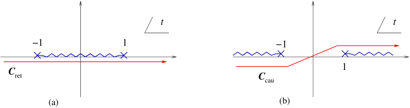
Figure 2: Cuts and integration paths for the ”retarded” (a) and “causal” (b) solutions of eq. (38).

The $U$-part of $\psi_{c}$ can be obtained with a “causal” prescription for the pole shift, as shown in fig. 2b:

$$\psi_{\mathrm{cau}}(\rho) \equiv\frac{\mathrm{i}\mathrm{e}^{\pi\alpha}}{\pi}\int_{-\infty}^{+\infty}\mathrm{d}t\;\mathrm{e}^{\mathrm{i}2\alpha\rho t}\,(t-1+\mathrm{i}0)^{\mathrm{i}\alpha-1}(t+1-\mathrm{i}0)^{-\mathrm{i}\alpha-1}$$

$$=\frac{\mathrm{i}}{\pi}\int_{-\infty-\mathrm{i}0}^{+\infty+\mathrm{i}0}\mathrm{d}t\;\frac{\mathrm{e}^{\mathrm{i}2\alpha\rho t}}{t^{2}-1}\left(\frac{1-t}{1+t}\right)^{\mathrm{i}\alpha}$$

$$=z\mathrm{e}^{-z/2}\left[\frac{\mathrm{i}}{\pi}\Gamma(\mathrm{i}\alpha)\sinh(\pi\alpha)U(1+\mathrm{i}\alpha,2,z)+\mathrm{e}^{-\pi\alpha}\Theta(\mathrm{i}z)F(1+\mathrm{i}\alpha,2,z)\right]\;.$$ (41)

The Coulomb wave function (33) is now easily obtained as a linear combination of the retarded and causal solutions:

$$\psi_{c} =N_{c}\frac{\mathrm{i}\pi}{\Gamma(\mathrm{i}\alpha)\sinh(\pi\alpha)}\left[\cosh(\pi\alpha)\psi_{\mathrm{ret}}-\psi_{\mathrm{cau}}\right]$$

$$=\frac{(4\mathrm{i}\alpha L^{2})^{\mathrm{i}\alpha}}{\Gamma(\mathrm{i}\alpha)\sinh(\pi\alpha)\cosh(\pi\alpha)}\left(\int_{C_{\mathrm{cau}}}-\cosh(\pi\alpha)\mathrm{e}^{\pi\alpha}\int_{C_{\mathrm{ret}}}\right)\frac{\mathrm{e}^{\mathrm{i}2\alpha\rho t}}{t^{2}-1}\left(\frac{1-t}{1+t}\right)^{\mathrm{i}\alpha}\;\mathrm{d}t\;.$$ (42)

A convenient representation of $\psi_{c}$ with a branch cut at finite $t$ can be obtained by means of the relation

$$\left(\frac{1-t}{1+t}\right)^{\mathrm{i}\alpha}=\mathrm{e}^{\mathrm{sign}(\Im t)\,\pi\alpha}\left(\frac{t-1}{t+1}\right)^{\mathrm{i}\alpha}\;,$$ (43)

and is given by

$$\psi_{c}=\frac{(4\mathrm{i}\alpha L^{2})^{\mathrm{i}\alpha}}{\Gamma(\mathrm{i}\alpha)\cosh(\pi\alpha)}\left(-\int_{-\infty-\mathrm{i}\epsilon}^{1}+\int_{1}^{+\infty}\right)\frac{\mathrm{e}^{\mathrm{i}2\alpha\rho t}}{t^{2}-1}\left(\frac{t-1}{t+1}\right)^{\mathrm{i}\alpha}\;\mathrm{d}t\;.$$ (44)

It is straightforward at this point to perform the gaussian integration in eq. (28)

$$\int\frac{\mathrm{d}\rho}{(\pi b^{2}/\mathrm{i}\alpha)^{1/2}}\;\mathrm{e}^{-\mathrm{i}\alpha(\rho^{2}/b^{2}+b^{2})}\mathrm{e}^{\mathrm{i}2\alpha\rho t}=\mathrm{e}^{\mathrm{i}\alpha b^{2}(t^{2}-1)}$$ (45)

yielding the $b$-dependent tunneling amplitude

$$\mathcal{T}(b,\alpha) =\frac{(4\mathrm{i}\alpha L^{2})^{\mathrm{i}\alpha}}{\Gamma(\mathrm{i}\alpha)\cosh(\pi\alpha)}\left(-\int_{-\infty-\mathrm{i}\epsilon}^{1}+\int_{1}^{+\infty}\right)\frac{\mathrm{e}^{\mathrm{i}\alpha b^{2}(t^{2}-1)}}{t^{2}-1}\left(\frac{t-1}{t+1}\right)^{\mathrm{i}\alpha}\;\mathrm{d}t$$ (46a)

$$=\frac{(4\mathrm{i}\alpha L^{2})^{\mathrm{i}\alpha}}{\Gamma(\mathrm{i}\alpha)\cosh(\pi\alpha)}\left(\int_{-\infty-\mathrm{i}\epsilon}^{1}-\int_{1}^{+\infty}\right)b^{2}t\left(\frac{t-1}{t+1}\right)^{\mathrm{i}\alpha}\mathrm{e}^{\mathrm{i}\alpha b^{2}(t^{2}-1)}\;\mathrm{d}t\;,$$ (46b)

where an integration by part has been performed in the last step.

At $b=0$, the transition amplitude can be computed by noting that the integral $\int_{-\infty-\mathrm{i}\epsilon}^{1}+\int_{1}^{+\infty}$ of the integrand (46a) can be closed on the lower half-plane and gives a vanishing result. Therefore

$$\mathcal{T}(0,\alpha)=\frac{(4\mathrm{i}\alpha L^{2})^{\mathrm{i}\alpha}}{\Gamma(\mathrm{i}\alpha)\cosh(\pi\alpha)}2\int_{1}^{+\infty}\frac{(t-1)^{\mathrm{i}\alpha-1+0}}{(t+1)^{\mathrm{i}\alpha+1}}\;\mathrm{d}t=\frac{(4\mathrm{i}\alpha L^{2})^{\mathrm{i}\alpha}}{\Gamma(\mathrm{i}\alpha)\cosh(\pi\alpha)}\,\frac{1}{\mathrm{i}\alpha}$$ (47)

which correctly reproduces the result in eq. (34).

On the other hand, at $b>0$, the integral $\int_{1}^{+\infty}$ is exponentially suppressed with respect to $\int_{-\infty-\mathrm{i}\epsilon}^{1}$. This can be shown by bending the paths of the two contributions as shown in fig. 3 and by noting that the order of magnitude of the integrand is $\sim\mathrm{e}^{-\pi\alpha}$ above the cut and $\sim\mathrm{e}^{+\pi\alpha}$ below it.

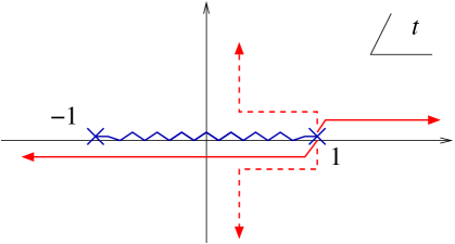
Figure 3: Integration paths of eq. (46) (solid lines). The corresponding deformed paths (dashed lines) are such that the lower one dominates $\mathcal{T}$ while the contribution stemming from the upper one is strongly suppressed.

3.3 Evaluating absorption at quantum level

In order to take into account multi-graviton emission, we consider the $S$-matrix in eq. (17) with non-vanishing values of the absorption parameter $y=2Y/\pi$ which effectively takes into account the longitudinal phase space of gravitons. In the following, we consider $y$ as a free parameter ($0<y<\infty$), independent of $\alpha\equiv Gs/\hbar$, which can vary from small to large values according to the effective transverse mass of the light particles being emitted. We note, however, as anticipated in sec. 2.1, that the dynamics (sec. 6) will normally introduce correlations, and the latter can depress or emphasize some regions of rapidity phase space, as it happens for the case of energy conservation [11], thus providing $\alpha$- and $b$-dependent constraints on the range of possible $y$’s.

For $y\neq 0$, the tunneling amplitude with absorption $\mathcal{T}(b,\alpha,y)$ is again given by eq. (25), but in this case the time-dependent wave function (24) is determined by a non-unitary evolution operator $\mathcal{U}_{y}(\tau,\infty)$, due to the fact that the Hamiltonian operator of the quantum system is no longer hermitian, as it should in order to describe absorptive effects due to inelastic production.

In fact, the absorption term in eq. (15) adds an imaginary part to the kinetic term in the Lagrangian (18) and formally changes the definition of the Hamiltonian and of the quantization condition in terms of a new parameter $\tilde{\alpha}\equiv\alpha(1-\mathrm{i}y)$:

$$\tilde{H}=\tilde{\alpha}\left(\dot{\hat{\rho}}\,^{2}-1\right)+\frac{\alpha}{\hat{\rho}}\Theta(\tau-b^{2})\;,\qquad[\hat{\rho},\dot{\hat{\rho}}]=\frac{\mathrm{i}\hbar}{2\tilde{\alpha}}\;,\qquad\tilde{\alpha}\equiv\alpha(1-\mathrm{i}y)\;.$$ (48)

A simple way to take into account such changes is to solve the evolution equation for the wave-function $\langle t|\psi(\tau)\rangle\equiv\tilde{\psi}(t;\tau)$ directly in the momentum representation (35) in which $\dot{\hat{\rho}}=t$ is diagonal. We simply obtain

$$\mathrm{i}\frac{\partial}{\partial\tau}\tilde{\psi}(t;\tau)=\left[\tilde{\alpha}(t^{2}-1)+\alpha\Theta(\tau-b^{2})\left(\frac{\mathrm{i}}{2\tilde{\alpha}}\frac{\partial}{\partial t}\right)^{-1}\right]\tilde{\psi}(t;\tau)\;.$$ (49)

For $\tau>b^{2}$, the evolution involves the Coulomb-type Hamiltonian with zero energy (due to the boundary condition $\dot{\rho}(\infty)=1$) and we get the solution

$$\tilde{\psi}(t;\tau)=\left(\frac{t-1}{t+1}\right)^{\mathrm{i}\alpha}\frac{1}{t^{2}-1}N(\alpha,y)\;,\qquad(\tau>b^{2})\;,$$ (50)

where the normalization factor $N(\alpha,y)$ will be fixed later on. On the other hand, for $\tau\leq b^{2}$ we have just free evolution,

$$\mathrm{i}\frac{\partial}{\partial\tau}\log\tilde{\psi}(t;\tau)=\tilde{\alpha}(t^{2}-1)\;,$$ (51)

yielding

$$\tilde{\psi}(t;\tau)=N(\alpha,y)\left(\frac{t-1}{t+1}\right)^{\mathrm{i}\alpha}\frac{1}{t^{2}-1}\mathrm{e}^{\mathrm{i}\alpha(1-\mathrm{i}y)(1-t^{2})(\tau-b^{2})}\;,\qquad(\tau\leq b^{2})$$ (52)

and therefore

$$\psi(\rho,\tau)=N(\alpha,y)\int\mathrm{d}t\;\left(\frac{t-1}{t+1}\right)^{\mathrm{i}\alpha}\frac{1}{t^{2}-1}\mathrm{e}^{\mathrm{i}\alpha(1-\mathrm{i}y)(1-t^{2})(\tau-b^{2})}\mathrm{e}^{\mathrm{i}2\alpha(1-\mathrm{i}y)\rho t}\;.$$ (53)

By then setting $\rho=0$ and $\tau=0$, we get the desired result

$$\psi(0,0)=N(\alpha,y)\int\mathrm{d}t\;\left(\frac{t-1}{t+1}\right)^{\mathrm{i}\alpha}\frac{1}{t^{2}-1}\mathrm{e}^{\mathrm{i}\alpha b^{2}(1-\mathrm{i}y)(t^{2}-1)}\;,$$ (54)

which is consistent at $y=0$ with the representation (46a), and differs from it at $y>0$ by the replacement $b^{2}\to\tilde{b}^{2}\equiv b^{2}(1-\mathrm{i}y)$.

It remains to determine the proper integration path(s) and the normalization factor $N$ in eq. (54). In the $y=0$ limit we require $N(\alpha,0)$ and the integration path to agree with eq. (46a). By continuity, the integration path at $y>0$ is obtained by rotating the original one in counter clock-wise direction, as shown in fig. 4a, in such a way to remain in the convergence sectors of $\mathrm{e}^{\mathrm{i}\alpha b^{2}(1-\mathrm{i}y)t^{2}}$, given by $\phi/2<\arg(\pm t)<\phi/2+\pi/2$ where $\phi\equiv-\arg(1-\mathrm{i}y)>0$.

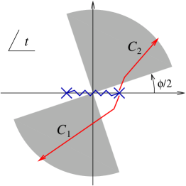
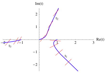
Figure 4: (a) Convergence sector and integration paths for the $t$-representation of the tunneling amplitude including absorption. (b) Position of the saddle points for $y=0.5$ in the complex $t$-plane. As $b$ approaches infinity, the three saddle points approach the real axis at the points $-1$, $0$ and $1$. The short red lines indicate the steepest descent directions for $b=1/4$, $1/2$, $1$ and $2$.

The normalization factor is fixed by the requirement of unitarity at large $b$, namely
$\lim_{b\to\infty}|\mathcal{T}(b,\alpha,y)|=1$, and can be determined as follows. Firstly, one notes that the integrals along $C_{1}$ and $C_{2}$ are dominated by saddle points at $t_{1}$ and $t_{2}$ respectively, with $t_{1}\to 1$ and $t_{2}\to 0$ as $b\to\infty$, as shown in fig. 4b. The saddle point condition is given by $b^{2}(1-\mathrm{i}y)t_{k}(1-t_{k}^{2})=1$ and one has (cfr. app. A of [5])

$$\int_{C_{1}+C_{2}}\mathrm{d}t\; \left(\frac{t-1}{t+1}\right)^{\mathrm{i}\alpha}\frac{1}{t^{2}-1}\mathrm{e}^{\mathrm{i}\alpha b^{2}(1-\mathrm{i}y)(t^{2}-1)}$$

$$\simeq\sum_{k=1}^{2}(-1)^{k-1}t_{k}\left(\frac{t_{k}-1}{t_{k}+1}\right)^{\mathrm{i}\alpha}\mathrm{e}^{-\mathrm{i}\alpha/t_{k}}\sqrt{\frac{\pi}{\mathrm{i}\alpha t_{k}(3t_{k}^{2}-1)}}$$

$$\xrightarrow{b\to\infty}\mathrm{e}^{\pi\alpha}\sqrt{\frac{\pi}{2\mathrm{i}\alpha}}\left(4\mathrm{e}b^{2}(1-\mathrm{i}y)\right)^{-\mathrm{i}\alpha}-\mathrm{e}^{-\pi\alpha}\sqrt{\frac{\mathrm{i}\pi}{\alpha b^{2}(1-\mathrm{i}y)}}\mathrm{e}^{-\mathrm{i}\alpha b^{2}}\mathrm{e}^{-\alpha b^{2}y}$$ (55)

Secondly, one observes that at large $b$ (and even more at large $\alpha$) the contribution of the saddle point $t_{2}$ is suppressed with respect to the contribution from $t_{1}$, therefore

$$T(b,\alpha,y)\simeq N(\alpha,y)\,\mathrm{e}^{\pi\alpha}\sqrt{\frac{\pi}{2\mathrm{i}\alpha}}\left(4\mathrm{e}b^{2}(1-\mathrm{i}y)\right)^{-\mathrm{i}\alpha}\;,\qquad(b\to\infty)\;.$$ (56)

Finally, from the unitarity requirement, which can be also written as a “Coulomb phase” normalization condition

$$\lim_{b\to\infty}\frac{\mathcal{T}(b,\alpha,y)}{\mathcal{T}(b,\alpha,0)}=1\;,$$ (57)

we obtain $N(\alpha,y)(1-\mathrm{i}y)^{-\mathrm{i}\alpha}=N(\alpha,0)$, and we conclude that the elastic $S$-matrix (or, the tunneling amplitude including absorption) is given by

$$\mathcal{T}(b,\alpha,y)=\frac{(4\mathrm{i}\alpha L^{2})^{\mathrm{i}\alpha}(1-\mathrm{i}y)^{\mathrm{i}\alpha}}{\Gamma(\mathrm{i}\alpha)\cosh(\pi\alpha)}\int_{C_{1}+C_{2}}\frac{\mathrm{e}^{\mathrm{i}\alpha b^{2}(1-\mathrm{i}y)(t^{2}-1)}}{t^{2}-1}\left(\frac{t-1}{t+1}\right)^{\mathrm{i}\alpha}\;\mathrm{d}t\;.$$ (58)

Note that the factor $|N(\alpha,y)|=\mathrm{e}^{\alpha\phi}$ is needed to cancel the extra large-$b$ suppression (56), and thus enhances the $b=0$ amplitude $\mathrm{e}^{-\alpha(\pi-\phi)}$, which increases to $\mathrm{e}^{-\pi\alpha/2}$ for $y\to\infty$.

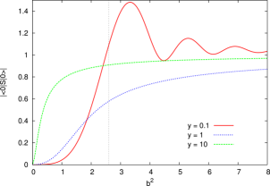
Figure 5: Transition amplitude at $\alpha=5$ for three values of the absorption parameter y. Large-$b$ behaviour in linear scale (a); small-$b$ behaviour in logarithmic scale (b). The vertical dashed line in (a) shows the critical value $b_{c}$; the horizontal dashed lines in (b) are the boundaries $\sim[\mathrm{e}^{-\pi\alpha},\mathrm{e}^{-\pi\alpha/2}]$ of the $b\to 0$ limits of the amplitude for $y$ ranging from zero to infinity.

In fig. 5 we have plotted the dependence on the impact parameter $b$ of the elastic $S$-matrix, for three values of the inelasticity $y$. For small $y$’s ($y=0.1$ say) there are some oscillations, due to the interference of the saddle points $t_{1}$ and $t_{2}^{I\!I}$ (on the second $t$-sheet reached across the $[-1,1]$ cut) for the contour $C_{1}$. This shows that the elastic unitarity bound is marginally overcome if $y$ is too small. In all other cases (with sizeable values of $y$), we observe that the v.e.v. of $S$ is below 1 thus satisfying the elastic unitarity bound, and tends to 1 for large $b$ without oscillations. This is evidence of only one saddle point ($t_{1}$) effectively contributing to the integral for sizeable values of $y$ and $b$. At larger $y$, fixed $b$, the vacuum-to-vacuum amplitude is less suppressed than at smaller $y$, and the small-$b$ suppression of the tunneling amplitude is delayed towards smaller values of $b<b_{c}$. Roughly, the turning point is at values of $b$ of order $b_{c}(1+y^{2})^{-1/4}$, thus extending to values of $b$ smaller than $b_{c}$ the validity of the perturbative behaviour. Nevertheless, in the $b\to 0$ limit, the amplitude tends to the (non-perturbative) constant limit $\mathrm{e}^{-\alpha(\pi-\phi)}$, between $\mathrm{e}^{-\pi\alpha}$ ($y\to 0$) and $\mathrm{e}^{-\pi\alpha/2}$ ($y\to\infty$).

We thus see the emergence of two absorptive regimes, according to the values of $y$. In the very small-$y$ regime, quantum interference is important, in particular for small $b-b_{c}$ the saddle points $t_{1}$ and $t_{2}^{I\!I}$ collide and interfere by confirming the critical role of $b_{c}$, but leading to an analytic $S$-matrix at $b=b_{c}$, as explained in [5]. On the other hand, for sizeable to large values of $y$ only one saddle point dominates and the perturbative and tunneling regimes are hardly distinguishable at $b\simeq b_{c}$, the perturbative behaviour with small absorption being extended to smaller values of $b$. However, we shall see in the following that including inelastic channels will make things even, by restoring the role of $b=b_{c}$ for unitarity purposes, for any values of $y$.

4 Inelastic processes and $\boldsymbol{S}$-matrix eigenstates

So far we have analyzed the $S$-matrix in the elastic channel, deriving in eq. (58) an explicit expression for the probability amplitude

$$\mathcal{T}=\langle 0|S|0\rangle$$ (59)

which represents, in this simplified model (15) of transplanckian scattering, the string-string scattering amplitude without graviton emission (a state represented by the graviton vacuum $|0\rangle$).

We found that starting from the elastic channel (the vacuum state), our quantum calculation provides absorption for any value of the impact parameter $b$, and that for $b<b_{c}$ (critical value) the tunneling absorption persists even if the graviton-emission phase-space parameter $y$ were set to zero. This means that the contribution to the $S$-matrix of quite inelastic states is essential to possibly recover unitarity.

In this section we investigate the issue of unitarity of our model (5) from various points of view.

4.1 Eigenstates and eigenvalues of the $\boldsymbol{S}$-matrix

A convenient way to determine whether or not the $S$-matrix is a unitary operator is to look for its eigenvalues. Due to the particularly simple form of our $S$-matrix as (superposition of) coherent state operators in the graviton Fock space, it turns out that the $S$-matrix eigenstates are functional Fourier transforms of the Fock-space coherent states. In detail, we define the generic graviton-coherent-state

$$|\eta(\tau)\rangle\equiv\mathrm{e}^{-\frac{1}{2}(\eta^{*},\eta)}\exp\left\{\int\frac{\mathrm{d}^{2}\boldsymbol{x}}{\sqrt{\pi}}\;a^{\dagger}(\boldsymbol{x})\eta(\boldsymbol{x}^{2})\right\}|0\rangle$$ (60)

where $\eta(\tau)$ is the distribution function of gravitons in the radial coordinate $\tau\equiv\boldsymbol{x}^{2}$, and we have introduced the scalar product notation $(\eta,\zeta)\equiv\int_{0}^{\infty}\eta(\tau)\zeta(\tau)\;\mathrm{d}\tau$. Then, by means of a (normalized) functional integration in $\tau$-space we introduce the Fourier transform of coherent-states

$$|\{\omega(\tau)\}\rangle\equiv\mathrm{e}^{\frac{1}{4}(\omega,\omega)}\int[\mathcal{D}\zeta(\tau)]\;\mathrm{e}^{-\mathrm{i}(\omega,\zeta)}|\mathrm{i}\zeta\rangle\;,$$ (61)

which are parameterized by the radial function $\omega(\tau)$. It is straightforward to prove (app. A) that such states are eigenstates of the $S$-matrix (5)

$$S|\{\omega(\tau)\}\rangle =\int[\mathcal{D}\rho(\tau)]\;\mathrm{e}^{-\mathrm{i}\int L(\rho,\tau)\;\mathrm{d}\tau+\mathrm{i}(\omega,\delta_{\rho})}|\{\omega(\tau)\}\rangle\equiv\mathrm{e}^{\mathrm{i}{\cal A}[\omega;b,\alpha]}|\{\omega(\tau)\}\rangle\;,$$ (62)

$$\delta_{\rho}(\tau) \equiv\sqrt{2\alpha y}\big{(}1-\dot{\rho}(\tau)\big{)}\;,$$ (63)

with eigenvalues $\mathrm{e}^{\mathrm{i}{\cal A}[\omega]}$. Furthermore, the $\omega$-states are orthonormal in the continuum spectrum and are argued to be complete in the Fock space (app. A).

The actual evaluation of the $S$-matrix eigenvalues involves the path-integral in eq. (62), whose action differs from the vacuum one by the $\omega$-dependent contribution $(\omega,\delta_{\rho})$. At the semiclassical level it is easy to derive the modified equation of motion

$$2\ddot{\rho}-\frac{\Theta(\tau-b^{2})}{\rho^{2}}=-\sqrt{\frac{2y}{\alpha}}\dot{\omega}(\tau)$$ (64)

in which $\dot{\omega}$ plays the role of external force, depending on the given eigenvalue function $\omega(\tau)$.

In the strict $\dot{\omega}=0$ limit we are left with the vacuum state equation characterized by the usual matching condition (in the $y=0$ limit)

$$\frac{1}{b^{2}}=t_{b}(1-t_{b}^{2})\;,\qquad\left(t_{b}=\dot{\rho}(b^{2})\right)$$ (65)

and by $\rho(b^{2})=t_{b}\,b^{2}=\rho_{b}\equiv 1/(1-t_{b}^{2})$. Real-valued solutions with $\rho(0)=0$ and $\dot{\rho}(\infty)=1$ exist only for $b\geq b_{c}$, with $b_{c}^{2}=3\sqrt{3}/2$. For $b<b_{c}$ there are complex solutions, yielding a complex-valued semiclassical eigenvalue and a calculable absorption, so that $|S(\omega=0;b,\alpha)|<1$ for $b<b_{c}$. This simple observation has the consequence that the $S$-matrix violates unitarity, to some extent, for values of the impact parameter smaller than the critical value $b_{c}$. This means that the $y$-independent $b_{c}$ separates the perturbative unitary regime ($b>b_{c}$) from a regime where a unitarity defect is possible ($b<b_{c}$), rather than separating absorptive and tunneling regimes of the elastic channel, as discussed previously. The actual unitarity violation for $b<b_{c}$ is dependent on the relative weight of the small-$\omega$ states in physical matrix elements and is the subject of the following analysis.

On the other hand, it is essential to note that, if $\dot{\omega}(\tau)$ is allowed to take properly chosen (large) values, then real-valued solutions of (64) turn out to exist for all $b$’s, thus yielding a real ${\cal A}(\omega)$ and a unitary eigenvalue with $|S(\omega)|=1$. A large class “$R$” of such solutions is found by setting

$$\omega_{R}(\tau)=\sqrt{\frac{2\alpha}{y}}\left[-\frac{\Delta}{1-\Delta}(1-\dot{\rho}_{R})\Theta(\tau-b^{2})+(B-\dot{\rho}_{R})\Theta(b^{2}-\tau)\right]\;,$$ (66)

where $\Delta\in\mathbb{R}$ is arbitrary, $\rho_{R}$ is the semiclassical solution itself and $B=(t_{b}-\Delta)/(1-\Delta)$ by the continuity requirement on $\omega$ and $\dot{\rho}_{R}$ at $\tau=b^{2}$. By replacing the ansatz (66) in the equation of motion (64) we find in the $\tau>b^{2}$ region

$$2\ddot{\rho}_{R}=\frac{1-\Delta}{\rho_{R}^{2}}\qquad(\tau>b^{2})\;,$$ (67)

while, for $\tau<b^{2}$, we can take $\rho(\tau)$ to be any function with continuous $\rho$ and $\dot{\rho}$ and finite $\ddot{\rho}$, satisfying $\rho(0)=0$, and matching the Coulomb-like solution in eq. (67) at $\tau=b^{2}$, i.e., satisfying $\dot{\rho}(b^{2})=t_{b}$ and $\rho(b^{2})=\rho_{b}\equiv(1-\Delta)/(1-t_{b}^{2})$. This is an infinite-parameter set of functions, since the Taylor coefficients $\rho^{(n)}(\bar{\tau})$ ($0<\bar{\tau}<b^{2}$) for $n\geq 3$ are arbitrary.

We see that the effect of the parameter $\Delta$ occurring in the external force $\dot{\omega}_{R}$ provided by the eigenstate is to renormalize the Coulomb coupling in eq. (67) by the factor $1-\Delta$, so that it may become less repulsive for $0\leq\Delta<1$ and even attractive for $\Delta>1$. The main point is, though, that eq. (64) is identically satisfied by the ansatz (66) by setting no constraints on $\ddot{\rho}(\tau)$ in the $0\leq\tau<b^{2}$ region, so that the external force allows automatically real-valued solutions for any value of $b$. Therefore, for any $b$, eq. (66) yields a family of eigenstates of the $S$-matrix with unitary eigenvalues depending on an infinite set of parameters: two of them ($\Delta$ and $t_{b}$) characterize the Coulomb problem in eq. (67), and an infinity of them (the higher-order Taylor coefficients) span the set of functions $\rho(\tau)$ for $0<\tau<b^{2}$.

We stress the point that the very existence of such unitary eigenstates is a consequence of the quantum structure of the $S$-matrix (15) in which the field $\rho(\tau)$ is allowed to fluctuate until it reaches the relevant solution $\rho_{R}$ of (64). The only problem of such states $\{\omega_{R}\}$ is that their overlap with the vacuum is suppressed by the factor

$$|\langle\{\omega_{R}\}|0\rangle|^{2}=\mathrm{e}^{-\frac{1}{2}(\omega_{R},\omega_{R})}\;,$$ (68)

where the exponent is of order $\alpha/y$. Therefore, such states become important only in the $y\gg\alpha$ limit.

We have thus singled out two families of $S$-matrix eigenstates: the small-$\omega$ one which exhibits a critical value $b=b_{c}$, below which no real-valued semiclassical solutions exist and the tunneling phenomenon occurs (with non-unitary eigenvalues), and the large-$\omega$ one, in which an infinite-parameter family of unitary eigenstates exists, characterized by the eigenvalue functions $\omega_{R}(\tau)$ in eq. (66). This shows that unitarity is not an exact property of our quantum model and indicates that unitarity violations, for any given initial state, are determined by the overlap profile of such states on the various eigenstates.

4.1.1 Sum over eigenstates for the elastic channel

Using the vacuum wave functional $\langle\{\omega\}|0\rangle=\mathrm{e}^{-\frac{1}{4}(\omega,\omega)}$ it is easy to construct, by eq. (62), the matrix element

$$\langle 0|S|\{\omega\}\rangle=\langle\{\omega\}|S|0\rangle=\mathrm{e}^{-\frac{1}{4}(\omega,\omega)}\mathrm{e}^{\mathrm{i}{\cal A}(\omega)}$$ (69)

and then, by summing over the complete set $|\{\omega(\tau)\}\rangle$, the v.e.v.

$$\langle 0|S|0\rangle =\int[\mathcal{D}\omega]\;\langle 0|S|\{\omega\}\rangle\langle\{\omega\}|0\rangle=\int[\mathcal{D}\omega]\;\mathrm{e}^{-\frac{1}{2}(\omega,\omega)}\mathrm{e}^{\mathrm{i}{\cal A}(\omega)}$$

$$=\int[\mathcal{D}\rho]\;\mathrm{e}^{-\mathrm{i}\int L(\rho,\tau)\;\mathrm{d}\tau-\frac{1}{2}(\delta_{\rho},\delta_{\rho})}\;,$$ (70)

a result already studied in detail in ref. [5] and in the previous sections.

We thus remark that the quadratic $\omega$-integration in eq. (70) introduces explicitly the absorption parameter $y$ in the vacuum equations, via the saddle-point value $\omega_{s}=\mathrm{i}\delta_{\rho}(\tau)=\mathrm{i}\sqrt{2\alpha y}\big{(}1-\dot{\rho}(\tau)\big{)}$. We then recover the equation of motion of the elastic channel

$$2\ddot{\rho}(1-\mathrm{i}y)-\frac{\Theta(\tau-b^{2})}{\rho^{2}}=0$$ (71)

whose solutions are complex for any $b$ value, unlike the $\omega=0$ limit of eq. (64) which admits real-valued solutions for $b>b_{c}$ [2]. A consequence of this feature is that for any $b$ value eq. (71) predicts the non-vanishing absorption of sec. 3.3, which, for $b<b_{c}$, tends to a finite limit even in the $y=0$ limit. Therefore, one has to look in principle at all possible inelastic channels in order to check whether the absorption of the elastic one can be compensated by the unitarity sum.

4.1.2 States approximating the unitarity sum

The simplest approach is to look at the unitarity sum for the $S$-matrix from the point of view of the squared matrix elements in eq. (69) in order to identify the states that maximally contribute to the sum. Since the (quasi)elastic matrix elements are absorbed, and the eigenstates with unitary eigenvalues are suppressed by the overlap with the vacuum state, the overall unitarity defect is a balance of the two absorptive effects just mentioned. A fully quantitative analysis is better done by the method of sec. 5. Here we look at the contribution of the unitary eigenstates $|\{\omega_{R}\}\rangle$ only and this will provide a lower bound to the unitarity sum, as follows

$$\langle 0|S^{\dagger}S|0\rangle=\int[\mathcal{D}\omega]\;|\langle\{\omega\}|S|0\rangle|^{2}\geq\int[\mathcal{D}\omega_{R}]\;|\langle\{\omega_{R}\}|S|0\rangle|^{2}=\int[\mathcal{D}\omega_{R}]\;\mathrm{e}^{-\frac{1}{2}(\omega_{R},\omega_{R})}\;,$$ (72)

where we have used the fact that $|S(\omega_{R})|=1$. Thus the suppression exponent of this lower bound is here provided by the vacuum functional $(\omega_{R},\omega_{R})$.

In order to optimize the lower bound above (72), we look for states that minimize $(\omega_{R},\omega_{R})$ in the sample defined by eq. (66). By imposing stationarity on the infinite set of parameters $\rho^{(n)}(\bar{\tau})$ ($n\geq 3$) we easily find that $\dot{\rho}(\tau)$ must be a constant for $\tau<b^{2}$, and the latter, by continuity, must be $\dot{\rho}(b^{2})=t_{b}$. Therefore, we have the matching condition

$$1-\Delta=b^{2}t_{b}(1-t_{b}^{2})$$ (73)

which corresponds to a Coulomb problem with “charge” $(1-\Delta)$. This allows to replace $\Delta(t_{b})$ in the expression

$$\frac{1}{2}(\omega_{R},\omega_{R}) =\frac{\alpha}{y}\frac{\Delta^{2}}{(1-\Delta)^{2}}\left[\int_{b^{2}}^{\infty}(1-\dot{\rho}_{R})^{2}\;\mathrm{d}\tau+b^{2}(1-t_{b}^{2})\right]$$

$$=\frac{\alpha}{y}\left[\frac{1}{b^{2}}-t_{b}(1-t_{b}^{2})\right]^{2}\frac{b^{2}}{t_{b}^{2}(1+t_{b})}\;.$$ (74)

For $b\geq b_{c}$, this expression has a vanishing minimum with $\Delta=0$, corresponding to unitarity fulfillment, with a slope parameter varying from $(1-t_{b})\sim 1/(2b^{2})$ for $b\gg b_{c}$, to $t_{b}=t_{c}\equiv 1/\sqrt{3}$ for $b=b_{c}$ (as usual). Instead, for $b<b_{c}$, the minimum becomes non-vanishing, with $t_{b}=\bar{t}_{b}$ increasing from $t_{c}$ to $\bar{t}_{b}\sim(b^{2})^{-1/3}\to\infty$ for $b$ decreasing from $b_{c}$ to $0$, according to the law

$$\frac{1}{b^{2}}=\frac{1+3\bar{t}_{b}}{2+3\bar{t}_{b}}\bar{t}_{b}^{\,2}(1+\bar{t}_{b})\;.$$ (75)

Correspondingly, the value of $\Delta$, starting from $\Delta=0$ for $b=b_{c}$, increases towards $\Delta=2$ for $b\to 0$, so that the Coulomb potential becomes eventually attractive. The value of (73) at the minimum becomes

$$\frac{1}{2}(\bar{\omega}_{R},\bar{\omega}_{R})=\frac{4\alpha}{y}\frac{(1-3\bar{t}_{b}^{\,2})^{2}}{\bar{t}_{b}^{\,2}(2+3\bar{t}_{b})(1+3\bar{t}_{b})}\xrightarrow{b\to 0}\frac{4\alpha}{y}\;.$$ (76)

and has the property of vanishing in the $y\to\infty$ limit.

We tentatively conclude that our quantum $S$-matrix is always unitary for $b>b_{c}$ and may be unitary for $b<b_{c}$ also, provided $y/\alpha\to\infty$, the unitarity sum being approximated by the $\omega_{R}$’s as given above. This is due to the fact that $(\omega_{R},\omega_{R})$ becomes small in that limit, and is consistent with the vanishing of the “unitarity action” ${\cal A}_{u}(y\to\infty)\to 0$ that we shall derive in the next section.

5 The unitarity action and its features

5.1 The unitarity action around the vacuum state

As an alternative method, it is possible to check unitarity directly by performing the sum over $S$-matrix eigenstates exactly, at fixed field $\rho(\tau)$. Since the integration over $\omega$ is quadratic, the unitarity sum becomes

$$\langle 0|S^{\dagger}S|0\rangle =\int[\mathcal{D}\omega]\;|\langle\{\omega\}|S|0\rangle|^{2}=\int[\mathcal{D}\omega]\;\mathrm{e}^{-\frac{1}{2}(\omega,\omega)}\mathrm{e}^{-2\Im{\cal A}(\omega)}$$

$$=\int[\mathcal{D}\rho][\mathcal{D}\tilde{\rho}]\;\mathrm{e}^{\mathrm{i}\int[L(\rho)-L(\tilde{\rho})]\;\mathrm{d}\tau-\frac{1}{2}(\delta_{\rho}-\delta_{\tilde{\rho}},\delta_{\rho}-\delta_{\tilde{\rho}})}\equiv\int[\mathcal{D}\rho][\mathcal{D}\tilde{\rho}]\;\mathrm{e}^{\mathrm{i}{\cal A}_{u}}\;,$$ (77)

where we have performed the $\omega$-integration around the saddle point $\omega_{s}=\mathrm{i}(\delta_{\rho}-\delta_{\tilde{\rho}})=\mathrm{i}\sqrt{2\alpha y}(\dot{\tilde{\rho}}-\dot{\rho})$, by introducing the path-integral representation of $S(\omega)$. It is then straightforward to derive the semiclassical equations

$$\begin{cases}2\ddot{\rho}-2\mathrm{i}y(\ddot{\rho}-\ddot{\tilde{\rho}})&=\displaystyle{\frac{\Theta(\tau-b^{2})}{\rho^{2}}}\\[8.61108pt] 2\ddot{\tilde{\rho}}+2\mathrm{i}y(\ddot{\tilde{\rho}}-\ddot{\rho})&=\displaystyle{\frac{\Theta(\tau-b^{2})}{\tilde{\rho}^{2}}}\end{cases}$$ (78)

which govern the unitarity action

$${\cal A}_{u}\equiv-\int L(\rho)-L(\tilde{\rho})+\mathrm{i}\alpha y(\dot{\tilde{\rho}}-\dot{\rho})^{2}\;\mathrm{d}\tau\;.$$ (79)

From eq. (78) we see that, for $b>b_{c}$, real-valued solutions with $\tilde{\rho}(\tau)=\rho(\tau)$ exist — both equations reducing to the elastic one (10) — for which the on-shell unitarity action vanishes, thus implying a unitary $S$-matrix, since, at semiclassical level,

$$\langle 0|S^{\dagger}S|0\rangle_{\mathrm{semicl}}=\mathrm{e}^{\mathrm{i}{\cal A}_{u}}\;.$$ (80)

On the other hand, for $b<b_{c}$, the solutions are necessarily complex and eq. (78) can be satisfied by setting $\tilde{\rho}=\rho^{*}$, thus yielding the equation

$$2\ddot{\rho}+4y\Im\ddot{\rho}=\frac{\Theta(\tau-b^{2})}{\rho^{2}}\;,$$ (81)

which is equivalent to a coupled set of equations for $\rho_{1}\equiv\Re\rho$ and $\rho_{2}\equiv\Im\rho$. Note that, unlike the elastic channel case, the equations (81) do not have an analytic structure in $\rho$; therefore they are to be solved as a coupled set of equations having the form

$$\begin{cases}2\ddot{\rho}_{1}+4y\ddot{\rho}_{2}&=\displaystyle{\Re\frac{1}{\rho^{2}}\Theta(\tau-b^{2})}\\[8.61108pt] 2\ddot{\rho}_{2}&=\displaystyle{\Im\frac{1}{\rho^{2}}\Theta(\tau-b^{2})}\end{cases}$$ (82)

under the boundary conditions

$$\rho_{1}(0)=\rho_{2}(0)=\dot{\rho}_{1}(\infty)-1=\dot{\rho}_{2}(\infty)=0\;.$$ (83)

We note that the unitarity action (79) entering the v.e.v. in eq. (80) can be decomposed into two pieces:

$$i{\cal A}_{u}=2\int\Im L(\rho)\;\mathrm{d}\tau+4\alpha y\int h_{2}^{2}\;\mathrm{d}\tau\;,\qquad(h_{2}=\Im\dot{\rho})\;.$$ (84)

The first piece is related to the contribution of the vacuum channel ($n=0$) to the unitarity sum

$$\langle 0|S^{\dagger}S|0\rangle=\sum_{n}\langle 0|S^{\dagger}|n\rangle\langle n|S|0\rangle\;,$$ (85)

since, by eqs. (4,11),

$$\mathrm{e}^{2\int\Im L(\rho_{c})}\simeq|\langle 0|S|0\rangle|^{2}=\langle 0|S^{\dagger}|0\rangle\langle 0|S|0\rangle$$ (86)

where $\rho_{c}$ is the Coulomb-like solution (12). The second piece $\propto h_{2}^{2}$ can then be roughly interpreted as the contribution to the unitarity sum of the inelastic states, and it will be computed in sec. 5.2.

Some simplification in the discussion of (82) is obtained because of the existence of a constant of motion of energy type. By multiplying the first equation by $\dot{\rho}_{2}$ and the second one by $\dot{\rho}_{1}$ and by summing we easily prove the relation (valid for $\tau\geq b^{2}$)

$$\Im\left((\dot{\rho})^{2}+\frac{1}{\rho}\right)+2y\left(\Im\dot{\rho}\right)^{2}=2\dot{\rho}_{1}\dot{\rho}_{2}-\frac{\rho_{2}}{|\rho|^{2}}+2y(\dot{\rho}_{2})^{2}=0\;,$$ (87)

which roughly corresponds to the imaginary part of the single-channel “energy” $(\dot{\rho})^{2}+1/\rho$ (in the $y=0$ limit).

No additional constant of motion seems to be present, the system appearing to be of dissipative type and thus not integrable analytically. We quote a general expression for the on-shell unitarity action ${\cal A}_{u}$, derived in app. B:

$$\mathrm{i}{\cal A}_{u}(y)=2\alpha\left(2\rho_{2}(\infty)+3\Im\frac{1}{t_{b}}\right)\;.$$ (88)

Here $t_{b}=\dot{\rho}(b^{2})$ and $\rho_{2}(\infty)$ characterize the given solution, but do not appear to be related in closed form, so that no matching condition emerges analytically. Nevertheless, one can argue that $\mathrm{i}{\cal A}_{u}(y)\leq 0$ with positive $y$-derivative and that $\lim_{y\to\infty}{\cal A}_{u}(y)=0$. Indeed, on the basis of the equations of motion one can show (app. B.1) that

$$\mathrm{i}\frac{\mathrm{d}{\cal A}_{u}(y)}{\mathrm{d}y}=4\alpha\int\rho_{2}^{2}(\tau)\;\mathrm{d}\tau>0$$ (89)

and that, for large $y$, $y\rho_{2}(\tau;y)$ reaches a finite limit $R_{2}(\tau)$. As a consequence, in eq. (88) both $\rho_{2}(\infty)$ and $t_{2}\equiv\Im t_{b}$ are of order $1/y$. It follows that $|{\cal A}_{u}|=\mathcal{O}\left(\alpha/y\right)$, and thus vanishes in the $y\to\infty$ limit.

5.2 Numerical results

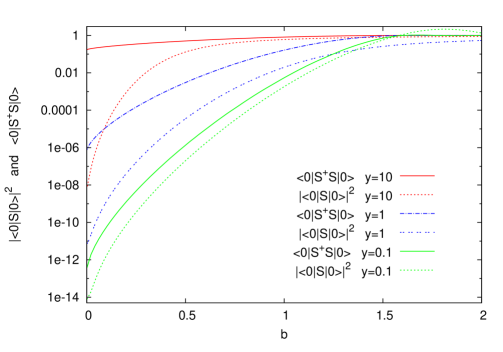
Figure 6: Comparison of the quantum v.e.v. squared of the $S$-matrix (dashed lines) with the semiclassical v.e.v. of the $S^{\dagger}S$ operator (solid lines) for $\alpha=5$ and various values of the absorption parameter y.

We have solved numerically the evolution equations (82) for $(\rho_{1},\rho_{2})$, and we have obtained the unitarity action (88) and the semiclassical vacuum-expectation value of $S^{\dagger}S$ (80) for different values of $y$. In fig. 6 we show our results for $\alpha=5$, $y=0.1,\,1,\,10$, and compare them to the elastic quantum $S$-matrix squared $|\langle 0|S|0\rangle|^{2}=\langle 0|S^{\dagger}|0\rangle\langle 0|S|0\rangle$ which gives the vacuum-channel contribution to the unitarity sum (85). We shall refer to the solutions for $|\langle 0|S|0\rangle|^{2}$ as “exclusive” and to those of $\langle 0|S^{\dagger}S|0\rangle$ as “inclusive” over the inelastic states.

We note that, apart from the unphysical overshoot $|\langle 0|S|0\rangle|>1$ of the transition amplitude at small-$y$ and $b\gtrsim b_{c}$, the inequality $|\langle 0|S|0\rangle|^{2}\leq|\langle 0|S^{\dagger}S|0\rangle|$ is always satisfied. In the small-$y$ limit, inelastic effects are pretty small, in the sense that $|\langle 0|S|0\rangle|^{2}\sim|\langle 0|S^{\dagger}S|0\rangle|$. This reflects the fact that $\rho_{i}(\tau,y)$ coincide with the vacuum solutions in the $y\to 0$ limit (10). Correspondingly, there is a sizeable unitarity violation for $b<b_{c}\simeq 1.6$, inelastic effects providing corrections of relative order $\mathcal{O}\left(y\right)$.

On the other hand, for large values of $y$, inelastic effects are very important, and the $S$-matrix is approximately unitary. In this case, the inclusive solutions are markedly different from the exclusive ones. The latter scale as $\dot{\rho}(b^{2},\tau,y)=\dot{\rho}\big{(}b^{2}(1-\mathrm{i}y),\tau(1-\mathrm{i}y),0)$ and thus are peaked around $\tau\sim 1/y$, with $b^{2}\sim b_{c}^{2}/y$, as roughly seen in fig. 6 so that the tunneling regime is displaced towards smaller values of $b$. This implies in particular that the inelastic weight [cfr. eq. (84)] $y\int h_{2}^{2}\;\mathrm{d}\tau=\mathcal{O}\left(1\right)$ thus showing the importance of inelastic states yielding a finite (non-vanishing) contribution to the unitarity sum (85) in the large-$y$ limit. The inclusive solutions, instead, have $h_{1}\sim\mathcal{O}\left(1\right)$ around $\tau=1$ and $h_{2}\sim\mathcal{O}\left(1/y\right)$ everywhere, yielding a “critical” behaviour around $b\sim b_{c}$, as expected. Since $h_{2}$ is small for large $y$ values, this implies that the on-shell unitarity action scales as $\alpha/y$, yielding small unitarity violations in this limit (figs. 6,7).

The unitarity action is compared in fig. 7 with the unitarity sum (72,76) provided in the previous section. We see that the latter is a good approximation to the unitarity action for large $y$’s, thus providing some understanding of the coherent states dominating the unitarity sum (85), with the corresponding inelasticity $y$.

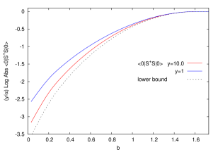
Figure 7: Comparison of the unitarity action (solid lines) with the unitarity bound estimates (76) (dashed lines) for $\alpha=5$ and various values of the absorption parameter $y$. On the left we observe that the unitarity violation for $b<b_{c}\simeq 1.6$ vanishes for increasing values of $y$. On the right, we see that $y$ times the unitarity action tends to a finite limit, which is closely bounded from below by the estimate (76).

At this point, it becomes important to look at the $y\to\infty$ model, which is unitary. Since $b_{c}^{2}(y)$ scales as $b_{c}^{2}(0)/y$, unitarity effects are mostly seen in the small-$b$ region, as illustrated in fig. 6. We see that for large $y$’s inelastic effects indeed fill the unitary defect. Note that $|\langle 0|S|0\rangle|\sim\mathrm{e}^{-\pi\alpha/2}$ in this case (instead of $|\langle 0|S|0\rangle|\sim\mathrm{e}^{-\pi\alpha}$ at $y=0$), thus showing that inelastic effects compensate a finite unitarity defect around $b=0$, consistently with the previous estimate of $y\int h_{2}^{2}\;\mathrm{d}\tau$, providing the order of magnitude of such effects.

6 Discussion

We have presented here a rather comprehensive study of a quantum extension of the ACV gravitational $S$-matrix, both for the elastic matrix element (including absorption) and for the inelastic ones. We have thus been able to provide an analysis of the unitarity problem in the classical collapse region.

A striking outcome of the paper is that our $S$-matrix model satisfies inelastic unitarity for all values of $b$ in the large-$y$ limit $y\gg\alpha\gg 1$. We all know how difficult it is to check unitarity, even in well-known theories where no puzzling classical behaviour is present. Therefore, this result is a quite non-trivial one and encourages us to further investigate the large-$y$ model in detail in order to understand the features of the inelastic production which is able to compensate the exponential tunneling suppression in the small-$b$ region.

A key role, in recovering unitarity, is played by the quantum structure of our $S$-matrix, which allows field fluctuations to build up a class of unitary eigenstates, as explained in sec. 4.1. Such states, characterized by strong fields and small vacuum overlap at finite $y$’s, become actually dominant in the $y\gg\alpha$ limit and turn out to saturate the unitarity sum.

On the other hand, the regime $y\gg\alpha=Gs/\hbar$ appears to be disfavoured for $b<b_{c}$ on the basis of energy conservation and absorptive corrections [11], because for $b\sim R$ emitted gravitons have a somewhat hard transverse mass $\sim\hbar/R$, finally restricting $y$ to be at most $\mathcal{O}\left(\log\alpha\right)$ and actually $\mathcal{O}\left(1\right)$ in the classical collapse region. This means that the unitarity defect that we find for finite $y$’s seems to be the normal feature predicted by our model in the physically acceptable range of $y$’s. An interesting point is that — as we noted in sec. 5 — it is a defect and not an overflow. A possible interpretation of that would be that, in our quantum model, some information loss does show up in the classical collapse region.

However, we do not really believe the unitarity defect of our model to be a possible feature of a consistent quantum gravity theory. We rather think that some of the approximations of string-gravity theory being used in building up the model were inadequate.

Perhaps the weakest point of our model is the use of an uncorrelated coherent state to represent inelastic production in the $S$-matrix for any given field $h(\tau)$. From the original derivation [2], we know that correlations are down by a power of $y$ (actually, a power of $\alpha y$) with respect to uncorrelated emissions. This hierarchy in $y$ could perhaps provide a rationale for the need of a large-$y$ regime to recover unitarity. Furthermore, the existence of correlations could provide a non-linear coherent state, and thus a sort of “condensation” field which could change considerably the analysis of saddle-points in the strong-field configurations and thus provide a mechanism for recovering unitarity. We note that this non-linearity is to some extent predictable from the diagrammatic approach of [2], based on the multi-H diagrams of fig. 1.

We further mention the fact that our quantization procedure keeps frozen the longitudinal space-time structure of the shock-wave. This also is a weak point, and correcting for it — although much more difficult — could provide again further non-linearities in the reduced action and in the $S$-matrix coherent state.

A different way of thinking is to believe that — associated to the classically collapsing states — there are new quantum states, perhaps bound states, which could contribute to the unitarity sum even if the explicit phase-space parameter $y$ were set to zero. We have nothing in principle against this point of view, we only find it difficult to implement it in a predictive way.

To sum up, our investigation of the quantum reduced-action model has led, in part, to a conclusive answer, by exhibiting a unitary version of the model in the (somewhat formal) large-$y$ limit. Future developments include the understanding of the inelastic production of the unitary model which is calculable within our approach. Furthermore, in order to possibly achieve unitarity at finite values of $y$, we think we need improvements of the model itself, probably in the direction of correlated emission, which looks important at finite $y$’s in the classical collapse region.

Appendix A Eigenstates of the $\boldsymbol{S}$-matrix

In this appendix we determine a set of eigenstates of the quantum $S$-matrix, and argue that such set is complete in the Fock-space of gravitons.

The basic ideas are taken from the simpler analogue of a one-dimensional harmonic oscillator with destruction and creation operators $a$ and $a^{\dagger}$ with the usual commutation relation $[a,a^{\dagger}]=1$. The bare-bone structure of the $S$-matrix (5) is in this case

$$S=\mathrm{e}^{\mathrm{i}\Omega}\;,\qquad\Omega\equiv a+a^{\dagger}\;,$$ (90)

where we note that $\Omega$ is proportional to the position operator. An eigenvector $|\{\omega\}\rangle$ of $\Omega$ (and therefore of $S$) with eigenvalue $\omega\in\mathbb{R}$ can be formally found by applying to any state $|\psi\rangle$ the operator $\delta(\Omega-\omega)$:

$$\Omega[\delta(\Omega-\omega)|\psi\rangle]=\omega[\delta(\Omega-\omega)|\psi\rangle]\qquad\Rightarrow\qquad|\{\omega\}\rangle=\delta(\Omega-\omega)|\psi\rangle\;.$$ (91)

By using the vacuum state $|\psi\rangle=|0\rangle$ and the standard integral representation of the Dirac delta, we find

$$|\{\omega\}\rangle=\int_{-\infty}^{+\infty}\frac{\mathrm{d}\zeta}{2\pi}\;\mathrm{e}^{-\mathrm{i}\zeta\omega}\mathrm{e}^{\mathrm{i}\zeta(a+a^{\dagger})}|0\rangle\equiv\int\frac{\mathrm{d}\zeta}{2\pi}\;\mathrm{e}^{-\mathrm{i}\zeta\omega}|\mathrm{i}\zeta\rangle\;.$$ (92)

In words, the eigenstates of the position operator can be constructed as Fourier transforms of coherent states $|\mathrm{i}\zeta\rangle\equiv\mathrm{e}^{\mathrm{i}\zeta(a+a^{\dagger})}|0\rangle$. In particular, $S|\{\omega\}\rangle=\mathrm{e}^{\mathrm{i}\omega}|\{\omega\}\rangle$.

It is well known that the set of coherent states $|z\rangle:z\in\mathbb{C},\;a|z\rangle=z|z\rangle$ is (over) complete. Actually, also the subset of coherent states involved in eq. (92) with pure imaginary eigenvalues $z=\mathrm{i}\zeta$ is complete in the Hilbert space $H$. In fact, the map $z\mapsto\mathrm{e}^{z\,a^{\dagger}}|0\rangle=\mathrm{e}^{|z|^{2}/2}|z\rangle$, $\mathbb{C}\to H$ is holomorphic, and thus any coherent state $|z_{0}\rangle$ can be represented as a superposition of “pure imaginary” coherent states according to the Cauchy integral

$$\mathrm{e}^{z_{0}a^{\dagger}}|0\rangle=-\mathrm{sign}(\Re(z_{0}))\;\lim_{\epsilon\to 0}\int\frac{\mathrm{d}z}{2\pi\mathrm{i}}\;\frac{\mathrm{e}^{\epsilon z}}{z-z_{0}}\mathrm{e}^{za^{\dagger}}|0\rangle$$ (93)

where $z=\mathrm{i}\zeta$ runs along the imaginary axis and the sign of $\epsilon$ is opposite to the sign of $\Re(z_{0})$ in such a way that the integration path can be closed around $z_{0}$.

Coming back to the infinite-dimensional Hilbert space of gravitons with the destruction and creation operators $A(\boldsymbol{x})$ and $A^{\dagger}(\boldsymbol{x})$ in eq. (6), we observe that the $S$-matrix (15) involves an azimuthally invariant integration of $A(\boldsymbol{x})+A^{\dagger}(\boldsymbol{x})$. It is therefore convenient to introduce the canonically normalized operators

$$a(\tau=\boldsymbol{x}^{2})\equiv\int_{0}^{2\pi}\frac{\mathrm{d}\phi_{\boldsymbol{x}}}{2\sqrt{\pi}}\;\frac{A(\boldsymbol{x})}{\sqrt{Y}}\qquad\Rightarrow\qquad[a(\tau),a^{\dagger}(\tau^{\prime})]=\delta(\tau-\tau^{\prime})\;,$$ (94)

whose eigenstates are coherent states depending on a functional parameter $\eta(\tau)\in\mathbb{C}$:

$$|\eta(\tau)\rangle\equiv\mathrm{e}^{(\eta,a^{\dagger})-(\eta^{*},a)}|0\rangle=\mathrm{e}^{-\frac{1}{2}(\eta,\eta)}\mathrm{e}^{(\eta,a^{\dagger})}|0\rangle\;,\qquad a(\tau)|\eta(\tau^{\prime})\rangle=\eta(\tau)|\eta(\tau^{\prime})\rangle$$ (95)

with the scalar product notation $(\eta,\zeta)\equiv\int_{0}^{\infty}\eta(\tau)\zeta(\tau)\;\mathrm{d}\tau$. We argue, by analogy with the one-dimensional case, that the set of coherent states with pure imaginary functional parameter $\eta(\tau)=\mathrm{i}\zeta(\tau)$, $\zeta(\tau)\in\mathbb{R}$, is complete in the Fock space of gravitons.

With the notations above, the $S$-matrix (15) can be written in the compact form

$$S=\int[\mathcal{D}\rho(\tau)]\;\mathrm{e}^{-\mathrm{i}\int L(\rho)\;\mathrm{d}\tau+\mathrm{i}(\delta_{\rho},a+a^{\dagger})}\;,\qquad\delta_{\rho}\equiv\sqrt{2\alpha y}(1-\dot{\rho})\;.$$ (96)

By using the Backer-Campbell-Hausdorff relations

$$\mathrm{e}^{(\eta,a)+(\tilde{\eta},a^{\dagger})}=\mathrm{e}^{\frac{1}{2}(\eta,\tilde{\eta})}\mathrm{e}^{(\tilde{\eta},a^{\dagger})}\mathrm{e}^{(\eta,a)}\;,\qquad\mathrm{e}^{(\eta,a)}\mathrm{e}^{(\tilde{\eta},a^{\dagger})}=\mathrm{e}^{(\eta,\tilde{\eta})}\mathrm{e}^{(\tilde{\eta},a^{\dagger})}\mathrm{e}^{(\eta,a)}\;,$$ (97)

for casting operators in normal ordering, we can easily derive the action of the $S$-matrix on the coherent states:

$$S|\mathrm{i}\zeta(\tau)\rangle =\int[\mathcal{D}\rho(\tau)]\;\mathrm{e}^{-\mathrm{i}\int L(\rho)}\mathrm{e}^{-\frac{1}{2}(\delta_{\rho},\delta_{\rho})}\mathrm{e}^{\mathrm{i}(\delta_{\rho},a^{\dagger})}\mathrm{e}^{\mathrm{i}(\delta_{\rho},a)}\mathrm{e}^{-\frac{1}{2}(\zeta,\zeta)}\mathrm{e}^{\mathrm{i}(\zeta,a^{\dagger})}|0\rangle$$

$$=\int[\mathcal{D}\rho(\tau)]\;\mathrm{e}^{-\mathrm{i}\int L(\rho)}\mathrm{e}^{-\frac{1}{2}(\zeta+\delta_{\rho},\zeta+\delta_{\rho})}\mathrm{e}^{\mathrm{i}(\zeta+\delta_{\rho},a^{\dagger})}|0\rangle=\int[\mathcal{D}\rho(\tau)]\;\mathrm{e}^{-\mathrm{i}\int L(\rho)}|\mathrm{i}(\zeta+\delta_{\rho})\rangle\;.$$ (98)

In practice, for each path $\rho(\tau)$, the coherent state parameter $\zeta(\tau)$ is shifted by an amount $\delta_{\rho}(\tau)$.

In order to look for eigenstates of the $S$-matrix, we introduce the functional Fourier transform of coherent states

$$|\{\omega(\tau)\}\rangle\equiv N\int[\mathcal{D}\zeta(\tau)]\;\mathrm{e}^{-\mathrm{i}(\zeta,\omega)}|\mathrm{i}\zeta(\tau)\rangle\;,$$ (99)

where $N$ is a normalization factor which can be determined by computing

$$\langle\{\omega^{\prime}(\tau)\}|\{\omega(\tau)\}\rangle =N^{\prime}{}^{*}N\int[\mathcal{D}\zeta^{\prime}(\tau)][\mathcal{D}\zeta(\tau)]\;\mathrm{e}^{-\mathrm{i}(\omega^{\prime},\zeta^{\prime})+\mathrm{i}(\omega,\zeta)-\frac{1}{2}(\zeta^{\prime}-\zeta,\zeta^{\prime}-\zeta)}$$

$$=N^{\prime}{}^{*}N\mathrm{e}^{-\frac{1}{2}(\omega^{\prime},\omega^{\prime})}\int[\mathcal{D}\zeta(\tau)]\;\mathrm{e}^{\mathrm{i}(\zeta,\omega-\omega^{\prime})}=|N|^{2}\mathrm{e}^{-\frac{1}{2}(\omega,\omega)}\delta(\{\omega-\omega^{\prime}\})$$ (100)

thus requiring $N=\mathrm{e}^{\frac{1}{4}(\omega,\omega)}$ for $|\{\omega(\tau)\}\rangle$ to be a complete and orthonormal set.

This set diagonalizes the $S$-matrix operator. In fact, by using eqs. (98,99) we find

$$S|\{\omega(\tau)\}\rangle =N\int[\mathcal{D}\rho(\tau)][\mathcal{D}\zeta(\tau)]\;\mathrm{e}^{-\mathrm{i}\int L(\rho)}\mathrm{e}^{-\mathrm{i}(\zeta,\omega)}|\mathrm{i}(\zeta+\delta_{\rho})\rangle$$

$$=\int[\mathcal{D}\rho(\tau)]\;\mathrm{e}^{-\mathrm{i}\int L(\rho)+\mathrm{i}(\delta_{\rho},\omega)}\;|\{\omega(\tau)\}\rangle$$ (101)

where we have decoupled the two integrations by shifting $\zeta\to\zeta^{\prime}=\zeta+\delta_{\rho}$. The eigenvalue of the $S$-matrix relative to the eigenstate $|\{\omega(\tau)\}\rangle$ is expressed by a path-integral in $\rho$

$$\text{eigenv}_{\omega}(S) \equiv\mathrm{e}^{\mathrm{i}{\cal A}[\omega]}=\int[\mathcal{D}\rho(\tau)]\;\mathrm{e}^{-\mathrm{i}\int L(\rho)+\mathrm{i}(\delta_{\rho},\omega)}$$

which can be estimated in the semiclassical approximation by finding the path $\rho_{\omega}(\tau)$ around which the “action” ${\cal A}[\omega]$ is stationary, as explained in sec. (4.1).

Appendix B The unitarity action

In this section we compute the unitarity action (79) corresponding to the stationary/classical trajectory determined, for $b<b_{c}$, by the equation of motion (82) and boundary conditions (83). In terms of the real components $(\rho_{1},\rho_{2})$ defined by $\rho\equiv\rho_{1}+\mathrm{i}\rho_{2}=\tilde{\rho}^{*}$, the unitarity action reads

$${\cal A}_{u} =-2\mathrm{i}\alpha\int_{0}^{\infty}(2\dot{\rho}_{1}\dot{\rho}_{2}-2\dot{\rho}_{2}+2y\dot{\rho}_{2}^{2}-V_{u})\;\mathrm{d}\tau$$ (102a)

$$V_{u}(\rho_{1},\rho_{2};\tau) \equiv\Theta(\tau-b^{2})\Im\frac{1}{\rho}=\Theta(\tau-b^{2})\frac{\rho_{1}-\mathrm{i}\rho_{2}}{\rho_{1}^{2}+\rho_{2}^{2}}\;.$$ (102b)

In the interval $0<\tau<b^{2}$, the potential $V_{u}$ vanishes. Therefore, the equation of motions $\ddot{\rho}_{1}=\ddot{\rho}_{2}=0$ determine a free evolution for the $\rho$ field, whose solution is $\rho_{k}(\tau)=t_{k}\tau,\;(k=1,2)$, where the $t_{k}\equiv\dot{\rho}_{k}(0)$ are free parameters (eventually constrained by the boundary conditions at $\tau=\infty$), having taken into account the initial condition $\rho_{k}(0)=0$. The corresponding contribution to the action amounts to

$${\cal A}_{u}|_{\tau<b^{2}}=-4\mathrm{i}\alpha b^{2}[t_{1}t_{2}-t_{2}+yt_{2}^{2}]\;.$$ (103)

In the interval $\tau>b^{2}$ the evolution is nontrivial, and we need some relations among the $\rho_{k}$’s and their $\tau$-derivatives. Since the “unitarity lagrangian” in eq. (102) is time-independent for $\tau>b^{2}$, the corresponding hamiltonian

$$H_{u}=2\mathrm{i}[2\dot{\rho}_{1}\dot{\rho}_{2}+2y\dot{\rho}_{2}^{2}+V_{u}]=0$$ (104)

is a constant of motion, and evaluates to zero because of the boundary condition $\dot{\rho}(\infty)=1$ that implies $\dot{\rho}_{1}(\infty)=1,\,\dot{\rho}_{2}(\infty)=0,\,V_{u}(\infty)=0$. Another useful relation is obtained by multiplying the first equation of (82) by $\rho_{2}$ and the second one by $\rho_{1}$, yielding

$$2\ddot{\rho}_{1}\rho_{2}+2\rho_{1}\ddot{\rho}_{2}+4y\rho_{1}\ddot{\rho}_{2}=\Re\frac{1}{\rho^{2}}\Im\rho+\Im\frac{1}{\rho^{2}}\Re\rho=\Im\frac{1}{\rho}=V_{u}\;.$$ (105)

In turn, by using the identities $(\rho_{1}\rho_{2})\,\ddot{}\,=\ddot{\rho}_{1}\rho_{2}+\rho_{1}\ddot{\rho}_{2}+2\dot{\rho}_{1}\dot{\rho}_{2}$, $(\rho_{2}^{2})\,\ddot{}\,=2\rho_{2}\ddot{\rho}_{2}+2\dot{\rho}_{2}^{2}$ and the integral of motion (104), we obtain

$$2(\rho_{1}\rho_{2}+y\rho_{2}^{2})\,\ddot{}\,+V_{u}=0\;.$$ (106)

The action for $\tau>b^{2}$ can now be computed:

$${\cal A}_{u}|_{\tau>b^{2}} \stackrel{{\scriptstyle(\ref{Hu})}}{{=}}-2\mathrm{i}\alpha\int_{b^{2}}^{\infty}(-2\dot{\rho}_{2}-2V_{u})\;\mathrm{d}\tau$$

$$\stackrel{{\scriptstyle(\ref{rel2})}}{{=}}4\mathrm{i}\alpha\int_{b^{2}}^{\infty}[\dot{\rho}_{2}-2(\rho_{1}\rho_{2}+y\rho_{2}^{2})\,\ddot{}\,]\;\mathrm{d}\tau$$

$$\;\,=-4\mathrm{i}\alpha[\rho_{2}(b^{2})-\rho_{2}(\infty)+2(\rho_{1}\rho_{2}+y\rho_{2}^{2})\,\dot{}\,(\infty)-2(\rho_{1}\rho_{2}+y\rho_{2}^{2})\,\dot{}\,(b^{2})]\;.$$ (107)

The values of $\rho_{k}(b^{2})$ and of its derivatives are matched with those of the free solution for $\tau\leq b^{2}$. At $\tau\to\infty$ we have $\rho_{1}=\mathcal{O}\left(\tau\right)$, $\rho_{2}=\mathcal{O}\left(1\right)$, $\ddot{\rho}_{2}\sim-2\rho_{2}/\rho_{1}^{3}=\mathcal{O}\left(\tau^{-3}\right)$, $\dot{\rho}_{2}=\mathcal{O}\left(\tau^{-2}\right)$, hence $(\rho_{1}\rho_{2}+y\rho_{2}^{2})\,\dot{}\,\to\rho_{2}(\infty)$.

By summing the results (103,107) we obtain

$${\cal A}_{u}=-4\mathrm{i}\alpha[\rho_{2}(\infty)-3b^{2}t_{2}(t_{1}+yt_{2})]=-4\mathrm{i}\alpha\left[\rho_{2}(\infty)-\frac{3}{2}\frac{t_{2}}{t_{1}^{2}+t_{2}^{2}}\right]\;,$$ (108)

where in the last equality we exploited the relation

$$2t_{2}(t_{1}+yt_{2})=-V_{u}(b^{2}_{+})=\frac{t_{2}}{b^{2}(t_{1}^{2}+t_{2}^{2})}\;.$$ (109)

obtained from the $\tau\to b^{2}_{+}$ limit of the integral of motion (104).

B.1 $\boldsymbol{y\to\infty}$ limit

The boundary problem defined in eqs. (82,83) admits a well defined limit for $y\to\infty$. In fact, by setting $R_{2}(\tau)\equiv y\rho_{2}(\tau)$, we obtain

$$\begin{cases}2\ddot{\rho}_{1}+4\ddot{R}_{2}&=\displaystyle{\frac{\rho_{1}^{2}-R_{2}^{2}/y^{2}}{(\rho_{1}^{2}+R_{2}^{2}/y^{2})^{2}}\Theta(\tau-b^{2})\quad\to\frac{1}{\rho_{1}^{2}}\Theta(\tau-b^{2})}\\[8.61108pt] 2\ddot{R}_{2}&=\displaystyle{-\frac{2\rho_{1}R_{2}}{(\rho_{1}^{2}+R_{2}^{2}/y^{2})^{2}}\Theta(\tau-b^{2})\;\to-\frac{2R_{2}}{\rho_{1}^{3}}\Theta(\tau-b^{2})}\end{cases}$$ (110)

$$\rho_{1}(0)=0\;,\quad R_{2}(0)=0\;,\quad\dot{\rho}_{1}(\infty)=1\;,\quad\dot{R}_{2}(\infty)=0\;.$$ (111)

The above system has a finite solution for the pair of functions $(\rho_{1},R_{2})$ in the $y\to\infty$ limit. We deduce that, at large $y$, the real part $\rho_{1}$ of $\rho$ tends to a finite limit, whereas the imaginary part $\rho_{2}$ of $\rho$ uniformly scales as $\frac{1}{y}R_{2}^{[y=\infty]}$. Therefore, the quantities $\rho_{2}(\infty)$, $t_{2}$ and ${\cal A}_{u}$ linearly vanishes with $1/y$. The fact that $\lim_{y\to\infty}{\cal A}_{u}=0$ suggests the unitarity of the model at $y=\infty$.

References

-
[1]
D. Amati, M. Ciafaloni and G. Veneziano,
“Classical and quantum gravity effects from planckian energy superstring
collisions,”
Int. J. Mod. Phys. A 3 (1988) 1615;
“Effective action and all order gravitational eikonal at Planckian energies,” Nucl. Phys. B 403, 707 (1993). - [2] D. Amati, M. Ciafaloni and G. Veneziano, “Towards an -matrix Description of Gravitational Collapse,” JHEP 0802 (2008) 049 [arXiv:0712.1209 [hep-th]].
- [3] G. Veneziano and J. Wosiek, “Exploring an -matrix for gravitational collapse,” arXiv:0804.3321 [hep-th]; “Exploring an -matrix for gravitational collapse II: a momentum space analysis,” arXiv:0805.2973 [hep-th].
- [4] G. Marchesini and E. Onofri, “High energy gravitational scattering: a numerical study,” JHEP 0806 (2008) 104 [arXiv:0803.0250 [hep-th]].
- [5] M. Ciafaloni and D. Colferai, “-matrix and Quantum Tunneling in Gravitational Collapse,” JHEP 0811 (2008) 047 [arXiv:0807.2117 [hep-th]].
- [6] L. N. Lipatov, “Multi-Regge processes in gravitation,” Sov. Phys. JETP 55 (1982) 582 [Zh. Eksp. Teor. Fiz. 82 (1982) 991].
- [7] M. Ademollo, A. Bellini and M. Ciafaloni, “Superstring Regge amplitudes and emission vertices,” Phys. Lett. B 223 (1989) 318.
- [8] L. N. Lipatov, “High-energy scattering in QCD and in quantum gravity and two-dimensional field theories,” Nucl. Phys. B 365 (1991) 614.
- [9] R. Kirschner and L. Szymanowski, “Effective action for high-energy scattering in gravity,” Phys. Rev. D 52 (1995) 2333 [arXiv:hep-th/9412087].
- [10] E. P. Verlinde and H. L. Verlinde, “High-energy scattering in quantum gravity,” Class. Quant. Grav. 10 (1993) S175.
- [11] M. Ciafaloni and G. Veneziano, in preparation.
- [12] V. A. Abramovsky, V. N. Gribov and O. V. Kancheli, “Character of inclusive spectra and fluctuations produced in inelastic processes by multi-pomeron exchange,” Yad. Fiz. 18 (1973) 595 [Sov. J. Nucl. Phys. 18 (1974) 308].
- [13] D. M. Eardley and S. B. Giddings, “Classical black hole production in high-energy collisions,” Phys. Rev. D 66 (2002) 044011 [arXiv:gr-qc/0201034].
- [14] E. Kohlprath and G. Veneziano, “Black holes from high-energy beam-beam collisions,” JHEP 0206 (2002) 057 [arXiv:gr-qc/0203093].
- [15] see, e.g., M. Reed and B. Simon, “Methods of Modern Mathematical Physics,” Vol. 1 (New York, N. Y., 1972), p. 295.
- [16] see, e.g., L. Landau and E. Lifshitz, “Mecanique Quantique”, Editions MIR, Moscou 1970, paragraphs 136 and 143.
- [17] see, e.g., M. Abramowitz and I.A. Stegun, “Handbook of mathematical functions”, Dover publications.