Numerical simulations of interfaces in relativistic hydrodynamics

Abstract

We consider models of relativistic matter containing sharp interfaces across which the matter model changes. These models will be relevant for neutron stars with crusts, phase transitions, or for viscous boundaries where the length scale is too short to be modelled smoothly. In particular we look at numerical techniques that allow us to evolve stable interfaces, for the interfaces to merge, and for strong waves and shocks to interact with the interfaces. We test these techniques for ideal hydrodynamics in special and general relativity for simple equations of state, finding that simple level set-based methods extend well to relativistic hydrodynamics.

I Introduction

Numerical simulations of compact objects such as neutron stars (NSs) are widely used to predict the nonlinear dynamics of, for example, binary merger or collapse Font (2008). Accurate and detailed simulations are thought necessary for constructing gravitational wave templates for use in detectors such as LIGO and VIRGO Abbott et al. (2009); Acernese et al. (2006). The dynamics and wavesignal are in large part determined by the structure of the NS, which in turn is determined by the bulk equation of state (EOS) and the detailed microphysics in key, narrow, regions near the surface, crust and internal interfaces.

Most current models of NSs used in numerical simulations use single ideal perfect fluids (plus magnetic fields). When extending this model, the important physics may be different in specific regions of the NS (the surface and exterior, the crust and the core, regions of superconductivity, or local phase transitions). Some effects, such as viscosity, will play a role only in localised regions. In all of these situations there will be complex behaviour concentrated in a thin interface layer. The question is how these interfaces can be modelled accurately and practically in a numerical simulation.

Whether an interface can be simulated practically depends on the length scales involved, both in the underlying physics and in the simulation. In single fluid stars the surface (interface between fluid and vacuum) is genuinely sharp. Even in more realistic situations the physical length scales may be extremely short. A more quantitative example is given by the Ekman layer in hot NS cores which is relevant for proto NS modelling. In this case the length scale has been estimated by (Andersson et al., 2005) to have the form $\delta\sim[\eta/(\rho\Omega)]^{1/2}$ with the viscosity coefficient $\eta$ being highly temperature dependent, but with $\eta\sim 10^{13}-10^{19}\text{ g cm}^{-1}\text{ s}^{-1}$ being reasonable for $T>10^{9}\text{ K}$. Working in cgs units and choosing $\eta\approx 10^{16}\text{ g cm}^{-1}\text{ s}^{-1}$ as a representative value leads to $\delta\sim 10\Omega^{-1/2}\text{ cm}$ for $\rho\sim 10^{14}\text{ g cm}^{-3}$.

We then need to consider what physical length scales can be resolved in feasible numerical simulations. Focusing on finite difference simulations using current technology, we assume that it is practical to simulate for $N\sim 10^{10}$ timesteps and that we wish to cover $10\text{ ms}$ in physical time. Then our finest timestep must be $\sim 10^{-12}\text{ s}$ which means, by the CFL criteria, that are smallest grid spacing must be $\sim 10^{-1}\text{ cm}$. Standard numerical methods smear interfaces and contact discontinuities with time ((Harten, 1978)) with the width of a sharp interface being spread over $N^{1/(p+1)}$ zones after $N$ timesteps, where $p$ is the order of accuracy of the method. Making the optimistic choice of $p=4$ we see that the interface is smeared over $10^{2}$ zones with a physical width of $\sim 10\text{ cm}$. Even with these optimistic assumptions the numerical simulation will be unable to distinguish numerical and physical effects for NSs with even moderate rotation rates.

This argument suggests that it is impractical and inefficient to model the detailed physics involved in these interface regions directly. However, we still need to incorporate these effects as best we can within our numerical simulations. To do this we will model these interfaces as being genuinely sharp; that is, they have zero width. The additional physics will then be incorporated through the dynamical behaviour of the interfaces, and the boundary conditions imposed there.

In this paper we will use a number of single ideal fluid components separated by sharp material interfaces. We will work in full general relativity using ideal hydrodynamics but restrict to $1+1$ dimensions for simplicity. The model and a way to simulate it numerically is outlined in section II. A specific numerical implementation is described in section III. Finally we show a variety of tests illustrating the advantages and limitations of this simple implementation in section IV.

Throughout the paper we use a signature of $(-,+,+,+)$ and work in geometric ($G=c=M_{\odot}=1$) units.

II Modelling sharp interfaces

II.1 The continuum model

The continuum model that we wish to simulate considers the spacetime as being composed of separate regions denoted $\Omega_{X}$. On each region the physical matter model (as described by a stress-energy tensor and equations of motion) may be different. Each region obeys the Einstein equations and any additional equations of motion required for the matter. In the present paper we restrict ourselves to vacuum or to single ideal relativistic perfect fluids with the stress-energy tensor

$$T^{\mu\nu}=\rho_{0}hu^{\mu}u^{\nu}+pg^{\mu\nu},$$ (1)

where $\rho_{0}$ is the rest-mass density, $h$ is the specific enthalpy defined by

$$h=\left(1+\varepsilon+\frac{p}{\rho_{0}}\right),$$ (2)

with $\varepsilon$ the specific internal energy, $p$ the pressure, and $u^{\mu}$ the four-velocity.

The full spacetime dynamics is described by the union of all the regions $\Omega_{X}$. At and across the boundaries $\partial\Omega_{X}$ the Einstein equations must be satisfied, and from the results of (Barnes et al., 2004) we note that this should not introduce discontinuities to invariant spacetime quantities, and hence we expect no additional problems from the spacetime. Therefore all that remains to describe the model is to give the conditions satisfied by the matter model at the boundaries $\partial\Omega_{X}$, and the conditions specifying the location of the boundaries. In what follows we shall use a standard $3+1$ splitting approach, so the spacetime is foliated into slices. The spacetime regions $\Omega_{X}$ and their boundaries become spacelike volumes within the slice.

For this paper we consider the simplest possible situation for the boundary and interface conditions. We will assume that there is force balance at the boundary and no diffusion through it. We will assume that there is no surface tension or other non-ideal effect acting on or within the boundary. This means that the boundary will advect with the neighbouring fluid velocities, and the boundary condition will depend on the pressure normal to it.

II.2 Numerical model

As noted above we only need to specify the boundary location and the conditions on the matter model at and across the boundary. We will first discuss the conditions applied to the location of the boundary.

II.2.1 Boundary location

In order to impose a boundary condition at $\partial\Omega_{X}$ we first need to know where the boundary is. We assume that the location is known in the initial slice. We need to find the best method of identifying the location of the boundary at any later time. We note that this method must be able to deal with complex changes in topology of any interface, particularly in merger simulations.

The standard technique for dealing with sharp features such as shocks and interfaces in a single perfect fluid is to capture them. In this approach the interface is smeared over a (hopefully small) number of points, with the appropriate solution found in the continuum limit. This is incompatible with the approach we are taking here. As well as the length scale issues discussed in the introduction, there are serious numerical problems when the model changes at the interface and the physics of the mixture are not taken into account, as illustrated in appendix A.

The alternative is to explicitly track or locate the interface. This is a standard problem in numerical relativity, as event and apparent horizons must be located in numerical simulations (for a review see (Thornburg, 2007)). Of particular relevance to us are the techniques used for event horizons (see for example (Diener, 2003)) where the interface is implicitly tracked and complex changes of topology can be dealt with. The techniques used borrow substantially from those in Newtonian CFD which are precisely used to deal with the problem we are interested in here (see (Osher and Fedkiw, 2003; Sethian, 1996) for detailed descriptions).

Explicitly, we will use a level set to track the boundary $\partial\Omega_{X}$. That is, we introduce a scalar function $\phi$ defined over the entire spacetime. The location of the boundary is implicitly given by those points where $\phi$ vanishes, i.e. by

$$\partial\Omega_{X}=\left\{{\bf x}:\phi({\bf x})=0\right\}.$$ (3)

The condition defining the location of the boundary $\partial\Omega_{X}$ then becomes (after the $3+1$ split) an evolution equation for the scalar function $\phi$. This evolution equation is arbitrary except at the boundary. The equation can therefore be chosen for modelling simplicity or numerical convenience, provided that it reproduces the correct behaviour at the boundary.

In this paper we consider the boundary as being advected with the fluid, i.e. it will be Lie dragged by the 4-velocity $u^{\mu}$. The obvious evolution equation for the level set is

$${\cal L}_{\bf u}\phi=0.$$ (4)

However, the evolution of the level set can then lead to complex behaviour for $\phi$ away from the boundary, as noted by e.g. (Diener, 2003; Osher and Fedkiw, 2003). This complexity is irrelevant to the physical behaviour. Methods for “renormalizing” the level set (which changes the behaviour of $\phi$ away from the boundary) are typically used to avoid problems. In $1+1$ dimensions, and when only a single boundary is present, these problems can be avoided by using a constant vector instead of the fluid 4-velocity. Obviously this constant vector must be chosen to match the velocity at the boundary, i.e. equation (4) becomes

$${\cal L}_{\left.\bf u\right|_{\partial\Omega_{X}}}\phi=0.$$ (5)

II.2.2 Boundary condition

To complete the description of the model we need to describe the conditions imposed at the boundary. There are a number of properties that we would like these conditions to satisfy. We need the conditions to be compatible with the continuum model. We would like the conditions to approximate, as closely as possible, the additional microphysics. We need the boundary conditions to be practical in a numerical simulation; in particular, it must be possible to use them without introducing unphysical oscillations due to any discontinuities present. We would like the boundary conditions to be as simple as possible.

The condition that we study in this paper is the simplest successful condition proposed in Newtonian CFD; the Ghost Fluid condition proposed by (Fedkiw et al., 1999). It is intended to model the simple situation described above; two ideal fluids separated by an interface with no diffusion. It is simple and practical to implement, but is not correct in all circumstances; studies such as (Liu et al., 2003, 2005) have shown that incorrect shock structures can be computed when strong shocks hit the interface between extremely different EOSs. We use the Ghost Fluid boundary condition to illustrate the general approach.

The Ghost Fluid approach considers the fluid on each spacetime region $\Omega_{X}$ separately. To impose boundary conditions at $\partial\Omega_{X}$ the fluid describing the matter within the spacetime region $\Omega_{X}$ is artificially extended through the interface into the neighbouring region(s). This is analogous to the imposition of boundary conditions using ghost zones or ghost points. The boundary conditions are then imposed by providing values for the artificially extended fluid. In this approach a condition is given on the pressure, the velocity and the entropy, from which all other quantities can be recovered (given an EOS).

The precise conditions imposed at the interface are the continuity of the pressure and the normal velocity, and that the flow is isentropic. In principal for a material interface we would expect the pressure and normal component of the velocity to be continuous; entropy and the tangential velocity may jump. To follow this as closely as possible the pressure and normal velocity component are copied from the fluid in the neighbouring region $\Omega_{Y}$, whilst the entropy and tangential velocity are extrapolated. This is illustrated in $1+1$ dimensions in figure 1.

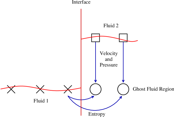
Figure 1: Illustrating the Ghost Fluid boundary condition in one dimension. The boundary condition is to be applied to fluid 1. This is done by creating an artificial “ghost” fluid in the region covered by fluid 2. This ghost fluid obeys the same equations of motion and EOS as fluid 1 and is used to implicitly capture the boundary conditions at the interface. The pressure and (normal) velocity are copied from fluid 2. The entropy (and, in higher dimensions, the tangential velocity) are extrapolated from fluid 1. The same procedure is applied to fluid 2.

III Implementation

III.1 Formulation

III.1.1 Hydrodynamics - flat space

In order to best compare to standard relativistic hydrodynamics simulations we use the conserved formulation of Banyuls et al. (1997). In $1+1$ Minkowski spacetime using Cartesian coordinates and the test-fluid approximation this is written as

$$\partial_{t}{\bf q}+\partial_{x}{\bf f}({\bf q})={\bf 0},$$ (6)

where the conserved variables ${\bf q}$ and fluxes ${\bf f}$ are given in terms of the primitive variables introduced in section II by

$${\bf q} =\left(D,S_{x},\tau\right)^{T}=\left(\rho_{0}W,\rho_{0}hW^{2}v_{x},\rho_{0}hW^{2}-p-\rho_{0}W\right)^{T},$$ (7a)

$${\bf f} =\left(Dv^{x},S_{x}v^{x}+p,\left(\tau+p\right)v^{x}\right)^{T},$$ (7b)

where we have introduced the 3-velocity

$$v^{i}=\frac{1}{\alpha}\left(\frac{u^{i}}{u^{t}}+\beta^{i}\right)=\frac{u^{i}}{u^{t}},$$ (8)

where the shift $\beta^{i}$ and lapse $\alpha$ resulting from the $3+1$ split take the trivial values in this case. We have also introduced the Lorentz factor

$$W=\left(1-v_{i}v^{i}\right)^{-1/2}.$$ (9)

To close the system an equation of state is required. In this paper we use the simple $\gamma$-law equation of state

$$p(\rho_{0},\epsilon)=(\gamma-1)\rho_{0}\epsilon,$$ (10)

where $\gamma$ is the ratio of specific heats. Different regions of spacetime may have different equations of state which is modelled simply by providing different values of $\gamma$.

The level set equation (4) becomes

$$\partial_{t}\phi+v^{x}\partial_{x}\phi=0.$$ (11)

This equation is not in conservation law form. Whilst it can be written in conservation law form this would have no advantage, as it is only the zeros of the level set function that have meaning. The non-conservative form of equation (11) is evolved directly.

III.1.2 Hydrodynamics - spherical symmetry

In $1+1$ spherical symmetry we follow e.g. Romero et al. (1996); Neilsen (1999); Noble (2003) in using polar-areal coordinates. The line element is written

$$\text{d}s^{2}=-\alpha^{2}(t,r)\text{d}t^{2}+a^{2}(t,r)\text{d}r^{2}+r^{2}\left(\text{d}\theta^{2}+\sin^{2}\theta\,\text{d}\phi^{2}\right).$$ (12)

The 3-velocity becomes

$$v^{r}=\frac{u^{r}}{\alpha u^{t}}.$$ (13)

The conservation law form is written

$$\partial_{t}\left(a{\bf q}\right)+\frac{1}{r^{2}}\partial_{r}\left(\alpha ar^{2}{\bf f}({\bf q})\right)={\bf s}({\bf q}),$$ (14)

where the variables, fluxes and sources are

$${\bf q} =\left(D,S_{r},\tau\right)^{T}=\left(\rho_{0}W,\rho_{0}hW^{2}v_{r},\rho_{0}hW^{2}-p-\rho_{0}W\right)^{T},$$ (15a)

$${\bf f} =\left(Dv^{r},S_{r}v^{r}+p,\left(\tau+p\right)v^{r}\right)^{T},$$ (15b)

$${\bf s} =\alpha a\left(0,-\frac{a^{2}m}{r^{2}}\left(S_{r}v^{r}+\tau+p+D\right)+\frac{2p}{r},-\frac{m}{r^{2}}S_{r}\right)^{T},$$ (15c)

where the spacetime quantity $m=\frac{r}{2}\left(1-a^{-2}\right)$ is the mass aspect function. The spacetime quantities satisfy the equations

$$\partial_{t}a =-4\pi r\alpha aS_{r},$$ (16a)

$$\partial_{r}a =a^{3}\left[4\pi r\left(\tau+D\right)-\frac{m}{r^{2}}\right],$$ (16b)

$$\partial_{r}\log(\alpha) =a^{2}\left[4\pi r\left(S_{r}v^{r}+p\right)+\frac{m}{r^{2}}\right].$$ (16c)

We will evolve $a$ using equation (16a) and solve for the lapse using the slicing condition (16c), whilst the error in the Hamiltonian constraint (16b) will be used to check the accuracy of the simulations.

To reduce problems near the coordinate singularity at the origin the equations are rewritten as

$$\partial_{t}\left(a{\bf q}\right)+\frac{1}{3}\partial_{r^{3}}\left(\alpha ar^{2}{\bf f}^{(1)}({\bf q})\right)+\partial_{r}\left(\alpha a{\bf f}^{(2)}({\bf q})\right)=\bar{\bf s}({\bf q}),$$ (17)

where the revised fluxes and sources are

$${\bf f}^{(1)} =\left(Dv^{r},S_{r}v^{r},\left(\tau+p\right)v^{r}\right)^{T},$$ (18a)

$${\bf f}^{(2)} =\left(0,p,0\right)^{T},$$ (18b)

$$\bar{\bf s} =\alpha a\left(0,-\frac{a^{2}m}{r^{2}}\left(S_{r}v^{r}+\tau+p+D\right),-\frac{m}{r^{2}}S_{r}\right)^{T}.$$ (18c)

The level set equation (4) becomes

$$\partial_{t}\phi+\alpha v^{r}\partial_{r}\phi=0.$$ (19)

As in flat space, this non-conservative form is evolved directly.

III.2 Numerical methods

To evolve in time the method of lines is used with a second order Runge-Kutta algorithm.

III.2.1 Hydrodynamics

To illustrate the utility of the approach and the Ghost Fluid boundary condition we have used standard High Resolution Shock Capturing (HRSC) methods to solve the hydrodynamics equations (6) and (17). The domain is split into cells, and the conserved variables updated using

$$\frac{\text{d}}{\text{d}t}\hat{\bf q}_{i}=\frac{1}{\Delta x_{i}}\left[\hat{\bf f}_{i-1/2}-\hat{\bf f}_{i+1/2}\right].$$ (20)

Following e.g. Hawke et al. (2005) we concentrate on Reconstruction-Evolution methods, where the variables are reconstructed to cell boundaries and a Riemann problem (approximately) solved to find the inter-cell flux $\hat{\bf f}_{i\pm 1/2}$. For reconstruction we use slope-limited TVD methods with van Leer’s monotized-centred (MC) limiter (van Leer (1973)), or the PPM method (Colella and Woodward (1984); Martí and Müller (1996)). For simplicity we use the HLLE flux formula Einfeldt (1988) in what follows, although we have seen no qualitative difference when the Marquina flux formula Donat and Marquina (1996) is used instead.

III.2.2 Level set

The evolution of the level set (equation (11) or (19)) cannot use the same numerical methods as the equation is not in conservation law form. Instead we shall follow the methods outlined in Osher and Fedkiw (2003), evolving the level set equation as a Hamilton-Jacobi equation. General high-order methods for evolving Hamilton-Jacobi equations can be found, for example, in Shu (1999).

The general method for Hamilton-Jacobi equations of the form

$$\partial_{t}\phi+H(\partial_{x}\phi)=0$$ (21)

that works even when the level set $\phi$ is not differentiable is to solve

$$\frac{\text{d}}{\text{d}t}\phi_{i}+\hat{H}\left(D^{x}_{+}\phi_{i},D^{x}_{-}\phi_{i}\right)=0,$$ (22)

where $\phi_{i}$ is the numerical value of $\phi$ at gridpoint $x_{i}$, $\hat{H}$ the numerical Hamiltonian, assumed Lipschitz continuous, and $D^{x}_{\pm}$ appropriate winded approximations of $\partial_{x}\phi$.

It is simple to use ENO or WENO methods to find the appropriate $D^{x}_{\pm}$ operators (explicit expressions for low order are given by Osher and Fedkiw (2003)). In the $1+1$ examples studied here it has been sufficient to use first order accurate upwind differencing. We would not expect this to be sufficient in more complex examples or in higher dimensions.

We have also used the simple Lax-Friedrichs approximation to the Hamiltonian,

$$\hat{H}(u_{+},u_{-})=H\left(\frac{u_{+}+u_{-}}{2}\right)-\hat{\alpha}\left(\frac{u_{+}-u_{-}}{2}\right),$$ (23)

where $\hat{\alpha}$ is the maximum absolute value of $H$ over the entire domain. In higher dimensions it may be costly to compute $\hat{\alpha}$ over the whole domain, so a local Lax-Friedrichs method (where the maximum value of $\hat{\alpha}$ over the numerical stencil is used) can be used instead.

III.2.3 Ghost Fluid boundary condition

Figure 1 has already been given to illustrate how the Ghost Fluid boundary condition is implemented. To be explicit, we consider a numerical grid $\left\{x_{i}\right\}$ on which the level set $\phi_{i}$ changes sign between points $I,I+1$. We apply the Ghost Fluid boundary condition to fluid 1, which covers the domain to the left of the interface, using where necessary information from fluid 2, which covers the domain to the right of the interface. We will apply the boundary condition to at least $p+1$ “ghost” points extending from $x_{I+1}$ to $x_{I+p+1}$, where $p$ is the stencil size of the numerical method. The reason for the use of $p+1$ ghost points is that at least one additional point is needed if the interface should move one point to the right during the evolution step.

The normal component of the velocity and the pressure of fluid 1, $v^{(1)}$ and $p^{(1)}$ respectively, are copied from fluid 2. The entropy is extrapolated from fluid 1. In the Ghost Fluid method zero order extrapolation normal to the interface is used. In the $1+1$ dimensional cases here, the extrapolation is a simple copy. Explicitly we have

$$v^{(1)}_{j} =v^{(2)}_{j}, j =I+1,\dots,I+p+1,$$ (24a)

$$p^{(1)}_{j} =p^{(2)}_{j}, j =I+1,\dots,I+p+1,$$ (24b)

$$s^{(1)}_{j} =s^{(1)}_{I}, j =I+1,\dots,I+p+1.$$ (24c)

All other hydrodynamical quantities are found from the pressure, entropy, and the equation of state.

III.2.4 The evolution step

In simple cases such as flat space or where free evolution of spacetime quantities is used, the evolution step is now simply a matter of updating both the fluid and level set. However, should key spacetime quantities (such as $a$ for the case given in section III.1.2) be updated using non-local equations (for example, the constraint (16b) could be used to give $a$) then the order of the update becomes important. For this reason we ensure that we update the level set using the methods of section III.2.2 before the hydrodynamical quantities can be updated using the methods of section III.2.1.

We represent a complete evolution step, assuming a first order time-stepping algorithm, as:

1. Given data $\left\{\hat{\bf q}^{n}_{i}\right\}$ for the hydrodynamical variables and $\left\{\phi^{n}_{i}\right\}$ for the level set and timestep $n$.

2. Find interface locations $\left\{x_{j}^{n}:\phi=0\right\},j=0,\dots,N^{n}$, where $N^{n}-1$ is the number of interfaces at time $t^{n}$. For simplicity we denote the boundaries of the computational domain by $x_{0}^{n}$ and $x_{N^{n}}^{n}$ respectively.

3. If there is only one genuine interface approximate the velocity $v$ there.

4. Compute the updated level set $\phi^{n+1}$, either using the interface velocity approximated in the previous step, or using the velocity of the fluid at each point.

5. Compute the new interface locations $\left\{x_{j}^{n+1}:\phi=0\right\},j=0,\dots,N^{n+1}$.

6. For each domain $\Omega_{j}^{n}=[x^{n}_{j},x^{n}_{j+1}],j=0,\dots,N^{n}-1$:

   1. Check the domain still exists at the next time step, $\Omega_{j}^{n+1}\neq\left\{\emptyset\right\}$. If it is, go to the next domain.

   2. Apply the Ghost Fluid boundary condition to both boundaries, extending the domain by a sufficient number of points, as given in section III.2.3.

   3. Compute the inter-cell fluxes on this extended domain.

   4. Restrict the updated variables to the domain $\Omega_{j}^{n+1}=[x^{n+1}_{j},x^{n+1}_{j+1}]$.

   5. Compute primitive variables and apply physical or symmetry boundary conditions as required.

Extending this to higher order in time is trivial with method of lines type methods.

IV Tests

The tests used here are intended to see whether the Ghost Fluid method works in relativistic situations as it does in Newtonian theory. This will indicate whether this is a viable approach for numerical simulations of more complex models of NS interactions such as mergers. The simplest test is a check that the method would keep a single non-interacting material interface stable. This is provided in appendix A as part of an illustration of why capturing an interface is not straightforward numerically, as discussed in section II.2.1.

We start by looking at the interaction between strong nonlinear features and interfaces in flat space, using the model of section III.1.1. These ensure that no spurious oscillations are introduced and see how accurately the method captures transient and long-lived smooth features. We then move on to full GR tests, where we can assess the accuracy and effectiveness with simple spherically symmetric NS models, both stable and nonlinearly perturbed.

IV.1 Flat space tests

IV.1.1 Shock-interface interaction

Two tests are considered. In both the domain is $x\in[0,1]$. In the first a stable material interface is set up in the middle of the domain across which the equation of state changes due to a change in $\gamma$. A mild shock is injected from the left edge of the domain. By time $t=1$ the shock has interacted with the interface, being reflected and transmitted. In this test, which is a modified relativistic analogue of test B of Fedkiw et al. (1999), the precise initial data is

$$\left\{\begin{array}[]{clclclclc}\rho_{0}=&1.3346,&v=&0.1837,&p=&1.5,&\gamma=&1.4&x<0.05\\ \rho_{0}=&1,&v=&0,&p=&1,&\gamma=&1.4&0.05\leq x<0.5\\ \rho_{0}=&1,&v=&0,&p=&1,&\gamma=&1.67&x\geq 0.5.\end{array}\right.$$ (25)

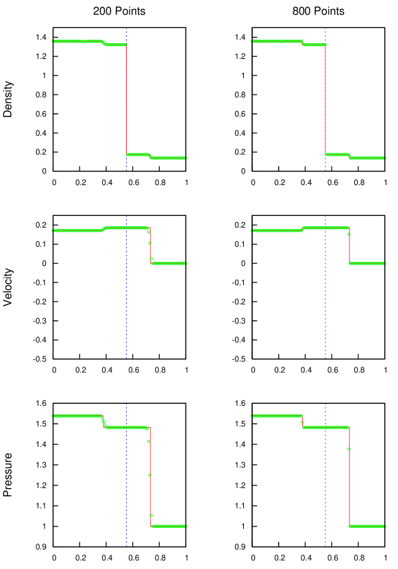
Figure 2: Results from an isolated shock hitting a contact discontinuity, (‘test B’ from Fedkiw et al. (1999)). The transmitted shock is very obvious in the velocity and pressure profiles, and convergence of the solution at this point can be seen. The reflected rarefaction wave is considerably smaller, but can still be seen. The contact discontinuity, shown by the dashed line, is captured correctly. TVD reconstruction using the MC limiter is used, and only 100 points are shown in each plot.

Results from this test are shown in figure 2. For simplicity we use TVD reconstruction with the HLLE Riemann solver. The transmitted shock and reflected rarefaction are clearly seen, with the results converging towards the exact solution. The material interface has propagated to the right due to the interaction, and this is also captured accurately. No spurious oscillations have been generated either at the shock or at the material interface.

A considerably more difficult test that does not have an exact solution was suggested by Wang et al. (2004). This has a “slab” of helium/air mixture initially at rest in air. A moderate shock then strikes the slab, with the resulting shocks and rarefaction interacting multiple times. This is a 1d restriction of the shock-bubble interaction used in the original Ghost Fluid paper Fedkiw et al. (1999). The relativistic analogue used here has initial data

$$\left\{\begin{array}[]{clclclclc}\rho_{0}=&1.37795,&v=&0.17933,&p=&1.57,&\gamma=&1.4&x<0.25\\ \rho_{0}=&1,&v=&0,&p=&1,&\gamma=&1.4&0.25\leq x<0.45\\ \rho_{0}=&0.138,&v=&0,&p=&1,&\gamma=&1.67&0.45\leq x<0.55\\ \rho_{0}=&1,&v=&0,&p=&1,&\gamma=&1.4&x\geq 0.55.\end{array}\right.$$ (26)

The test is run to $t=0.8$.

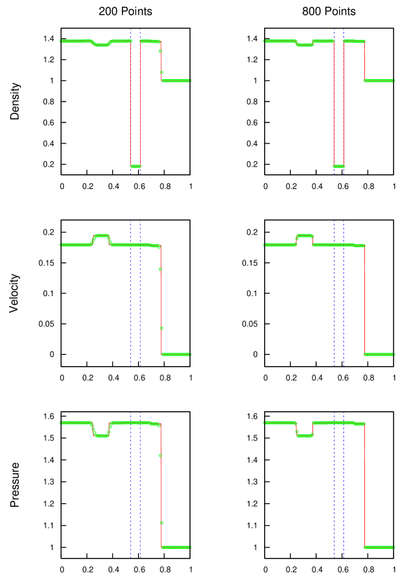
Figure 3: The results for an isolated shock wave hitting a low density slab of material. Multiple reflected and transmitted waves can be seen, as expected. The movement and compression of the low density slab is also apparent. Velocity and pressure once again remain continuous at the interface as desired. TVD reconstruction using the MC limiter is used, and only 100 points are shown in each plot.

Results for this more complex interaction are shown in figure 3. TVD reconstruction using the MC limiter is used. The strong interacting features are captured, with the interfaces moving independently in reaction to the shocks. No oscillations occur, and the result converges with resolution.

IV.1.2 Perturbed shock

A more complex example is that of a shock perturbed by a strong, smooth feature. This test, suggested by Dolezal and Wong (1995) and used e.g. by Del Zanna and Bucciantini (2002), does not have an exact solution, so is compared to a reference solution computed with 12800 points. We modify this test to include an interface, using the initial data

$$\left\{\begin{array}[]{clclclclc}\rho_{0}=&5,&v=&0,&p=&50,&\gamma=&1.4&x<0.5\\ \rho_{0}=&2+0.3\sin(50x),&v=&0,&p=&5,&\gamma=&1.67&x\geq 0.5\end{array}\right..$$ (27)

Again the domain is $x\in[0,1]$ and the test is run to time $t=0.35$.

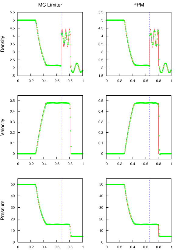
Figure 4: Results for a test with a shock tube test with a sine wave density profile for 200 points. The higher accuracy when using PPM is evident in the post shock density profile, with the sine wave being captured more accurately. The solid line shows a reference solution computed using 12800 points.

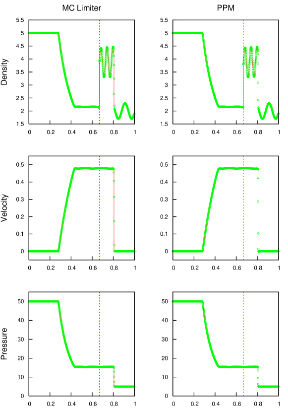
Figure 5: Results for a test with a shock tube test with a sine wave density profile for 800 points. In addition to greater accuracy for the maxima and minima of the sine wave, similar improvements in accuracy at the shock wave are visible for this test.

Results for this test are shown in figures 4 and 5. It is clear that the results are converging to the correct solution irrespective of the numerical method used. No spurious oscillations are introduced. However, it appears that there is a slight discrepancy at the material interface. In particular, the edges of the smooth feature do not appear quite correct. We investigate this with another test.

IV.1.3 Moving sine wave

A final flat space test is adapted from a Newtonian test suggested by Lombard and Donat (2005). A sine wave is advected in a surrounding flow. The material interfaces should be stable, and so the evolution should be trivial. The initial data used here is

$$\left\{\begin{array}[]{clclclclc}\rho_{0}=&1,&v=&0.5,&p=&1,&\gamma=&1.4&x<0.16\\ \rho_{0}=&1+0.3\sin(50(x-0.16)),&v=&0.5,&p=&1,&\gamma=&1.67&0.16\leq x<0.537\\ \rho_{0}=&1,&v=&0.5,&p=&1,&\gamma=&1.4&x\geq 0.537\end{array}\right..$$ (28)

Again the domain is $x\in[0,1]$ and the test is run to time $t=0.4$.

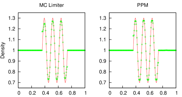
Figure 6: An advected sine wave, evolved with a resolution of 200 points. Since the initial density profile is simply advected with the fluid velocity, an exact solution exists for this test. The differences between the two reconstruction methods are evident, with the PPM test has more accurately capturing the sine wave.

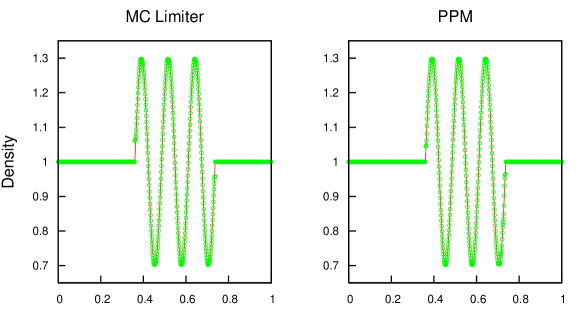
Figure 7: An advected sine wave, evolved with a resolution of 800 points. The sine wave is now captured well with both techniques, though at the interface between the fluids there is still some error. Comparing to figure 6 shows the (slow) convergence of this error.

Results for this test are shown in figures 6 and 7. The majority of the features are well captured and no spurious oscillations are introduced at the material interfaces. It is clear, however, that the accuracy suffers near the interfaces due to the strong gradients there, and the overly simple Ghost Fluid boundary condition. This converges with resolution. We will see in the next section that in simple GR simulations modelling neutron stars this is not a major concern.

IV.2 GR tests

In this section we look at tests in nonlinear general relativity, focusing on tests relevant for neutron stars. We use the system of equations outlined in section III.1.2. All of the tests look at static or nonlinearly perturbed TOV stars in spherical symmetry. The initial data is always constructed with a polytropic EOS

$$p=K\rho_{0}^{\gamma}$$ (29)

where $K$ is the polytropic constant, and evolved with the ideal fluid EOS of equation (10), where $\gamma$ may vary in space.

IV.2.1 Static stars

As a reference solution we construct and evolve a standard static single component star. The initial data is determined by the initial central density $\rho_{0}(t=0,r=0)$ denoted $\rho_{c}$, and the EOS. Here we use the values

$$\rho_{c}=1.28\times 10^{-3},\qquad\gamma=2,\qquad K=100.$$ (30)

We then evolve this using the TVD method as described in section III.2.

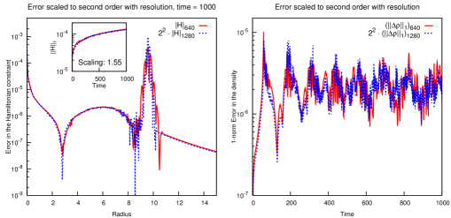
Figure 8: A single component TOV star is evolved as a reference case. The error in the Hamiltonian constraint is shown as a function of space at late time in the left panel, with the time-dependent behaviour of the 1-norm shown in the inset. Simulations with 640 and 1280 points are shown, with the behaviour in space scaled for second order convergence. The behaviour of the norm is scaled for convergence order 1.55. Second order convergence is observed nearly everywhere. The surface, located near $r\sim 10$, is the clear location where the order of convergence is reduced, as expected. This leads to the reduced order of convergence in the 1-norm. In the right panel the 1-norm of the density errors is shown, scaled for second order convergence. Here the impact of the surface errors is not so pronounced, so second order convergence in the norm is approached.

The errors in the evolution are shown in figure 8. Second order convergence is seen over the majority of space at late time. However, near the surface of the star convergence is lost, both due to the “clipping” inherent in HRSC methods, and due to the atmosphere algorithm used here. This is the dominant factor in reducing the order of convergence of the norms.

As a first test of the accuracy of the Ghost Fluid algorithm in GR we then introduce a “trivial” interface into the TOV star at coordinate location $r=3.015$. On either side of this interface the EOS is the same as that given in equation (30). We then evolve, imposing the Ghost Fluid boundary condition at the interface. It should be noted that in this simulation, although the level set is evolved the interface inferred from the zero of the level set remains within the same grid cell at all times.

Figure 9: A single component TOV star with an interface artificially introduced at $r=3.015$ is evolved. These results should be compared with the reference solution in figure 8. The accuracy and convergence properties are nearly identical to the reference solution.

As can be seen from figure 9, by comparing to the reference solution of figure 8, the Ghost Fluid method makes virtually no difference to the accuracy of the results. The convergence properties are nearly identical, and the effect of the interface is very difficult to detect in the errors.

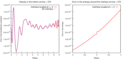
Figure 10: A closer look at the evolution of the single component TOV star with the artificial interface at $r\simeq 3$. Only the simulation using 1280 points is shown. In the left panel the radial 3-velocity component is shown. As expected, the velocity is continuous across the interface. The difference between this evolution and the reference solution are due to interactions between the errors introduced by the surface and the interface, and are strongest near the surface. In the right panel the change in the entropy between the initial data and $t\simeq 270$ is shown. As the entropy is extrapolated across the interface this shows the jump induced by the Ghost Fluid boundary condition; however, the size of this error is negligible.

To look at the effect of the Ghost Fluid boundary condition in more detail, in figure 10 we show the difference in the radial 3-velocity component between the reference evolution without the interface and the evolution containing the interface. The effect of the interface is not directly obvious in the plot. The velocity should be continuous at the interface, and clearly is. The differences between the two evolutions appear near the surface of the star, which is where the velocity is largest. This indicates that the differences are due to minor reflections from the interface which are clearly at a very low level. In addition we look at the change in the entropy during the evolution. The entropy is extrapolated by the Ghost Fluid algorithm, so should show the effect of the boundary condition. The initial entropy is ${\cal O}(1)$, so whilst the effect of the boundary condition is clear in inducing a small jump at the interface, the magnitude of the effect at $\sim 10^{-7}$ is clearly negligible.

We then move on to look at static stars containing a genuine interface between two different components. We have studied a number of different configurations, with the qualitative behaviour being similar in all cases. As an illustration we use the initial data

$$\left\{\begin{array}[]{clclclc}\rho_{c}=&6\times 10^{-4},&\gamma=&2,&K=&100,&r<3.015\\ &&\gamma=&\frac{5}{3},&K=&11.17,&r\geq 3.015\end{array}\right..$$ (31)

This ensures the TOV is stable, and that pressure and its first derivative are continuous at the interface. This initial data is illustrated in figure 11.

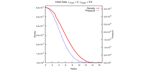
Figure 11: The initial data used for the evolution of a two component star. The outer fluid uses a softer EOS than the reference solution, leading to a larger radius. The interface at $r\simeq 3$ is clearly seen from the density jump.

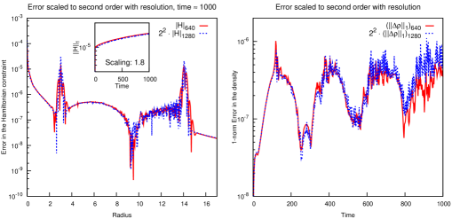
Figure 12: Errors introduced in evolving a two component star. This should be compared to the reference solution in figure 8 and the artificial interface solution in figure 9. The interface at $r\simeq 3$ now has a visible effect in the errors, but these are still manageable and converge. Note that at these resolutions the convergence of the norm of the constraints is actually better than in the reference solution, as the errors in the interior (which converge at second order) are larger due to the non-trivial interface, whilst those near the surface (which converge at less than second order) are smaller due to the softer EOS. The errors in the density show good convergence until late times when the errors near the surface become sufficiently large.

The result of the evolution is shown in figure 12. In this case we do see an effect in the Hamiltonian constraint from the interface at $r=3.015$. This leads to larger errors within the star (at fixed resolution). However, these errors appear to converge at second order (except for the points directly next to the interface). This means that, for these resolutions, the convergence of the constraint error is actually better than for the reference solution shown in figure 8. This is because the error at the surface, which does not converge at second order due to the atmosphere algorithm and the inherent properties of HRSC methods, contributes less (relatively) to the total error. In contrast, the errors in the density are (relatively) larger at the surface as we are using a lower central density and a softer EOS for the outer fluid. Hence at late times as the surface errors increase the effects are seen in the errors of the density, which drifts away from perfect second order convergence.

IV.2.2 Perturbed star

The tests in section IV.2.1 show that there is no problem in extending the level set method augmented with the Ghost Fluid boundary condition to GR when studying simple solutions. However, we really require that these methods will work in strongly nonlinear situations which will include interface motion and shock formation and interaction. In order to look at this in a 1+1 context we take a two component TOV star and give a strong nonlinear perturbation designed both to move the interface and to produce shocks propagating within the fluid. Due to the limitations of our atmosphere algorithm the results will not be trustworthy when the shocks start to reach the surface of the star, so we keep the evolutions relatively short. However, these evolutions are sufficient to validate the approach that we use here.

The initial data used is based on a two component TOV star with parameters

$$\left\{\begin{array}[]{clclclc}\rho_{c}=&1.28\times 10^{-3},&\gamma=&2,&K=&100,&r<3.015\\ &&\gamma=&1.9,&K=&51.57,&r\geq 3.015\end{array}\right..$$ (32)

The interior is then perturbed using

$$\rho_{0}=\left(\rho_{0}\right)_{\text{TOV}}\left(1+h(r)\right),\quad p=p_{\text{TOV}}\left(1+h(r)\right),$$ (33)

where

$$h(r)=\begin{cases}\frac{1}{20}\left(1-\tanh\left[50(r-2)\right]\right)&r<2.5,\\ 0&r\geq 2.5.\end{cases}$$ (34)

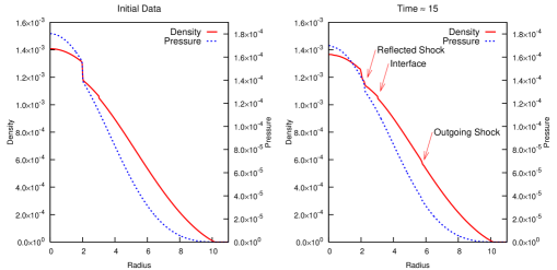
Figure 13: The left panel shows the initial data for the nonlinearly perturbed two component star. The interior perturbation near $r\simeq 2$ is not quite a shock but will trigger an outgoing wave that steepens into a shock before passing through the interface at $r\simeq 3$. It will also produce a strong ingoing wave that will reflect from the origin, producing another shock. The right panel shows the evolved at a time when the initial outgoing shock has passed through the interface but before the reflected shock has had time to reach it.

This is illustrated in the left panel of figure 13. The strong perturbation leads to a very steep feature near $r\simeq 2$ that will form a shock and move the interface. As seen in the right panel of figure 13, there is an additional shock formed by the “ingoing” piece of the initial perturbation reflecting from the origin; at the time of this plot it has not reached the interface.

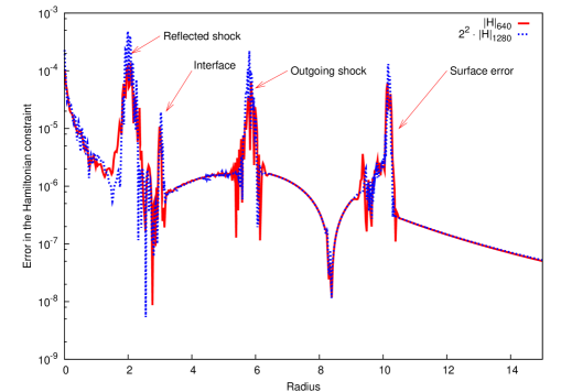
Figure 14: Constraint errors in the evolution of the nonlinearly perturbed star. The curves are scaled for second order convergence, which is seen away from the surface and the shocks.

The constraint errors in the evolution of the nonlinearly perturbed star are shown in figure 14. As expected we now see a large number of features indicated on the plot. As in the reference solution in figure 8 we see the error from the surface, which is sizeable and does not converge cleanly at second order. As in the static two component test in figure 11 we see an error at the interface, which in this case is relatively small and converges except at a few points directly neighbouring the interface. Finally we see strong features at the two shocks where, due to the nature of HRSC methods, the order of accuracy is degraded to first order.

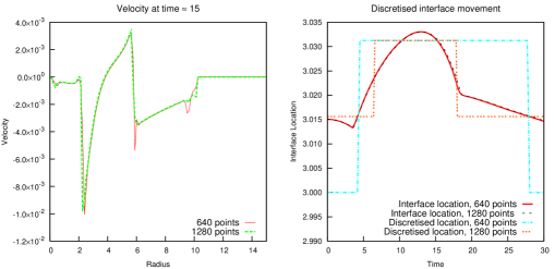
Figure 15: The left panel shows the radial component of the 3-velocity for the nonlinearly perturbed star, indicating the locations of the shocks. By this point the interface, initially at $r=3.015$, has moved outwards and has started to move back in again. As expected the velocity is smooth at the interface and no spurious oscillations have been generated by the interaction with the outgoing shock. The right panel indicates the interface location as a function of time, showing its coordinate location as inferred from the level set, and the computational coordinate of the centre of the cell within which the interface is found. We see that even with this strong perturbation the motion is small but similar for all resolutions.

Figure 15 shows the motion of the interface and also shows that no spurious oscillations occur due to the interaction between the outgoing shock and the interface. The left panel shows the velocity at a time when the outgoing shock has passed through the interface located at $r\simeq 3$. The velocity is continuous with no spurious oscillations, despite the interaction with the shock. The right panel shows the motion of the interface. Initially it falls in, due to the additional matter in the interior. It then interacts with the shock, being pushed outwards and jumping between cells, before starting to fall back again, with the additional interaction with the reflected shock at $t\simeq 18$ being insufficient to stop its inward motion.

V Conclusions

In this paper we have considered models of relativistic matter containing sharp interfaces and their particular importance and implementation for numerical simulations. We expect that simulations of realistic models of neutron stars, as required for gravitational wave template calculations, will contain features that will be too sharp to be resolved as a smooth feature using reasonable numerical resolution. It follows that models incorporating sharp interfaces and techniques for evolving them cleanly will be required.

The use of level set techniques to capture and evolve the interfaces that might form and disappear through mergers is already well known in numerical relativity, particularly in the context of event horizon finders. Their use here is natural and simple, and should allow the techniques investigated here to easily be extended to more spatial dimensions.

However, the description of the interface location is not sufficient. We must impose a boundary condition at the interface, which will complete the description of the continuum model. The Ghost Fluid boundary condition used here has the advantage of simplicity, which makes it ideal for a proof-of-principle test such as this. However, it is questionable if this condition is sufficient for all situations, and more advanced techniques may be required with more complex EOSs than those considered here.

The results of section IV illustrate the advantages of the combined level set and Ghost Fluid method. It is simple, and for strong shocks or smooth flow interacting with interfaces it gives good results. We have shown that it directly extends to GR, and that for mildly perturbed neutron star tests the results are stable, convergent, and as accurate as the numerical method employed. However, when there is a long-lasting, strong feature that interacts with the interface, the test shown in section IV.1.3 illustrates the limitations of the technique. This may indicate the need for better boundary conditions at the interface before high accuracy simulations for gravitational wave extraction can be attempted for complex neutron star models.

Acknowledgements:

IH was supported by the STFC rolling grant PP/E001025/1 and Nuffield Foundation grant NAL/32622. SM was supported by an EPSRC studentship.

Appendix A Colour functions

At first glance it would appear that the simple tests shown in this paper are solved with an excessively complex numerical method. From the simplest point of view, our system of equations describing relativistic hydrodynamics has simply been augmented with an equation of motion for the EOS parameter $\gamma$. This can be described by a “colour function” and advected using standard HRSC methods if written in the form

$$\partial_{t}\left(\rho_{0}\gamma\right)+\partial_{i}\left(\rho_{0}\gamma v^{i}\right)=0.$$ (35)

In fact any parameter $\kappa$ required by the EOS can be advected using an equation of this form.

However, it is well known in the CFD literature that this naïve approach fails for the simplest interfaces.

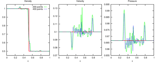
Figure 16: A stable contact discontinuity, initially at $x=0.5$, with the fluid to the left having $\gamma=5/3$ and the fluid to the right having $\gamma=4/3$ is advected to the right with speed $0.1$. The initial data is set such that the interface should propagate unchanged. The plot shows this initial data evolved using two resolutions and standard HRSC methods to time $t=0.2$ using the colour function approach, with the exact solution given by the solid line. Spurious oscillations are introduced at the interface. These oscillations do not converge with resolution, indicating a failure of the approach.

Figure 16 shows this approach failing for a stable material interface. The interface is set at $x=0.5$, with initial data

$$\left(\rho_{0},v,p,\gamma\right)=\begin{cases}\left(1,0.1,\tfrac{2}{3},\tfrac{5}{3}\right)&x<0.5,\\ \left(\tfrac{1}{2},0.1,\tfrac{2}{3},\tfrac{4}{3}\right)&x\geq 0.5,\end{cases}$$ (36)

leading to a stable interface propagating to the right. The standard conservation law form, as in section III.1.1, augmented with the colour function equation (35), is evolved using the simple TVD HRSC method used in the rest of the paper. This is considerably simpler than the level set method, but as can be seen from the figure fails utterly to deal with this simple interface. Spurious oscillations are introduced. These oscillations are sizeable and do not converge with resolution. Clearly there is a failure of the approach, which is due to the formulation of the problem.

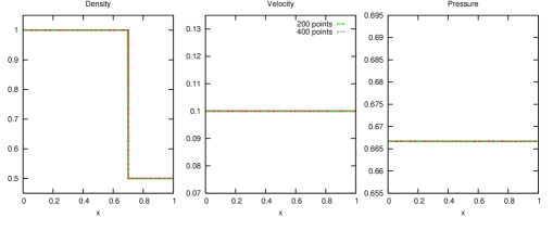
Figure 17: The stable contact discontinuity test evolved to time $t=2$ using the level set method with the Ghost Fluid boundary condition. Comparing to figure 16 we see that there are no spurious oscillations and the interface is captured perfectly at all resolutions.

The level set method combined with the Ghost Fluid boundary condition deals with this situation with no problem whatsoever, as illustrated in figure 17.

The reasons for the failure of the colour function approach have been studied in detail by a number of authors. As explained by Abgrall and Karni (2001) the key is that the inherent “smearing” of the HRSC scheme will effectively “mix” the fluids either side of the interface in a narrow region. The detailed way that the mixing occurs will depend on the resolution and the numerical method, but it will always occur. However, without imposing further conditions it is clear that this mixing will not be thermodynamically consistent. That is, the numerical mixing will lead to spurious generation of entropy at the interface, creating the oscillations observed. Whilst it is possible to construct numerical methods that are thermodynamically consistent (e.g. Wang et al. (2004); for example, for the EOS used here evolving the EOS parameter $\kappa=1/(\gamma-1)$ is consistent, as shown by Abgrall and Karni (2001)) this may not always be straightforward, and the problem of the length over which the interface is smeared, as described in the introduction, remains.

References

- Font (2008) J. A. Font, Living Reviews in Relativity 11 (2008), URL http://www.livingreviews.org/lrr-2008-7.
- Abbott et al. (2009) B. P. Abbott et al., Reports on Progress in Physics 72, 076901 (25pp) (2009), URL http://stacks.iop.org/0034-4885/72/076901.
- Acernese et al. (2006) F. Acernese et al., Class. Quantum Grav. 23, S635 (2006).
- Andersson et al. (2005) N. Andersson, G. L. Comer, and K. Glampedakis, Nucl. Phys. A763, 212 (2005), eprint astro-ph/0411748.
- Harten (1978) A. Harten, Mathematics of Computation 32, 363 (1978), URL http://www.jstor.org/stable/2006149.
- Barnes et al. (2004) A. P. Barnes, P. G. Lefloch, B. G. Schmidt, and J. M. Stewart, Class. Quant. Grav. 21, 5043 (2004).
- Thornburg (2007) J. Thornburg, Living Reviews in Relativity 10 (2007), URL http://www.livingreviews.org/lrr-2007-3.
- Diener (2003) P. Diener, Class. Quant. Grav. 20, 4901 (2003), eprint gr-qc/0305039.
- Osher and Fedkiw (2003) S. Osher and R. Fedkiw, Level Set Methods and Dynamic Implicit Surfaces, vol. 153 of Applied Mathematical Sciences (Springer-Verlag, 2003).
- Sethian (1996) J. Sethian, Level Set Methods and Fast Marching Methods (Cambridge University Press, 1996).
- Fedkiw et al. (1999) R. P. Fedkiw, T. Aslam, B. Merriman, and S. Osher, Journal of Computational Physics 152, 457 (1999), ISSN 0021-9991, URL http://www.sciencedirect.com/science/article/B6WHY-45GMW83-31%/2/78188ca59df6a26d48c72b85a6dfcf4e.
- Liu et al. (2003) T. G. Liu, B. C. Khoo, and K. S. Yeo, Journal of Computational Physics 190, 651 (2003), ISSN 0021-9991, URL http://www.sciencedirect.com/science/article/B6WHY-49324BB-8/%2/09c039d91ac49e11ff1dba4f5d07e88a.
- Liu et al. (2005) T. Liu, B. Khoo, and C. Wang, Journal of Computational Physics 204, 193 (2005), ISSN 0021-9991, URL http://www.sciencedirect.com/science/article/B6WHY-4DTKKXN-1/%2/6155ce6fc7f419d370ba0b8c25d8f5c2.
- Banyuls et al. (1997) F. Banyuls, J. A. Font, J. M. Ibanez, J. M. Marti, , and J. A. Miralles, The Astrophysical Journal 476, 221 (1997), URL http://stacks.iop.org/0004-637X/476/221.
- Romero et al. (1996) J. V. Romero, J. M. A. Ibanez, J. M. A. Marti, and J. A. Miralles, ApJ 462, 839 (1996), eprint arXiv:astro-ph/9509121.
- Neilsen (1999) D. W. Neilsen, Ph.D. thesis, The University of Texas at Austin (1999).
- Noble (2003) S. C. Noble, Ph.D. thesis, The University of Texas at Austin (2003), gr-qc/0310116.
- Hawke et al. (2005) I. Hawke, F. Loffler, and A. Nerozzi, Phys. Rev. D71, 104006 (2005), eprint gr-qc/0501054.
- van Leer (1973) B. J. van Leer, Lecture Notes in Physics 18, 163 (1973).
- Colella and Woodward (1984) P. Colella and P. R. Woodward, Journal of Computational Physics 54, 174 (1984), ISSN 0021-9991, URL http://www.sciencedirect.com/science/article/B6WHY-4DD1PHM-SJ%/2/13d69a59afba3d6a5d6bbf1144d860aa.
- Martí and Müller (1996) J. M. Martí and E. Müller, Journal of Computational Physics 123, 1 (1996), ISSN 0021-9991, URL http://www.sciencedirect.com/science/article/B6WHY-45NJMH5-1D%/2/98a5fc5dfa9977cc99ee640aa2217732.
- Einfeldt (1988) B. Einfeldt, SIAM Journal on Numerical Analysis 25, 294 (1988), URL http://link.aip.org/link/?SNA/25/294/1.
- Donat and Marquina (1996) R. Donat and A. Marquina, Journal of Computational Physics 125, 42 (1996), ISSN 0021-9991, URL http://www.sciencedirect.com/science/article/B6WHY-45MGWCH-62%/2/b14ec3c8a1e12309465c5d9866d54dec.
- Shu (1999) C. W. Shu, in High-Order Methods for Computational Physics, edited by T. J. Barth and H. Deconinck (Springer, 1999).
- Wang et al. (2004) S.-P. Wang, M. H. Anderson, J. G. Oakley, M. L. Corradini, and R. Bonazza, Journal of Computational Physics 195, 528 (2004), ISSN 0021-9991, URL http://www.sciencedirect.com/science/article/B6WHY-4B3NM1S-2/%2/96f62d6bfc07ea12490c213d8a1ab263.
- Dolezal and Wong (1995) A. Dolezal and S. S. M. Wong, Journal of Computational Physics 120, 266 (1995), ISSN 0021-9991, URL http://www.sciencedirect.com/science/article/B6WHY-45NJJFW-1D%/2/8df2ef1b62e40d14d6b0e07fcda05dbd.
- Del Zanna and Bucciantini (2002) L. Del Zanna and N. Bucciantini, A&A 390, 1177 (2002).
- Lombard and Donat (2005) B. Lombard and R. Donat, SIAM Journal on Scientific Computing 27, 208 (2005), URL http://link.aip.org/link/?SCE/27/208/1.
- Abgrall and Karni (2001) R. Abgrall and S. Karni, Journal of Computational Physics 169, 594 (2001), ISSN 0021-9991, URL http://www.sciencedirect.com/science/article/B6WHY-45BC2B2-5C%/2/5494ddc77cb5e2f7ab2c23fe25353675.