Infinitesimals without Logic
Abstract
We introduce the ring of Fermat reals, an extension of the real field containing nilpotent infinitesimals. The construction takes inspiration from Smooth Infinitesimal Analysis (SIA), but provides a powerful theory of actual infinitesimals without any need of a background in mathematical logic. In particular, on the contrary with respect to SIA, which admits models only in intuitionistic logic, the theory of Fermat reals is consistent with classical logic. We face the problem to decide if the product of powers of nilpotent infinitesimals is zero or not, the identity principle for polynomials, the definition and properties of the total order relation. The construction is highly constructive, and every Fermat real admits a clear and order preserving geometrical representation. Using nilpotent infinitesimals, every smooth functions becomes a polynomial because in Taylor’s formulas the rest is now zero. Finally, we present several applications to informal classical calculations used in Physics: now all these calculations become rigorous and, at the same time, formally equal to the informal ones. In particular, an interesting rigorous deduction of the wave equation is given, that clarifies how to formalize the approximations tied with Hook’s law using this language of nilpotent infinitesimals.
I Introduction and general problem
Frequently in work by physicists it is possible to find informal calculations like
| (1) |
with explicit use of infinitesimals or such that e.g. . For example Einstein (1926) wrote the formula (using the equality sign and not the approximate equality sign )
| (2) |
justifying it with the words “since is very small”; the formulas (1) are a particular case of the general (2). Dirac (1975) wrote an analogous equality studying the Newtonian approximation in general relativity.
Using this type of infinitesimals we can write an equality, in some infinitesimal neighborhood, between a smooth function and its tangent straight line, or, in other words, a Taylor’s formula without remainder.
There are obviously many possibilities to formalize this kind of intuitive reasonings, obtaining a more or less good dialectic between informal and formal thinking, and indeed there are several theories of actual infinitesimals (from now on, for simplicity, we will say “infinitesimals” instead of “actual infinitesimals” as opposed to “potential infinitesimals”). Starting from these theories we can see that we can distinguish between two type of definitions of infinitesimals: in the first one we have at least a ring containing the real field and infinitesimals are elements such that for every positive standard real . The second type of infinitesimal is defined using some algebraic property of nilpotency, i.e. for some natural number . For some ring these definitions can coincide, but anyway they lead, of course, only to the trivial infinitesimal if .
However these definitions of infinitesimals correspond to theories which are completely different in nature and underlying ideas. Indeed these theories can be seen in a more interesting way to belong to two different classes. In the first one we can put theories that need a certain amount of non trivial results of mathematical logic, whereas in the second one we have attempts to define sufficiently strong theories of infinitesimals without the use of non trivial results of mathematical logic. In the first class we have Non-Standard Analysis (NSA) and Synthetic Differential Geometry (SDG, also called Smooth Infinitesimal Analysis, see e.g. Bell (1998); Kock (1981); Lavendhomme (1996); Moerdijk and Reyes (1991)), in the second one we have, e.g., Weil functors (see Kriegl and Michor (1996)), Levi-Civita fields (see Shamseddine (1999); Berz (1994)), surreal numbers (see Conway (1976); Ehresmann (1951)), geometries over rings containing infinitesimals (see Bertram (2008)). More precisely we can say that to work in NSA and SDG one needs a formal control deeply stronger than the one used in “standard mathematics”. Indeed to use NSA one has to be able to formally write the sentences one needs to use the transfer theorem. Whereas SDG does not admit models in classical logic, but in intuitionistic logic only, and hence we have to be sure that in our proofs there is no use of the law of the excluded middle, or e.g. of the classical part of De Morgan’s law or of some form of the axiom of choice or of the implication of double negation toward affirmation and any other logical principle which is not valid in intuitionistic logic. Physicists, engineers, but also the greatest part of mathematicians are not used to have this strong formal control in their work, and it is for this reason that there are attempts to present both NSA and SDG reducing as much as possible the necessary formal control, even if at some level this is technically impossible (see e.g. Henson (1997), and Benci and Di Nasso (2003, 2005) for NSA; Bell (1998) and Lavendhomme (1996) for SDG, where using an axiomatic approach the authors try to postpone the very difficult construction of an intuitionistic model of a whole set theory using Topos).
On the other hand NSA is essentially the only theory of infinitesimals with a discrete diffusion and a sufficiently great community of working mathematicians and published results in several areas of mathematics and its applications, see e.g. Albeverio et al. (1988). SDG is the only theory of infinitesimals with non trivial, new and published results in differential geometry concerning infinite dimensional spaces like the space of all the diffeomorphisms of a generic (e.g. non compact) smooth manifold. In NSA we have only few results concerning differential geometry. Other theories of infinitesimals have not, at least up to now, the same formal strength of NSA or SDG or the same potentiality to be applied in several different areas of mathematics.
Our main aim, of which the present work represents a first step, is to find a theory of infinitesimals within “standard mathematics” (in the precise sense explained above of a formal control more “standard” and not so strong as the one needed e.g. in NSA or SDG) with results comparable with those of SDG, without forcing the reader to learn a strong formal control of the mathematics he/she is doing. Because it has to be considered inside “standard mathematics”, our theory of infinitesimals must be compatible with classical logic.
Concretely, the idea of the present work is to by-pass the impossibility theorem about the incompatibility of SDG with classical logic that forces SDG to find models within intuitionistic logic.
Another point of view about present theories of infinitesimals is that, in spite of the fact that frequently they are presented using opposed motivations, they lacks the intuitive interpretation of what the powerful formalism permits to do. For some concrete example in this direction, see Giordano (2009). Another aim of the present work is to construct a new theory of infinitesimals preserving always a very good dialectic between formal properties and intuitive interpretation.
More technically we want to show that it is possible to extend the real field adding nilpotent infinitesimals, arriving at an enlarged real line , by means of a very simple construction completely inside “standard mathematics”. Indeed to define the extension we shall use elementary analysis only. To avoid misunderstandings is it important to clarify that the purpose of the present work is not to give an alternative foundation of differential and integral calculus (like NSA), but to obtain a theory of nilpotent infinitesimals as a first step for the foundation of a smooth () differential geometry. For some preliminary results in this direction, see Giordano (2009).
II Motivations for the name “Fermat reals”
It is well known that historically two possible reductionist constructions of the real field starting from the rationals have been made. The first one is Dedekind’s order completion using sections of rationals, the second one is Cauchy’s metric space completion. Of course there are no historical reason to attribute our extension of the real field, to be described below, to Fermat, but there are strong motivations to say that, probably, he would have liked the underlying spirit and some properties of our theory. For example:
-
1.
a formalization of Fermat’s infinitesimal method to derive functions is provable in our theory. We recall that Fermat’s idea was, roughly speaking and not on the basis of an accurate historical analysis which goes beyond the scope of the present work (see e.g. Edwards (1979); Eves (1990)), to suppose first , to construct the incremental ratio
and, after suitable simplifications (sometimes using infinitesimal properties), to take in the final result .
-
2.
Fermat’s method to find the maximum or minimum of a given function at was to take to be extremely small so that the value of was approximately equal to that of . In modern, algebraic language, it can be said that only if , that is if is a first order infinitesimal. Fermat was aware that this is not a “true” equality but some kind of approximation (ibidem). We will follow a similar idea to define introducing a suitable equivalence relation to represent this equality.
-
3.
Fermat has been described by Bell (1937) as “the king of amateurs” of mathematics, and hence we can suppose that in its mathematical work the informal/intuitive part was stronger with respect to the formal one. For this reason we can think that he would have liked our idea to obtain a theory of infinitesimals preserving always the intuitive meaning and without forcing the working mathematician to be too much formal.
For these reason we chose the name “Fermat reals” for our ring (note: without the possessive case, to underline that we are not attributing our construction of to Fermat).
III Definition and algebraic properties of Fermat reals: The basic idea
We start from the idea that a smooth () function is actually equal to its tangent straight line in the first order neighborhood e.g. of the point , that is
| (3) |
where is the subset of which defines the above-mentioned neighborhood of . The equality (3) can be seen as a first-order Taylor’s formula without remainder because intuitively we think that for any (indeed the property defines the first order neighborhood of in ). These almost trivial considerations lead us to understand many things: must necessarily be a ring and not a field because in a field the equation implies ; moreover we will surely have some limitation in the extension of some function from to , e.g. the square root, because using this function with the usual properties, once again the equation implies . On the other hand, we are also led to ask whether (3) uniquely determines the derivative : because, even if it is true that we cannot simplify by , we know that the polynomial coefficients of a Taylor’s formula are unique in classical analysis. In fact we will prove that
| (4) |
that is the slope of the tangent is uniquely determined in case it is an ordinary real number. We will call formulas like (4) derivation formulas.
If we try to construct a model for (4) a natural idea is to think our new numbers in as equivalence classes of usual functions . In this way we may hope both to include the real field using classes generated by constant functions, and that the class generated by could be a first order infinitesimal number. To understand how to define this equivalence relation we have to think at (3) in the following sense:
| (5) |
where the idea is that we are going to define . If we think “sufficiently similar to ”, we can define so that (5) is equivalent to
that is
| (6) |
In this way (5) is very near to the definition of differentiability for at 0.
It is important to note that, because of de L’Hpital’s theorem we have the isomorphism
the left hand side is (isomorphic to) the usual tangent bundle of and thus we obtain nothing new. It is not easy to understand what set of functions we have to choose for , in (6) so as to obtain a non trivial structure. The first idea is to take continuous functions at , instead of more regular ones like -functions, so that e.g. becomes a -th order nilpotent infinitesimal (); indeed for almost all the results presented in this article, continuous functions at work well. However, only in proving the non-trivial property
| (7) |
we can see that it does not suffice to take continuous functions at . To prove (7) the following functions turned out to be very useful:
Definition 1.
If , then we say that is nilpotent iff as , for some . will denote the set of all the nilpotent functions.
E.g. any Hoelder function (for some constant ) is nilpotent. The choice of nilpotent functions instead of more regular ones establish a great difference of our approach with respect to the classical definition of jets (see e.g. Bröcker (1975); Golubitsky and Guillemin (1973)), that (6) may recall.
Another problem necessarily connected with the basic idea (3) is that the use of nilpotent infinitesimals very frequently leads to consider terms like . For this type of products the first problem is to know whether and what is the order of this new infinitesimal, that is for what we have but . We will have a good frame if we will be able to solve these problems starting from the order of each infinitesimal and from the values of the powers . On the other hand almost all the examples of nilpotent infinitesimals are of the form , with , and their sums; these functions have also great properties in the treatment of products of powers. It is for these reasons that we shall focus our attention on the following family of functions in the definition (6) of :
Definition 2.
We say that is a little-oh polynomial, and we write iff
-
1.
-
2.
We can write
for suitable
Hence a little-oh polynomial is a polynomial function with real coefficients, in the real variable , with generic positive powers of , and up to a little-oh function as .
Remark 3.
In the following, writing as we will always mean
In other words, every little-oh function we will consider is continuous as .
Example.
Simple examples of little-oh polynomials are the following:
-
1.
-
2.
. Note that in this example we can take , and hence and are the void sequence of reals, that is the function , if we think of an -tuple of reals as a function .
-
3.
IV First properties of little-oh polynomials
Little-oh polynomials are nilpotent:
First properties of little-oh polynomials are the following: if as and , then and , hence the set of little-oh polynomials is closed with respect to pointwise sum and product. Moreover little-oh polynomials are nilpotent (see Definition 1) functions; to prove this we firstly prove that the set of nilpotent functions is a subalgebra of the algebra of real valued functions. Indeed, let and be two nilpotent functions such that and , then we can write , so that we can consider and as because , hence . Analogously and hence the closure of with respect to the product follows from the closure with respect to the sum. The case of the sum follows from the following equalities (where we use , , , and and we have supposed ):
Now we can prove that is a subalgebra of . Indeed every constant and every power are elements of and hence , so it remains to prove that if and , then , but this is a consequence of the fact that every little-oh function is trivially nilpotent, and hence it follows from the closure of with respect to the sum.
Closure of little-oh polynomials with respect to smooth functions:
Now we want to prove that little-oh polynomials are preserved by smooth functions, that is if and is smooth, then . Let us fix some notations:
hence . The function belongs to so we can write for some and as . From Taylor’s formula we have
| (8) | ||||
| (9) |
But
hence . From this, the formula (8), the fact that and using the closure of little-oh polynomials with respect to ring operations, the conclusion follows.
V Equality and decomposition of Fermat reals
Definition 4.
Let , , then we say that or that in iff as . Because it is easy to prove that is an equivalence relation, we can define , i.e. is the quotient set of with respect to the equivalence relation .
The equivalence relation is a congruence with respect
to pointwise operations, hence is a commutative ring. Where
it will be useful to simplify notations we will write “
in ” instead of , and we will talk directly about
the elements of instead of their equivalence classes;
for example we can say that in and in
imply in .
The immersion of in is defined
by , and in the sequel we will always identify
with , which is hence a subring of . Conversely if
then the map , which evaluates
each extended real in , is well defined. We shall call
the standard part map. Let us also note that, as a vector space
over the field we have , and this underlines
even more the difference of our approach with respect to the classical
definition of jets. Our idea is instead more near to NSA, where standard
sets can be extended adding new infinitesimal points, and this is
not the point of view of jet theory.
With the following theorem we will introduce the decomposition of a Fermat real , that is a unique notation for its standard part and all its infinitesimal parts.
Theorem 5.
If , then there exist one and only one sequence
such that
and
-
1.
in
-
2.
-
3.
In this statement we have also to include the void case
and . Obviously, as usual, we
use the definition for the sum of an empty
set of numbers. As we shall see, this is the case where is a
standard real, i.e. .
In the following we will use the notations
so that e.g. is a second order infinitesimal.
In general, as we will see from the definition of order of a generic
infinitesimal, is an infinitesimal of order .
In other words these two notations for the same object permit to emphasize
the difference between an actual infinitesimal and
a potential infinitesimal : an actual infinitesimal of order
corresponds to a potential infinitesimal of order
(with respect to the classical notion of order of an infinitesimal
function from calculus, see e.g. Prodi (1970); Silov (1978)).
Remark 6.
Let us note that , moreover for every and finally for every . E.g. for every , where is the integer part of , i.e. .
Existence proof:
Since , we can write as , where , , and . Hence in and our purpose is to pass from this representation of to another one that satisfies conditions 1, 2 and 3 of the statement. Since if then in , we can suppose that for every . Moreover we can also suppose for every , because otherwise, if , we can replace by .
Now we sum all the terms having the same , that is we can consider
so that in we have
where , and for any , with . Neglecting if and renaming , for , in such a way that if , with , we obtain the existence result. Note that if , in the final step of this proof we have .
Uniqueness proof:
Let us suppose that in we have
| (10) |
where , , and verify the conditions of the statement. First of all because , . Hence . By reduction to the absurd, if we had , then collecting the term we would have
| (11) |
In (11) we have that for because by hypothesis; because for ; because for , and finally is limited because . Hence for we obtain , which conflicts with condition 3 of the statement. We can argue in a corresponding way if we had . In this way we see that we must have . From this and from equation (11) we obtain
| (12) |
and hence for we obtain . We can now restart from (12) to prove, in the same way, that , , etc. At the end we must have because, otherwise, if we had e.g. , at the end of the previous recursive process, we would have
From this, collecting the terms containing , we obtain
| (13) |
In this sum as , because for and hence , so from (13) we get , that is , in contradiction with the uniqueness hypothesis .
Let us note explicitly that the uniqueness proof permits also to affirm that the decomposition is well defined in , i.e. that if in , then the decomposition of and the decomposition of are equal.
On the basis of this theorem we introduce two notations: the first one emphasizing the potential nature of an infinitesimal , and the second one emphasizing its actual nature.
Definition 7.
For example is a decomposition because we have increasing powers of . The only decomposition of a standard real is the void one, i.e. that with and ; indeed to see that this is the case, it suffices to go along the existence proof again with this case (or to prove it directly, e.g. by contradiction).
Definition 8.
Considering that we can also use the following notation, emphasizing more the fact that is an actual infinitesimal:
| (15) |
where we have used the notation and , so that the condition that uniquely identifies all is . We call (15) the actual decomposition of or simply the decomposition of . We will also use the notation (and simply ) and we will call the -th standard part of and the -th infinitesimal part of or the -th differential of . So let us note that we can also write
and in this notation all the addenda are uniquely determined (the number of them too). Finally, if that is if , we set and . The real number is the greatest order in the actual decomposition (15), corresponding to the smallest in the potential decomposition (14), and is called the order of the Fermat real . The number is called the -th order of . If we set and . Observe that in general , and that, using the notations of the potential decomposition (7), we have .
Example.
If , then , and hence is a third order infinitesimal, i.e. , and ; finally all the standard parts are .
VI The ideals
In this section we will introduce the sets of nilpotent infinitesimals corresponding to a -th order neighborhood of 0. Every smooth function restricted to this neighborhood becomes a polynomial of order , obviously given by its -th order Taylor’s formula (without remainder). We start with a theorem characterizing infinitesimals of order less than .
Theorem 9.
If and , then in if and only if and .
Proof: If , then taking the standard part map of both sides, we have and hence . Moreover means and hence and . We rewrite this condition using the potential decomposition of (note that in this way we have ) obtaining
But ,
hence we must have that , and so ,
that is .
Vice versa if and , then ,
and
But because and because and hence in .
If we want that in a -th order infinitesimal neighborhood a smooth function is equal to its -th Taylor’s formula, we need to take infinitesimals which are able to delete the remainder, that is, such that . The previous theorem permits to extend the definition of the ideal to real number subscripts instead of natural numbers only.
Definition 10.
If , then
Moreover, we will simply denote by .
-
1.
If , then and . More in general if and only if . E.g. if and only if .
-
2.
is the set of all the infinitesimals of .
-
3.
because the only infinitesimal having order strictly less than 1 is, by definition of order, (see the Definition 8).
The following theorem gathers several expected properties of the sets and of the order of an infinitesimal .
Theorem 11.
Let , and , , then
-
1.
-
2.
-
3.
-
4.
-
5.
and
-
6.
-
7.
-
8.
-
9.
is an ideal
In this statement if , then is the ceiling of the real , i.e. the unique integer such that . Moreover if , , then .
Property 4. of this theorem cannot be proved substituting the ceiling with the integer part . In fact if and , then and so that in , whereas and .
Finally let us note the increasing sequence of ideals/neighborhoods of zero:
| (16) |
Because of (16) and of the property if , we can say that is the smallest infinitesimals and , , etc. are greater infinitesimals; as we will see, this agree to corresponding order properties of these infinitesimals.
VII Products of powers of nilpotent infinitesimals
In this section we will introduce some instruments that will be very useful to decide whether a product of the form , with , is zero or whether it belongs to some . Generally speaking this problem is not trivial in a ring (e.g. in SDG there is not an effective procedure to decide this problem, see e.g. Lavendhomme (1996)) and its solutions will be very useful in the proofs of infinitesimal Taylor’s formulas.
Theorem 12.
Let and , then
-
1.
-
2.
Proof: Let
| (17) |
be the potential decomposition of for . Then by Definition 7 of potential decomposition and Definition 8 of order, we have and , hence for every . Therefore from (17), collecting the terms containing we have
and hence
| (18) |
Hence if we have that in , so also . Vice versa if , then the right hand side of (18) is a as , that is
But each term so, necessarily, we must have , and this concludes the proof of 1.
Example 13.
and if and only if , so e.g. for every .
The following corollary gives a necessary and sufficient condition to have .
Corollary 14.
In the hypotheses of the previous Theorem 12 let , then we have
Let , ; because in this case we always have
| (19) |
This is a great conceptual difference between Fermat reals and the ring of SDG, where, not necessarily, the product of two first order infinitesimal is zero. The consequences of this property of Fermat reals arrive very deeply in the development of the theory of Fermat reals, forcing us, e.g., to develop several new concepts if we want to generalize the derivation formula (4) to functions defined on infinitesimal domains, like (see Giordano (2009)). We only mention here that looking at the simple Definition 4, the equality (19) has an intuitively clear meaning, and it is to preserve this intuition that we keep this equality instead of changing completely the theory toward a less intuitive one.
Let us note explicitly that the possibility to prove these results about products of powers of nilpotent infinitesimals is essentially tied with the choice of little-oh polynomials in the definition of the equivalence relation in Definition 2. Equally effective and useful results are not provable for the more general family of nilpotent functions (see e.g. Giordano (2004)).
VIII Identity principle for polynomials and invertible Fermat reals
In this section we want to prove that if a polynomial of is identically zero, then for all . To prove this conclusion, it suffices to mean “identically zero” as “equal to zero for every belonging to the extension of an open subset of ”. Therefore we firstly define what this extension is.
Definition 15.
If is an open subset of , then . Here with the symbol we mean .
The identity principle for polynomials can now be stated in the following way and proved in standard manner using Vandermonde matrices.
Theorem 16.
Let and be an open neighborhood of in such that
| (20) |
Then
Now, we want to see more formally that to prove (3) we cannot embed the reals into a field but only into a ring, necessarily containing nilpotent element. In fact, applying (3) to the function for , where is a given subset of , we have
Where we have supposed the preservation of the equality from to . In other words, if and verify (3), then necessarily each element must be a new type of number whose square is zero.
Because we cannot have property (3) and a field at the same time, we need a sufficiently good family of cancellation laws as substitutes. The simplest one of them is also useful to prove the uniqueness of (4):
Theorem 17.
If is a Fermat real and , are standard real numbers, then
Proof: From the Definition 4 of equality in and from we have
But if we had this would implies , that is in and this contradicts the hypothesis .
The last result of this section takes its ideas from similar situations of formal power series and gives also a formula to compute the inverse of an invertible Fermat real.
Theorem 18.
Let be the decomposition of a Fermat real . Then is invertible if and only if , and in this case
| (21) |
In the formula (21) we have to note that the series is actually a finite sum because any is nilpotent, e.g. because .
Proof: If for some , then, taking the standard parts of each side we have and hence . Vice versa let and so that we can also write
But is a little-oh polynomial with , so it is also continuous, hence for a sufficiently small we have
Therefore
From this equality and from Definition 4 it follows in .
IX The derivation formula
In this section we want to give a proof of (4) because it has been the principal motivation for the construction of the ring of Fermat reals . Anyhow, before considering the proof of the derivation formula, we have to extend a given smooth function to a certain function .
Definition 19.
Let be an open subset of , a smooth function and then we define
This definition is correct because we have seen that little-oh polynomials are preserved by smooth functions, and because the function is locally Lipschitz, so
for a sufficiently small and some constant , and hence if in , then also in .
The function is an extension of , that is
as it follows directly from the definition of equality in (i.e. Definition 4), thus we can still use the symbol both for and without confusion. After the introduction of the extension of smooth functions, we can also state the following useful elementary transfer theorem for equalities, whose proof follows directly from the previous definitions:
Theorem 20.
Let be an open subset of , and , be smooth functions. Then it results
iff
Now we will prove the derivation formula (4).
Theorem 21.
Let be an open set in , and a smooth function, then
| (22) |
In this case we have , where is the usual derivative of at .
Proof: Uniqueness follows from the previous cancellation law Theorem 17, indeed if and both verify (22), then for every . But there exists a non zero first order infinitesimal, e.g. , so from Theorem (17) it follows .
To prove the existence part, take , so that in , i.e. for But is smooth, hence from its second order Taylor’s formula we have
But
so
and we can write
that is
and this proves the existence part because .
For example , and for every .
Analogously we can prove the following infinitesimal Taylor’s formula.
Lemma 22.
Let be an open set in , , and a smooth function, then
For example if so that .
It is possible to generalize several results of the present work to functions of class only, instead of smooth ones. However it is an explicit purpose of this work to simplify statements of results, definitions and notations, even if, as a result of this searching for simplicity, its applicability will only hold for a more restricted class of functions. Some more general results, stated for functions, but less simple can be found in Giordano (2004).
Note that , i.e. the slope is a standard real number, and that we can use the previous formula with standard real numbers only, and not with a generic , but we shall remove this limitation in subsequent works (see also Giordano (2009)).
If we apply this theorem to the smooth function , for smooth, then we immediately obtain the following result frequently used in several informal calculations:
Corollary 23.
Let be open in , and smooth. Then
Moreover is uniquely determined by this equality.
X Nilpotent infinitesimals and order properties
Like in other disciplines, also in mathematics the layout of a work reflects the personal philosophical ideas of the authors. In particular the present work is based on the idea that a good mathematical theory is able to construct a good dialectic between formal properties, proved in the theory, and their informal interpretations. The dialectic has to be, as far as possible, in both directions: theorems proved in the theory should have a clear and useful intuitive interpretation and, on the other hand, the intuition corresponding to the theory has to be able to suggest true sentences, i.e. conjectures or sketch of proofs that can then be converted into rigorous proofs.
In a theory of new numbers, like the present one about Fermat reals, the introduction of an order relation can be a hard test of the excellence of this dialectic between formal properties and their informal interpretations. Indeed if we introduce a new ring of numbers (like ) extending the real field , we want that the new order relation, defined on the new ring, will extend the standard one on . This extension naturally leads to the wish of findings a geometrical representation of the new numbers, according to the above principle of having a good formal/informal dialectic.
We want to start this section showing that in our setting there is a strong connection between some order properties and some algebraic properties. In particular, we will show that it is not possible to have good order properties and at the same time a uniqueness without limitations in the derivation formula. In the following theorem we can see that the property is a general consequence if we suppose to have a total order on .
Theorem 24.
Let be a generic ordered ring and a subset of this ring, such that
-
1.
-
2.
and
-
3.
is a total order
then for every , .
This theorem implies that if we want a total order in our theory of infinitesimal numbers, and if in this theory we consider , then we must accept that the product of any two elements of must be zero. For example, if we think that a geometric representation of infinitesimals is not possible if we do not have, at least, the trichotomy law, then in this theory we must also have that the product of two first order infinitesimals is zero.
Proof: Let , be two elements of the subset . By hypotheses , , hence all these elements are comparable with respect to the order relation , because, by hypotheses this relation is total in . E.g.
We will consider only the case , because analogously we can deal with the case , simply exchanging everywhere with and vice versa.
First sub-case: . By multiplying both sides of by we obtain
| (23) |
If then, multiplying by we have , so from (23) we have , and hence .
If then, multiplying by we have
| (24) |
If, furthermore, , then multiplying by we have , hence form (24) , hence .
If, otherwise, , then multiplying by we have from (24), hence . This concludes the discussion of the case .
Second sub-case: . In this case we have . Multiplying both inequalities by we obtain and hence .
So, the trichotomy law is incompatible with the uniqueness in a possible derivation formula like
| (25) |
framed in the ring of Theorem 24. In fact, if , are two elements of the subset , then both and play the role of in (25) for the linear function
So, if the derivation formula (25) applies to linear functions (or less, to constant functions), the uniqueness part of this formula cannot hold in the ring .
In the next section we will introduce a natural and meaningful total order relation on . Therefore, the previous Theorem 24 strongly motivate that for the ring of Fermat reals we must have that the product of two first order infinitesimals must be zero and hence, that for the derivation formula in the uniqueness cannot hold in its strongest form. Since we will also see that the order relation permits to have a geometric representation of Fermat reals, we can summarize the conclusions of this section saying that the uniqueness in the derivation formula is incompatible with a natural geometric interpretation of Fermat reals and hence with a good dialectic between formal properties and informal interpretations in this theory.
XI Order relation
From the previous sections one can draw the conclusion that the ring of Fermat reals is essentially “the little-oh” calculus. But, on the other hand the Fermat reals give us more flexibility than this calculus: working with we do not have to bother ourselves with remainders made of “little-oh”, but we can neglect them and use the powerful algebraic calculus with nilpotent infinitesimals. But thinking the elements of as new numbers, and not simply as “little-oh functions”, permits to treat them in a different and new way, for example to define on them an order relation with a clear geometrical interpretation.
First of all, let us introduce the useful notation
and we will read the quantifier saying “for every (sufficiently) small”, to indicate that the property is true for all in some right neighborhood of (recall that, by Definition 2, our little-oh polynomials are always defined on ), i.e.
The first heuristic idea to define an order relation is the following
More formally:
Definition 25.
Let , , then we say
iff we can find such that in and
Recall that in is equivalent to for . It is immediate to see that we can equivalently define if and only if we can find and in such that for every sufficiently small. From this it also follows that the relation is well defined on , i.e. if and in and , then (recall that, to simplify the notations, we do not use equivalence classes as elements of but directly little-oh polynomials). As usual we will use the notation for and .
Theorem 26.
The relation is an order, i.e. is reflexive, transitive and anti-symmetric; it extends the order relation of and with it is an ordered ring. Finally the following sentences are equivalent:
-
1.
, i.e. is an infinitesimal
-
2.
Hence an infinitesimal can be thought of as a number with standard part zero, or as a number smaller than every standard positive real number and greater than every standard negative real number.
Proof: We only prove the prove the property
the others being a simple consequence of our Definition 25. Let us suppose that
| (26) | ||||
then for every small and hence from (26)
from which it follows
But in because and and hence the conclusion follows.
Example.
We have e.g. and because for sufficiently small and hence
From examples like these ones we can guess that our little-oh polynomials are always locally comparable with respect to pointwise order relation, and this is the first step to prove that for our order relation the trichotomy law holds. In the following statement we will use the notation , that naturally means
where is a generic property depending on .
Lemma 27.
Let , , then
-
1.
-
2.
If , then
Proof:
1.) Let us suppose that , then the continuous function assumes the value hence is locally positive, i.e.
2.) Now let us suppose that , and introduce a notation for the potential decompositions of and (see Definition 7). From the definition of equality in , we can always write
where and are the potential decompositions of and (hence and ), whereas and are little-oh polynomials such that and for .
Case: In this case the least power in the two decompositions is , and hence we expect that the second alternative of the conclusion is the true one if , otherwise the first alternative will be the true one if (recall that always in a decomposition). Indeed, let us analyze, for , the condition : the following formulae are all equivalent to it
Therefore, let us consider the function
We can write
and as because and . Furthermore, hence is bounded in a right neighborhood of . Therefore, and the function is continuous at too, because and . By continuity, the function is locally strictly positive if and only if , hence
Case: We can argue in an analogous way with and instead of and .
Case: We shall exploit the same idea used above and analyze the condition . The following are equivalent ways to express this condition
Hence, exactly as we have demonstrated above, we can state that
Otherwise and we can restart with the same reasoning using , , , , etc. If , the number of addends in the decompositions, using this procedure we can prove that
that is in .
It remains to consider the case, e.g., . In this hypotheses, using the previous procedure we would arrive at the following analysis of the condition :
Hence
This lemma can be used to find an equivalent formulation of the order relation.
Theorem 28.
Let , , then
-
1.
or in
-
2.
and in
Proof:
1.) If then, from the previous Lemma 27 we can derive that the first alternative is true. If , then from Lemma 27 we have
| (27) |
In the first two cases we have the conclusion. In the third case, from we obtain
| (28) |
with . Hence from the third alternative of (27) we have
and hence , i.e. in .
Now we can prove that our order is total
Corollary 29.
Let , , then in we have
-
1.
-
2.
Proof:
1.) If , then from Lemma 27 we have for sufficiently small. Hence from Theorem 28 we have . We can argue in the same way if . Also the case can be handled in the same way using 2. of Lemma 27.
2.) This part is a general consequence of the previous one.
Theorem 30.
Let , . If , then
Otherwise, if , then
-
1.
If , then iff
-
2.
If , then
Example.
The previous Theorem gives an effective criterion to decide whether or not. Indeed, if the two standard parts are different, then the order relation can be decided on the basis of these standard parts only. E.g. and .
Otherwise, if the standard parts are equal, we firstly have to look at the order and at the first standard parts, i.e. and , which are the coefficients of the biggest infinitesimals in the decompositions of and . E.g. , and for every , and for every , and .
If the orders are equal we have to compare the first standard parts. E.g. .
The other cases fall within the previous ones, because of the properties of the ordered ring . E.g. we have that if and only if , which is true because . Finally because .
XII Absolute value, powers and logarithms
Having a total order we can define the absolute value in the usual way, and, exactly like for the real field , we can prove the usual properties of the absolute value. Moreover, also the following cancellation law is provable.
Theorem 31.
Let and , , then
Proof: In fact if then from Theorem 28 we obtain that either
| (29) |
or . But so
hence we can always find a such that and to which (29) is applicable. Therefore, in the first case we must have . In the second one we have
but , hence and so the conclusion follows from Theorem 17.
Due to the presence of nilpotent elements in , we cannot define powers and logarithms without any limitation. E.g. we cannot define the square root having the usual properties, like
| (30) | ||||
| (31) | ||||
because they are incompatible with the existence of such that , but . Indeed, the general property stated in the Subsection IV permits to obtain a property like (30) (i.e. the closure of with respect to a given operation) only for smooth functions. Moreover, the Definition 19 states that to obtain a well defined operation we need a locally Lipschitz function. For these reasons, we will limit to and invertible only, and to , and both , invertible.
Definition 32.
Let , , with strictly positive and invertible, then
-
1.
-
2.
If and is invertible, then
Because of Theorem 28 from we have
so that, exactly as we proved in Subsection IV and in Definition 19, the previous operations are well defined in because . From the elementary transfer theorem 20 the usual properties follow. To prove the usual monotonicity properties, it suffices to use Theorem 28.
Finally, it can be useful to state here the elementary transfer theorem for inequalities, whose proof follows immediately from the definition of and from Theorem 28:
Theorem 33.
Let be an open subset of , and , be smooth functions. Then
iff
XIII Geometrical representation of Fermat reals
At the beginning of this article we argued that one of the conducting idea in the construction of Fermat reals is to maintain always a clear intuitive meaning. More precisely, we always tried, and we will always try, to keep a good dialectic between provable formal properties and their intuitive meaning. In this direction we can see the possibility to find a geometrical representation of Fermat reals.
The idea is that to any Fermat real we can associate the function
| (32) |
where is, of course, the number of addends in the decomposition of . Therefore, a geometric representation of this function is also a geometric representation of the number , because different Fermat reals have different decompositions, see Theorem 5. Finally, we can guess that, because the notion of equality in depends only on the germ generated by each little-oh polynomial (see Definition 4), we can represent each with only the first small part of the function (32).
Definition 34.
If and , then
where is the number of addends in the decomposition of .
Note that the value of the function are placed in the abscissa position, so that the correct representation of is given by the figure 1.
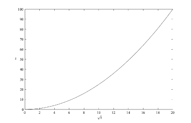
This inversion of abscissa and ordinate in the permits to represent this graph as a line tangent to the classical straight line and hence to have a better graphical picture. Finally, note that if is a standard real, then and the is a vertical line passing through .
The following theorem permits to represent geometrically the Fermat reals
Theorem 35.
If , then the function
is injective. Moreover if , , then we can find (depending on and ) such that
if and only if
| (33) |
Proof: The application for is well defined because it depends on the terms , and of the decomposition of (see Theorem 5 and Definition 8). Now, suppose that , then
| (34) |
Let us consider the Fermat reals generated by these functions, i.e.
then the decompositions of and are exactly the decompositions of and
| (35) | ||||
| (36) |
But from (34) it follows in , and hence also from (35) and (36).
Now suppose that , then, using the same notations of the previous part of this proof, we have also and and hence
We apply Theorem 28 obtaining that locally , i.e.
This is an equivalent formulation of (33), and, because of Theorem 28 it is equivalent to .
Example.
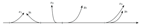
In figure 2 we have the representation of some first order infinitesimals.
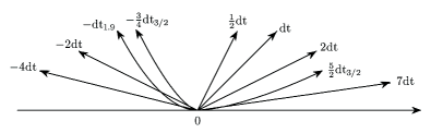
The arrows are justified by the fact that the representing function (32) is defined on and hence has a clear first point and a direction. The smaller is and the nearer is the representation of the product , to the vertical line passing through zero, which is the representation of the standard real . Finally, recall that if and only if .
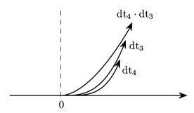
If we multiply two infinitesimals we obtain a smaller number, hence one whose representation is nearer to the vertical line passing through zero, as represented in figure 3
In figure 4 we have a representation of some infinitesimals of order greater than . We can see that the greater is the infinitesimal (with respect to the order relation defined in ) and the higher is the order of intersection of the corresponding line .
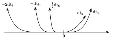
Intuitively, the method to see if is to look at a suitably small neighborhood (i.e. at a suitably small ) at of their representing lines and : if, with respect to the horizontal directed straight line, the curve comes before the curve , then is less than .
XIV Some elementary examples
The elementary examples presented in this section want to show, in a few rows, the simplicity of the algebraic calculus of nilpotent infinitesimals. Here “simplicity” means that the dialectic with the corresponding informal calculations, used e.g. in engineering or in physics, is really faithful. The importance of this dialectic can be glimpsed both as a proof of the flexibility of the new language, but also for researches in artificial intelligence like automatic differentiation theories (see e.g. Griewank (2000) and references therein). Last but not least, it may also be important for didactic or historical researches. Several examples are directly taken from analogous of Bell (1998) and the reader is strongly invited to compare the two theories in these cases. In particular, in our point of view, is not positive, like in some parts of Bell (1998), to return back to a non rigorous use of infinitesimals. Mathematical theories of infinitesimals, like our ring of Fermat reals or NSA or SIA, are great opportunities to avoid several fallacies of the informal approach (our discussion in Section X is a clear example), and to advance further, with the new knowledge originating from the rigorous theory, opening the possibility to use infinitesimal methods in more general, and less intuitive, frameworks (like e.g. infinite dimensional spaces of mappings, see Giordano (2009)). Once again, the key point is the dialectic between formal and informal thoughts and not a single part only.
XIV.1 The heat equation.
In this and the following section we simply use the language of to reformulate the corresponding deductions of Vladimirov (1987). Let us consider a body (identified with its localization) and denote with its interior. On are given the smooth functions , and , interpreted respectively as the mass density, the specific heat capacity and the coefficient of thermal conductivity. Let us note that assuming these functions as defined on without any favored direction corresponds physically to assume that is an isotropous body. Moreover, let be the smooth function representing the temperature of the body at each point and time . To deduce the heat diffusion equation we fix an internal point and an infinitesimal volume . More precisely, we say that a subset of of the form
| (37) |
is an infinitesimal parallelepiped if , i.e. if the corresponding volume is an infinitesimal of some order. Here is the natural base of and notations of the form are only useful to underline that the infinitesimal increment is associated to the variable : here is not an operator and we use it instead of the common to avoid confusion with our introduced in Definition 8. Because , the inclusion follows, so that can be thought as the sub-body of corresponding to the infinitesimal parallelepiped parallel to coordinate axis and centered at . This sub-body interacts thermally with its complement and with external sources of heat. In the infinitesimal time interval , the sub-body exchanges with its complement the heat flowing perpendicularly to the surface of (Fourier’s law):
| (38) |
where and . Choosing the infinitesimals so that
we have that from Theorem 12 (e.g. we can choose and ). From this and the use of infinitesimal Taylor’s formula in (38), simple calculations give
| (39) |
Of course, this calculations correspond to the infinitesimal version of the Gauss-Ostrogradskij theorem. Interacting thermally with external sources, the sub-body exchanges the heat
| (40) |
where is a smooth function representing the intensity of the thermal sources. The total heat corresponds to an increasing of temperature of equal to and hence to an exchange of heat with the environment equal to
| (41) |
From this and (39), (40), the infinitesimal Taylor’s formula and the cancellation law we obtain the conclusion:
To stress that the previous deduction is now completely rigorous we can now state the following theorem, without any mention to the physical interpretation:
Theorem 36.
Unfortunately, this statement does not sufficiently underline the great difference that takes place between the physical content in the definition of , i.e. the Fourier’s law, and that in the definition of . In an axiomatic framework for thermodynamics (see e.g. Truesdell (1991)), the notion of heat flux going from a body to a body can be taken as primitive; in that case (38) becomes an important assumption, whereas (40) is simply the definition of the intensity .
XIV.2 Electric dipole.
In elementary Physics, an electric dipole is usually defined as “a pair of charges with opposite sign placed at a distance very less than the distance from the observer”. Conditions like are frequently used in Physics and very often we obtain a correct formalization if we ask infinitesimal but , i.e. finite. Thus we can define an electric dipole as a pair of electric particles, with charges of equal intensity but with opposite sign such that their mutual distance at every time is a first order infinitesimal:
| (42) |
In this way we can calculate the potential at the point using the properties of and using the hypothesis that is finite and not zero. In fact we have
and if then
because for (42) . For our hypotheses on and we have that hence from the derivation formula
In the same way we can proceed for , hence:
The property is also used in the calculus of the electric field and for the moment of momentum.
XIV.3 Newtonian limit in Relativity.
Another example in which we can formalize a condition like using the previous ideas is the Newtonian limit in Relativity; in it we can suppose to have
-
•
-
•
where is the matrix of the Minkowski’s metric. This conditions can be interpreted as and (low speed with respect to the speed of light and weak gravitational field). In this way we have, e.g. the equalities:
XIV.4 Linear differential equations.
Let
be a linear differential equation with constant coefficients. Once again we want to discover independent solutions in case the characteristic polynomial has multiple roots e.g.
The idea is that in we have also if with . Thus is a solution too. But , hence
We obtain , that is must be a solution. Using -th order infinitesimals we can deal with other multiple roots in a similar way.
XIV.5 Circle of curvature.
A simple application of the infinitesimal Taylor’s formula is the parametric equation for the circle of curvature, that is the circle with second order osculation with a curve . In fact if and is a unit vector, from the second order infinitesimal Taylor’s formula we have
| (43) |
where is the unit normal vector, is the tangent one and the curvature. But once again from Taylor’s formula we have and Now it suffices to substitute and from these formulas into (43) to obtain the conclusion
In a similar way we can prove that any can be written as
so that now the idea of the Fourier series comes out in a natural way.
XIV.6 Commutation of differentiation and integration.
This example derives from Kock (1981); Lavendhomme (1996). Suppose we want to discover the derivative of the function
where , and are smooth functions. We can see as a composition of smooth functions, hence we can apply the derivation formula, i.e. Theorem 21:
Now we use to obtain e.g. (see Corollary 23):
and
Calculating in an analogous way similar terms we finally obtain the well known conclusion. Note that the final formula comes out by itself so that we have “discovered” it and not simply we have proved it. From the point of view of artificial intelligence or from the didactic point of view, surely this discovering is not a trivial result.
XIV.7 Schwarz’s theorem.
Using nilpotent infinitesimals we can obtain a simple and meaningful proof of Schwarz’s theorem. This simple example aims to show how to manage some differences between our setting and SDG. Let be a function between spaces of type , and , we want to prove that is symmetric. Take
(e.g. we can take so that , see also Theorem 12). Using , we have
| (44) |
where we used the fact that and infinitesimal imply . Now we consider that so that any product of type is zero for every , so we obtain
| (45) |
But and hence
Substituting this in (45) and hence in (44) we obtain
| (46) |
The left hand side of this equality is symmetric in , hence changing them we have
and thus we obtain the conclusion because and , . From (46) it follows directly the classical limit relation
XIV.8 Area of the circle and volumes of revolution.
A more or less meaningful proof of the familiar formula for the area of a circle depends on what axioms are assumed and how much general the definitions are. In this example we want to show the possibility to define suitable smooth functions using an infinitesimal property. Let us assume the axioms for the real field ; prove from them the existence of the smooth functions and ; define as a suitable zero of these functions (see e.g. Prodi (1970); Silov (1978)) and define the length of an arc of circle of radius , parametrized by and , as the unique function that verifies
| (47) | ||||
| (48) |
This definition can be justified in the usual way using a (second order!) infinitesimal right-angled triangle. The uniqueness of follows from (47) and (48), the smoothness of and , the second order infinitesimal Taylor’s formula and the cancellation law (Theorem 17):
From this and (48) we obtain the usual formula for that, in our particular case, gives . Now we can think the area of a first order infinitesimal sector of the circle as the area of the isosceles triangle with sides of length and base . In fact, if , then , where is the tangent vector, so that in , , the circle is made of linear segments. Therefore, the area can be defined as the unique function that verifies
From this and the derivation formula we get
In our case we get and hence
the searched formula for .
Analogously we can prove the familiar formula for volumes of revolution
of a parametrized curve , ,
around the -axis. Let us define the volume as the unique smooth
function that verifies
| (49) | ||||
| (50) |
for every and . This definition can be intuitively justified saying that the volume of the sector of revolution between and can be calculated as the sum of the cylinder of radius and height plus one half of the difference between the cylinder of radius and height and that of radius radius and the same height. Implicitly, we are using the straightness of the curve in . From (49) and the property we easily obtain that and hence the usual formula using (50).
XIV.9 Curvature.
Let us consider the usual smooth parametrized curve for . Let be the non-oriented angle (i.e. the one defined by the scalar product) between the tangent vector and the unit vector of the -axis, so that
Multiplying this equality by we easily obtain
| (51) |
It is well known that the curvature of at the point can be calculated as the rate of change of the non-oriented angle with respect to an infinitesimal variation in arc length defined by the analogous of (47) and (48). These “rate of changes” can be defined in as the unique (if it exists) standard defined by
Indeed, from the cancellation law, i.e. Theorem 17, there exists at most one such verifying this property. Because of this uniqueness we can also use the notation
| (52) |
These ratios generalize the usual ratios between real numbers (see Giordano (2009) for more details). From (52) and the derivation formula we get whatever we choose. From this and the relation (51) (without using infinitesimals, but using standard differential calculus) we can obtain the usual formula at each point where and .
XIV.10 Stretching of a spring (and center of pressure).
If is a smooth function and we define , then Corollary 23 and a trivial calculation with the derivation formula give
| (53) |
The right-hand side of (53) is interpreted as the average value of in the infinitesimal interval . Analogous equalities can be obtain in the -dimensional case using suitable generalizations of the above cited corollary: e.g. if we have to use
These equalities are used by Bell (1998) to calculate the center of pressure of a plane area and the work done in stretching a spring. The meaningfulness of such examples is however doubtful because they can be summarized saying: assume to have a smooth satisfying (53); deduce from this and from the assumption that . There is no real use of infinitesimals in this type of reasoning in every case where the definition is customary, like in the cited examples.
XIV.11 The wave equation.
The deduction of the wave equation in the framework of Fermat reals is very interesting for two main reasons. Firstly, in the classical deduction (see e.g. Vladimirov (1987)) there are some approximations tied with Hook’s law. Is it possible to make them rigorous using ? Do we gain something using this increased rigour? E.g.: how can we formalize the approximated equalities used in the classical deduction? In what a sense is the wave equation an approximated equality valid for small oscillations only?
Secondly, at the end of our deduction we will stress the physical principles as important mathematical assumptions of a suitable theorem. We are hence naturally taken to ask if these natural assumptions (some of which formulated using the infinitesimals of ) really have a model. In this way, we will see that no standard smooth function can satisfy these hypothesis, but we are forced to consider a non-standard one. E.g. for and is an example of a non-standard smooth function; let us note that it is obtained by the standard smooth function , , , by extension to and fixing one of its variables to a non-standard parameter :
This will motivate strongly the further development of the theory of Fermat reals, in the direction of a more general theory including also these new smooth non-standard functions.
Let us start considering a string making small transversal oscillations around its equilibrium position located on the interval of the axis, for , , . By hypotheses, string’s position is always represented by the graph of a given curve (where and ; in the following, we will always use these notations for intervals to identify the corresponding subsets of , and not of , and we will also use the notation ):
Moreover, the curve is supposed to be injective with respect to the parameter :
so that the order relation on implies an order relation on the support . For every pair of points , on the string at time , we can define the sub-bodies:
corresponding respectively to the parts of the string that follows the point , that precedes the same point and that lies between the point and the point . It is usually implicitly clear that e.g. every sub-body of the form exerts a force on each sub-body with which it is in contact, i.e. of the form or . Moreover, the force that the sub-body exerts on the sub-body verifies the following equalities (see e.g. Truesdell (1991)):
| (54) | ||||
| (55) | ||||
| (56) |
for every pair of points , and every time . Using this formalism, the tension at the point at time can now be defined in the following way
| (57) |
Now, let us consider the infinitesimal sub-body located at time between the points and , where is a generic first order infinitesimal. On this infinitesimal sub-body, mass forces of linear density act, so that Newton’s law can be written as
| (58) |
where is the linear mass density and where, if not otherwise indicated, all the functions are calculated at . Of course, the contact forces appearing in Newton’s law are due to the interaction of the infinitesimal sub-body with other sub-bodies in contact with its border
Using action-reaction principle (56) and the equality (55), with and so that , from (58) we have
Using (54) and the definition (57) of tension we get
| (59) |
Up to this point of the deduction we have not used neither the hypotheses of small oscillations nor that of transversal oscillations. The second one can be easily introduced with the hypotheses
| (60) |
where are the axis unit vectors. Using the notation for the non-oriented angle between the tangent unit vector at the point and the axes (see (51)), the hypotheses of small oscillations can be formalized with the assumption
| (61) |
This will permit to reproduce the classical deduction in the most faithful way (even if, as we will see later, a weaker assumption can be considered). Moreover, in the classical deduction of the wave equation, one considers only curves of the form . In this way from (51) and the derivation formula we have
so that and hence the total length of the string becomes:
| (62) |
By Hook’s law, this justifies that the tension can be assumed to have a constant modulus , not depending neither by the position nor by the time :
| (63) |
A tension parallel to the tangent vector is the second part of the hypothesis about non transversal oscillations of the string. Let us note explicitly that the only standard continuous function verifying the equality is the constant one, so the function has to be understood as a non-standard one; later we will do further considerations about this important point. Projecting the equation (59) on the axis, we obtain
But because is a first order infinitesimal, hence
| (64) |
We cannot use the cancellation law with to obtain the final result, because, as we mentioned above, the function can assume non standard values, so it is time to clarify some points. As mentioned above, there does not exist a standard smooth function verifying all the assumptions or the physical principles we have used. Of course, everything depends by how we formalize the classical informal deduction used in elementary physics: e.g. we have chosen to use an equality sign in (62) instead of an approximated equality; anyway we have to consider that if we use to write (62), then the problem becomes how to make more precise, physically, numerically or mathematically, this approximation; moreover, if we use an approximation sign in (62), then we consistently must use the same sign both in (63) and therefore in the final wave equation. Nevertheless, smooth non standard functions can verify all the hypothesis and physical principles we have considered: e.g. the function is one of these if the maximum amplitude and if is constant, and .
Definition 37.
If and then we say that
iff maps in and for every we can write
| (65) |
for some
where (see Definition 4 for the relation ).
In other words locally a smooth function from to is constructed in the following way:
-
1.
start with an ordinary standard function , with open in and open in . The space has to be thought as a space of parameters for the function ;
-
2.
consider its Fermat extension obtaining ;
-
3.
consider the composition , where is the isomorphism defined by ; we will always use the identification , so we will write simply instead of .
-
4.
fix a parameter as a first variable of the previous composition, i.e. consider . Locally, the map is of this form: .
Because , with , applying the infinitesimal Taylor’s formula to variable for the function it is not hard to prove the following Theorem, that clarifies further the form of these non standard smooth functions, because it states that they can be seen locally as “infinitesimal polynomials with smooth coefficients”:
Theorem 38.
Let and a map. Then it results that
if and only if for every we can write
| (66) |
for suitable:
-
1.
,
-
2.
-
3.
open subset of such that
-
4.
family of .
In other words, every smooth function can be constructed locally starting from some “infinitesimal parameters”
and from ordinary smooth functions
and using polynomial operation only with , …, and with coefficients . Roughly speaking, we can say that they are “infinitesimal polynomials with smooth coefficients. The polynomials variables act as parameters only”.
As it is natural to expect, several notions of differential and integral calculus, including their infinitesimal versions, can be extended to this type of new smooth function (for more details, see the preprint Giordano (2009)), and these results will be presented in future works. In this sense, this deduction of the wave equation motivates strongly the future development of the theory of Fermat reals.
On the other hand, we have to understand what type of cancellation law we can apply to (64). For this end, we have to define the notion of equality up to -th order infinitesimals:
Definition 39.
Let be the decomposition of and , then
Finally if , , we will say iff in , and we will read it as is equal to up to -th order infinitesimals.
In other words, as it is easy to prove, we have
Therefore, if we denote with
the set of all the infinitesimal of order less that or equal (let us note that ), then we have that if and only if . Equality up to -th order infinitesimal is of course an equivalence relation and preserves all the ring operations of . More in general these equalities are preserved by smooth functions :
Using this notion, it is not hard to prove the following cancellation law up to -th order infinitesimals.
Theorem 40.
Let , , and . Moreover let us consider defined by
| (67) |
then
-
1.
-
2.
If for every , then
It is also interesting to note that not only small oscillations of the string implies (69), but the converse is also true: the equation (69) implies that necessary we must have small oscillations of the string, i.e. that . Moreover, using the equality up to second order infinitesimals, all the classical approximation tied with Hook’s law, now become more clear. Indeed, we have the following
Theorem 41.
Let , , with ; let , and be non standard smooth functions and be an invertible Fermat real. Let us suppose that the first component of the curve is of the form
| (70) |
with . Then the unit tangent vector to the curve exists and we can further suppose that the relations
| (71) | ||||
| (72) |
holds for a every point and for every . Finally, let us suppose that
Then at this point the following sentences are equivalent
-
1.
-
2.
.
Finally, if (2) holds for every , then
To simplify the proof of this result, we need two lemmas.
Lemma 42.
Let , with and let , be non standard smooth functions such that
Then
Lemma 43.
Let , , and suppose that is invertible and , then the following properties are equivalent:
-
1.
-
2.
.
Proof of Theorem 41: We firstly note that, assuming (70), the tangent vector always exists in . In fact we have so that both and are invertible; we can hence take its square root and then the inverse to define the unit tangent vector. Now we prove that (1) implies (2). Let us take a generic . Projecting (72) on we get
But from (71) and because smooth operations preserve , we get . Therefore, from Lemma 42 we obtain
| (73) |
On the other hand, we can multiply (1) by (so that becomes , see Theorem 40) obtaining
| (74) |
Equating (73) and (74) and canceling we get
| (75) |
where, as usual, every function, if not otherwise indicated, is calculated at . Let us note that, in (75) we have used the property because and ; moreover, from (51) if we would have , which is impossible because . Setting, for simplicity, , from (75) and canceling , we have
| (76) |
By Lemma 43 this implies the conclusion.
Vice versa, if is an infinitesimal of order less than or equal 4, then by Lemma 43 we obtain (76) and we can go over again the previous passages in the opposite direction to prove (1).
Now, let us suppose that for every , then
| (77) |
because and hence . But , so
because and and hence . Substituting this in (77) and using the derivation formula for the function we obtain
Therefore
| (78) |
Using the Theorem 38 it is not hard to prove that the last integral in (78) is an infinitesimal of order less than or equal 2, so the conclusion follows from the hypothesis .
Proof of Lemma 42: First of all, from the hypothesis for every , we get that
| (79) |
Now, let us fix a point . From Theorem 38 we obtain that we can write
for every and where , and , are ordinary smooth functions defined in an open neighbourhood of . From (79) we have for every so that on and hence also on . Therefore
| (80) |
This difference must have order less than or equal 2 because , so
Let us suppose, for simplicity, that is this term of maximum order. Because it must be that and hence also and . Finally we have
but because and because and ; we hence obtain
Proof of Lemma 43: If , then the standard parts of both sides must be equal
By hypotheses is invertible, hence and we obtain that because , i.e. . Moreover, from infinitesimal Taylor’s formula applied to , and from we obtain
where and are invertible Fermat reals. From this we get and hence , i.e. and hence .
Vice versa, if is an infinitesimal of order less than or equal 4 (so that if ) we have
Therefore, so that is an infinitesimal of order , i.e. .
The reader with a certain knowledge of SDG had surely noted that this deduction of the wave equation cannot be reproduced in SDG because of the use of non standard smooth functions, of the use of equalities up to -th order infinitesimals and because of the frequent use of the useful Theorem 12 to decide products of powers of nilpotent infinitesimals.
XV Conclusions
The problem to turn informal infinitesimal methods into a rigorous theory has been faced by several authors. The most used theories, i.e. NSA and SDG, require a good knowledge of Mathematical Logic and a strong formal control. Some others, like Weil functors (see e.g. Kriegl and Michor (1996)) or the Levi-Civita field (see e.g. Shamseddine (1999)) are mainly based on formal/algebraic methods and sometimes lack the intuitive meaning. In this initial work, we have shown that it is possible to bypass the inconsistency of SIA with classical logic modifying the Kock-Lawvere axiom (see e.g. Lavendhomme (1996)) and keeping always a very good intuitive meaning. We have seen how to define the algebraic operations between this type of nilpotent infinitesimals, infinitesimal Taylor formula and order properties. In the final part we have seen several elementary examples of the use of these infinitesimals, some of them taken from classical deductions of elementary Physics. In our opinion, these examples are able to show that some results that frequently may appear as unnatural in a standard context, using Fermat reals can be discovered, even by suitably designed algorithm. Moreover, our generalization of the classical proof of the wave equation have shown that a rigorous theory of infinitesimals permits to obtain results that are not accessible using only an intuitive approach.
References
- Albeverio et al. [1988] S. Albeverio, J.E. Fenstad, R. Høegh-Krohn, and T. Lindstrøm. Nonstandard Methods in Stochastic Analysis and Mathematical Physics. Pure and Applied Mathematics. Academic Press, 1988. 2nd ed., Dover, 2009.
- Bell [1937] E.T. Bell. Men of Mathematics. Simon and Schuster, New York, 1937.
- Bell [1998] J.L. Bell. A Primer of Infinitesimal Analysis. Cambridge University Press, 1998.
- Benci and Di Nasso [2003] V. Benci and M. Di Nasso. A ring homomorphism is enough to get nonstandard analysis. Bull. Belg. Math. Soc. - S. Stevin, 10:481–490, 2003.
- Benci and Di Nasso [2005] V. Benci and M. Di Nasso. A purely algebraic characterization of the hyperreal numbers. Proceedings of the American Mathematical Society, 133(9):2501–05, 2005.
- Bertram [2008] W. Bertram. Differential Geometry, Lie Groups and Symmetric Spaces over General Base Fields and Rings. American Mathematical Society, Providence, 2008.
- Berz [1994] M. Berz. Analysis on a Nonarchimedean Extension of the Real Numbers. Mathematics Summer Graduate School of the German National Merit Foundation, MSUCL-933, Department of Physics, Michigan State University, 1992 and 1995 edition, 1994.
- Bröcker [1975] T. Bröcker. Differentiable germs and catastrophes, volume 17 of London Mathematical Society Lecture Note Series. Cambridge University Press, Cambridge, 1975.
- Conway [1976] J.H. Conway. On Numbers and Games. Number 6 in L.M.S. monographs. Academic Press, London & New York, 1976.
- Dirac [1975] P.A.M. Dirac. General Theory of Relativity. John Wiley and Sons, 1975.
- Edwards [1979] C.H. Edwards. The Historical Development of the Calculus. Springer-Verlag, New York, 1979.
- Ehresmann [1951] C. Ehresmann. Les prolongements d’une variété différentiable: Calculus des jets, prolongement principal. C. R. Acad. Sc. Paris, 233:598–600, 1951.
- Einstein [1926] A. Einstein. Investigations on the Theory of the Brownian Movement. Dover, 1926.
- Eves [1990] H. Eves. An Introduction to the History of Mathematics. Saunders College Publishing, Fort Worth, TX, 1990.
- Giordano [2004] P. Giordano. Infinitesimal differential geometry. Acta Mathematica Universitatis Comenianae, LXIII(2):235–278, 2004.
- Giordano [2009] P. Giordano. Fermat reals: Nilpotent infinitesimals and infinite dimensional spaces. arXiv:0907.1872, July 2009.
- Golubitsky and Guillemin [1973] M. Golubitsky and V. Guillemin. Stable mappings and their singularities, volume 14 of Graduate texts in mathematics. Springer, Berlin, 1973.
- Griewank [2000] A. Griewank. Evaluating Derivatives: Principles and Techniques of Algorithmic Differentiation, volume 19 of Frontiers in Applied Mathematics. SIAM, 2000.
- Henson [1997] C.W. Henson. Foundations of nonstandard analysis. a gentle introduction to nonstandard extension. In L.O. Arkeryd, N.J. Cutland, and C.W. Henson, editors, Nonstandard analysis: theory and applications (Edinburgh, 1996), pages 1–49, Dordrecht, 1997. NATO Adv. Sci. Inst. Ser. C: Math. Phys. Sci., vol. 493, Kluwer Acad. Publ.
- Kock [1981] A. Kock. Synthetic Differential Geometry, volume 51 of London Math. Soc. Lect. Note Series. Cambridge Univ. Press, 1981.
- Kriegl and Michor [1996] A. Kriegl and P.W. Michor. Product preserving functors of infinite dimensional manifolds. Archivum Mathematicum (Brno), 32, 4:289–306, 1996.
- Lavendhomme [1996] R. Lavendhomme. Basic Concepts of Synthetic Differential Geometry. Kluwer Academic Publishers, Dordrecht, 1996.
- Moerdijk and Reyes [1991] I. Moerdijk and G.E. Reyes. Models for Smooth Infinitesimal Analysis. Springer, Berlin, 1991.
- Prodi [1970] G. Prodi. Analisi matematica. Ed. Bollati Boringhieri, Torino, 1970.
- Shamseddine [1999] K. Shamseddine. New Elements of Analysis on the Levi-Civita Field. PhD thesis, Michigan State University, East Lansing, Michigan, USA, 1999.
- Silov [1978] G.E. Silov. Analisi matematica. Funzioni di una variabile (it. transl.). Mir, Mosca, 1978.
- Truesdell [1991] C. Truesdell. A First Course in Rational Continuum Mechanics: v.1 General Concepts, 2nd ed., volume 71 of Pure and Applied Mathematics. Academic Press Inc., 1991.
- Vladimirov [1987] V.S. Vladimirov. Equazioni della fisica matematica. MIR, 1987.