The quenched-disordered Ising model in two and four dimensions

Abstract

We briefly review the Ising model with uncorrelated, quenched random-site or random-bond disorder, which has been controversial in both two and four dimensions. In these dimensions, the leading exponent $\alpha$, which characterizes the specific-heat critical behaviour, vanishes and no Harris prediction for the consequences of quenched disorder can be made. In the two-dimensional case, the controversy is between the strong universality hypothesis which maintains that the leading critical exponents are the same as in the pure case and the weak universality hypothesis, which favours dilution-dependent leading critical exponents. Here the random-site version of the model is subject to a finite-size scaling analysis, paying special attention to the implications for multiplicative logarithmic corrections. The analysis is fully supportive of the scaling relations for logarithmic corrections and of the strong scaling hypothesis in the 2D case. In the four-dimensional case unusual corrections to scaling characterize the model, and the precise nature of these corrections has been debated. Progress made in determining the correct 4D scenario is outlined.

1 Introduction

Continuous phase transitions are characterized by critical exponents. In terms of the reduced temperature $t$ and the reduced external magnetic field $h$, which are measures of how far the system is from its critical point $(t,h)=(0,0)$, the standard power-law leading behaviour is as follows:

$${\mbox{specific heat at $h=0$:}}\quad\quad\quad\quad\quad\quad\quad\quad\quad~{}~{}~{}c_{\infty}(t) \sim |t|^{-\alpha}\,,$$ (1)

$${\mbox{spontaneous magnetization at $h=0$, $t<0$:}}\quad m_{\infty}(t) \sim |t|^{\beta}\,,$$ (2)

$${\mbox{susceptibility at $h=0$:}}\quad\quad\quad\quad\quad\quad\quad\quad~{}~{}~{}~{}~{}\chi_{\infty}(t) \sim |t|^{-\gamma}\,,$$ (3)

$${\mbox{magnetization at $t=0$:}}\quad\quad\quad\quad\quad\quad\quad\quad~{}~{}~{}m_{\infty}(h) \sim |h|^{\frac{1}{\delta}}\,,$$ (4)

$${\mbox{correlation length at $h=0$:}}\quad\quad\quad\quad\quad\quad\quad~{}\,\,\,\xi_{\infty}(t) \sim |t|^{-\nu}\,.$$ (5)

The subscripts here represent the linear extent of the system. The correlation function at criticality decays as

$${\cal{G}}_{\infty}(x)=x^{-(d-2+\eta)}\,,$$ (6)

where $x$ represents distance along the lattice, the dimensionality of which is $d$. These six critical exponents are related by four scaling relations, namely

$$\nu d = 2-\alpha\,,$$ (7)

$$2\beta+\gamma = 2-\alpha\,,$$ (8)

$$\beta(\delta-1) = \gamma\,,$$ (9)

$$\nu(2-\eta) = \gamma\,.$$ (10)

If a pure system (i.e., a system defined on a regular intact lattice) is characterized by a particular set of critical exponents, it is interesting to ask what happens to this set if randomization is introduced to the lattice sites or bonds. The quenched random removal of sites or the randomization of bond strengths is believed to immitate the presence of impurities in real physical systems, so this question is relevant for meaningful comparison with experiments.

In most cases the Harris criterion provides an answer to this question Ha74 . If $\alpha>0$ in the pure system, quenched disorder is relevant and the critical exponents change as such disorder is added. If, on the other hand, $\alpha<0$ in the pure model, then this type of disorder does not alter critical behaviour and the critical exponents are unchanged upon randomizing the lattice structure. The Harris criterion does not, however, provide aa clear an answer in the circumstance where specific-heat critical exponent $\alpha$ vanishes in the pure model, as is the case for the Ising model in both two and four dimensions. As a result, these circumstances have been quite controversial. In the following two sections the histories and natures of the controversies in 2D and 4D are outlined. An approach to tackle these subtle issues is presented in the following section where the results of applications of this method to both cases are also presented. Conclusions are drawn in the final section.

2 The two-dimensional case

In the same manner as the pure Ising model in two dimensions can be formulated as a lattice theory of free fermions, the randomized model can be formulated as a theory of interacting fermions. This interaction can be considered perturbatively about the solvable pure case. In DD Dotsenko and Dotsenko used a truncated form of Grassmann field theory together with the replica trick, to link the problem to the $N=0$ Gross-Neveu model. They derived the following behaviour for the specific heat in the RBIM:

$$c_{\infty}(t)\sim\ln{|\ln{|t|}|}\,.$$ (11)

They also derived an expression for the scaling behaviour of the susceptibility, namely $\chi_{\infty}(t)\sim t^{-2}\exp{(-c|\ln{|\ln{|t|}|}|^{2})}$, where $c$ is a constant. Their value $\gamma=2$ there was different to that in the pure theory (which has $\gamma=7/4$) and the notion that the leading critical exponents may change when going from the pure to the random 2D Ising model became known as the weak universality hypothesis. In fact, the notion of weak universality as advanced by Suzuki Su74 is that some exponents may change with dilution, but combinations which appear in terms of the correlation length (e.g., in $\chi_{\infty}(t)\sim\xi_{\infty}^{\gamma/\nu}(t)$) are dilution independent. I.e., $\beta/\nu$and $\gamma/\nu$ are unchanged (as are $\delta$ and $\eta$).

In GJ83 , Jug derived two-loop renormalization-group (RG) results in the 2D (and 3D) RSIM. (For a recent review on the 3D RSIM, see FoHo03 .) He also worked out the exact RG and $\epsilon$-expansion along the curve in $(n,d)$-space where the pure system’s specific-heat $\alpha$-exponent vanishes. Here $n$ is the number of components of the order parameter in $O(n)$ models. This includes the $n=1$ RSIM case in $d=2$ (as well as $d=4$, which we shall discuss in the next section). For the 2D case, he showed that the critical behaviour is controlled by the pure-model fixed point, so that the leading exponents are the same as in the pure case. In particular, and contrary to the susceptibility results of DD , Jug’s approach gave $\gamma=7/4$ for the diluted model – which is the same value as in the pure case. The notion that the leading critical exponents are unchanged by randomizing the lattice structure became known as the strong universality hypothesis.

For $d=2$, Jug also derived a change in the logarithmic form of the heat capacity, either to $|\ln|t||^{\hat{\alpha}}$ with $\hat{\alpha}={\cal{O}}(\epsilon)$ or $\ln{|\ln{|t|}|}$ if $\hat{\alpha}=0$ GJannouncement . In GJ84 , Jug confirmed the result (11) for the heat capacity for the 2D RBIM using Grassmann field theory. On the basis of the chronology outlined above, we refer to the (now famous) proposed behaviour (11) in the specific heat as the Dotsenko-Dotsenko-Jug (DDJ) double logarithm.

Shalaev later introduced bosonization to the above approaches and derived that all critical exponents are the same as in the pure case but there are, in fact, non-trivial multiplicative logarithmic corrections to the susceptibility and correlation length in the RBIM Boris2D . He derived the exponents of these logarithms and again obtained the double logarithm of the specific heat, results which were later re-obtained by Shankar and Ludwig SL . Using transfer matrix techniques together with the self-duality of the RBIM, and the replica trick, to map the model to the $O(N)$ Gross-Neveu model, to which RG is applied to one loop, Jug and Shalaev later derived the logarithmic corrections for the remaining quantities in the RBIM JuSh96 .

Modifying the standard scaling expressions (1)–(6), above, to include multiplicative logarithmic corrections, we write the universal scaling forms

$$c_{\infty}(t) \sim |t|^{-\alpha}|\ln{|t|}|^{\hat{\alpha}}\,,$$ (12)

$$m_{\infty}(t) \sim |t|^{\beta}|\ln{|t|}|^{\hat{\beta}}\,,$$ (13)

$$\chi_{\infty}(t) \sim |t|^{-\gamma}|\ln{|t|}|^{\hat{\gamma}}\,,$$ (14)

$$m_{\infty}(h) \sim h^{\frac{1}{\delta}}|\ln{|h|}|^{\hat{\delta}}\,.$$ (15)

$$\xi_{\infty}(t) \sim |t|^{-\nu}|\ln{|t|}|^{\hat{\nu}}\,,$$ (16)

$${\cal{G}}_{\infty}(x) \sim x^{-(d-2+\eta)}(\ln{x})^{\hat{\eta}}\,.$$ (17)

Allowing also for the possibility of logarithmic corrections to the FSS behaviour of the correlation length, we also write the universal scaling form

$$\xi_{L}(0)\sim L(\ln{L})^{\hat{q}}\,.$$ (18)

A set of universal scaling relations for the correction exponents has recently been developed which connects the universal hatted exponents in a manner analogous to (7)–(10). These are KeJo06a ; KeJo06b

$$\hat{\alpha} = \left\{{\begin{array}[]{l}~{}1+d\hat{q}-d\hat{\nu}\quad{\mbox{if}}\quad\alpha=0\quad{\mbox{and}}\quad\phi\neq\pi/4\\ ~{}d\hat{q}-d\hat{\nu}\,\quad{\mbox{otherwise,}}\end{array}}\right.$$ (21)

$$2\hat{\beta}-\hat{\gamma} = d\hat{q}-d\hat{\nu}\,,$$ (22)

$$\hat{\beta}(\delta-1) = \delta\hat{\delta}-\hat{\gamma}\,,$$ (23)

$$\hat{\eta} = \hat{\gamma}-\hat{\nu}(2-\eta)\,.$$ (24)

In the first of these, $\phi$ refers to the angle at which the complex-temperature zeros impact onto the real axis. If $\alpha=0$, and if this impact angle is any value other than $\pi/4$, an extra logarithm arises in the specific heat. This is expected to happen in $d=2$ dimensions, but not in $d=4$, where $\phi=\pi/4$ KeJo06b . In KeJo06b it was also shown that

$$\mbox{if}\quad\alpha=0\quad\mbox{and if}\quad d(\hat{\nu}-\hat{q})=1\,,$$ (25)

then the specific heat necessarily has the double-logarithmic divergence (11).

The Jug-Shalaev-Shankar-Ludwig (JSSL) values for the leading critical exponents and for their logarithmic counterparts are

$$\alpha=0\,,\quad\beta=\frac{1}{8}\,,\quad\gamma=\frac{7}{4}\,,\quad\delta=15\,,\quad\nu=1\,,\quad\eta=\frac{1}{4}\,,$$ (26)

$$\hat{\alpha}=0\,,\quad\hat{\beta}=-\frac{1}{16}\,,\quad\hat{\gamma}=\frac{7}{8}\,,\quad\hat{\delta}=0\,,\quad\hat{\nu}=\frac{1}{2}\,,\quad\hat{\eta}=0\,.$$ (27)

The observation that the set of leading exponents (26) obeys the usual scaling relations (7)–(10) is a trivial one, since they are identical to those of the pure Ising model in $d=2$. More interesting is the observation that, with $\hat{q}=0$, de95 ; de97Lede06 ; Aade97StAa97 ; Aade96 , the JSSL correction exponents (27) obey the scaling relations for logarithmic corrections (21)–(24). The observation that they also obey (25) with $\hat{q}=0$, leads to a new route to the derivation of the DDJ double logarithm in the specific heat KeJo06b .

Analytically and numerically based alternatives to the JSSL scenario and to the DDJ double logarithm in the specific heat have been made in the literature. Timonin commented that the replica trick, which was employed in the previous analytical approaches, encounters a problem in that RG is only valid with 1 or 2 replicas, preventing the necessary $n\rightarrow 0$ limit Ti89 . Using Grassmannian methods and perturbative RG (with certain other assumptions but without replicas) he derived $\hat{\alpha}=-1/2$, i.e., a finite specific heat, in the RBIM. Ziegler used a supersymmetric formulation, where $n=0$ is replaced by $N$ bosons and $2N$ fermions to give a non-perturbative approach to show that the specific heat does not, in fact, diverge in the RSIM Zi88 and RBIM Zi91 . Besides the work of Jug, this was the only analytic work on the RSIM to this point. Finally, in 1998, Plechko Pl98 used Grassmann lattice theory to give theoretical support for the double logarithm in the RSIM.

To summarize, both the RSIM and the RBIM have been targeted over many years using a plethora of analytical approaches, some of which support the weak universality hypothesis and others of which support strong universality. In order to discriminate between the two, and to decide whether or not the specific heat diverges in these models, there have also been many numerical investigations of the problem.

Early numerical work by Zobin was supportive of the strong hypothesis in the RBIM in that the susceptibility exponent $\gamma$ was found to be unchanged there Zo78 . In 1990, Andreichenko, Dotsenko, Selke and Wang AnDo90WaSe90TaSh94 used such a numerical approach to present evidence in support of the strong hypothesis. They focused on the RBIM because the self-duality of that model leads to an exact value for the critical temperature $T_{c}$, ameliorating some aspects of the numerical analyses. Since then many numericists claim support for the strong hypothesis and the double logarithm in the specific heat, mostly for the RBIM, but also for the RSIM. However many others support the weak hypothesis and a finite specific heat (mostly for the RSIM, but also for the RBIM). The situation is summarized in Table 1.

		RBIM	RSIM
Support strong universality hypothesis		de97Lede06 ; Aade96 ; Zo78 ; RoAd98 ; BeCh04 ; SzIg99LaIg00	Se94 ; deSt94 ; ShVa01
	and theoretical support for $\alpha=\hat{\alpha}=0$	DD ; GJ84 ; Boris2D ; SL ; JuSh96 ; KeJo06b	GJ83 ; GJannouncement ; KeJo06b ; Pl98
	or numerical support for $\alpha=\hat{\alpha}=0$	Aade97StAa97 ; AnDo90WaSe90TaSh94 ; HaTo08 ; WiDo95 ; FyMa08	HaTo08 ; BaFe97 ; SeSh98
Support for weak universality hypothesis		Ki95	FaHo92
	and theoretical support for finite $C_{\infty}(t)$	Zi91 ; finiteCinBond	Zi88
	or numerical support for finite $C_{\infty}(t)$	Ki00b ; Ki00	He92 ; KiPa94 ; Ku94KuMa00 ; HaMa08

Table 1: Recent works supportive of the weak or strong scaling hypothesis and for and against the double logarithm in the specific heat in the RBIM and RSIM in $d=2$ dimensions.

While Roder et al. presented strong numerical evidence that $\hat{\gamma}=7/8$ in the RBIM RoAd98 , their series-expansion approach did not lead to a clear result for the specific heat, and almost any reasonable value $\hat{\alpha}\leq 1$ could be supported from their data. Indeed, it was emphasised in Ki00b that plots of the type contained in Refs. AnDo90WaSe90TaSh94 ; HaTo08 for the RBIM and in Refs. HaTo08 ; BaFe97 ; SeSh98 for the RSIM, which purport to display double-logarithmic behaviour of the specific heat do not actually imply such divergence. I.e., it is very difficult (even impossible) to distinguish between

$$c_{\infty}(t)\sim A+B\ln{|\ln{|t|}|}\quad{\mbox{and}}\quad c_{\infty}(t)\sim A-B|t|^{-\alpha}\quad{\mbox{or}}\quad c_{\infty}(t)\sim A-B|\ln{|t|}|^{\hat{\alpha}}\,,$$ (28)

with $\alpha<0$ or $\hat{\alpha}<0$, on the basis of direct numerical simulations of the specific heat. Numerically based counter-claims for the latter two behaviours (so that the specific heat remains finite) in the random-bond Ki00b ; Ki00 and random-site models He92 ; KiPa94 ; Ku94KuMa00 ; HaMa08 also exist.

Thus, like the analytical situation, the numerical approaches to the equilibrium lattice-disordered Ising models in 2D have generated much controversy and debate. (For non-equilibrium scaling aspects in these types of models, see HePl08 .) While it is perhaps fair to say that the strong hypothesis is mostly favoured, agreement is not universal. Also, the double logarithmic behaviour of the specific heat has resisted attempts at verification because of the difficulties in disentangling the scenarios of Eq.(28).

Here we present a method which circumvents these difficulties. We use the recently developed scaling relations for logarithmic corrections KeJo06a ; KeJo06b to express the scaling of Lee-Yang zeros (in particular their density) in terms of the specific heat exponents $\alpha$ and $\hat{\alpha}$. Since the density of zeros is not accompanied by a constant or homogeneous term, it provides a cleaner Ansatz with which to extract $\alpha$ and $\hat{\alpha}$ numerically, at least in the $d=2$ case.

3 The four-dimensional case

Since the upper critical dimensionality of the RSIM, like its pure counterpart, is $d=4$, the leading critical exponents are given by mean field theory

$$\alpha=0\,,\quad\beta=\frac{1}{2}\,,\quad\gamma=1\,,\quad\delta=3\,,\quad\nu=\frac{1}{2}\,,\quad\eta=0\,,\quad\Delta=\frac{3}{2}\,,$$ (29)

and there is no weak universality hypothesis. However, this model is characterised by unusual corrections to scaling together with multiplicative logarithmic terms, the precise nature of which are unsettled.

The consensus in the literature is that the scaling behaviour of the RSIM in four dimensions is given by GJ83 ; Ah76 ; Boris4D ; GeDe93 ; BaFe98 ; HeJa06

$$C_{\infty}(t) \approx A-B|t|^{-\alpha}\exp{\left({-2\sqrt{\frac{6}{53}|\ln{|t|}|}}\right)}|\ln{|t|}|^{\hat{\alpha}}\,,$$ (30)

$$\chi_{\infty}(t) \sim |t|^{-\gamma}\exp{\left({\sqrt{\frac{6}{53}|\ln{|t|}|}}\right)}|\ln{|t|}|^{\hat{\gamma}}\,,$$ (31)

$$\xi_{\infty}(t) \sim |t|^{-\nu}\exp{\left(\frac{1}{2}{\sqrt{\frac{6}{53}|\ln{|t|}|}}\right)}|\ln{|t|}|^{\hat{\nu}}\,.$$ (32)

Modification of the theory presented in KeJo06a gives that the scaling behaviour for the magnetization in this 4D model is

$$m_{\infty}(t) = t^{\beta}\exp{\left({-\frac{1}{2}\sqrt{\frac{6}{53}|\ln{|t|}|}}\right)}|\ln{t}|^{\hat{\beta}}\,,$$ (33)

$$m_{\infty}(h) = h^{\frac{1}{\delta}}|\ln{h}|^{\hat{\delta}}\,.$$ (34)

There is no dispute in the literature regarding the unusual exponential correction terms in (30)–(32), but there are five different sets of predictions for the exponents of the logarithmic terms, which differ from their counterparts in the pure model.

Log exponent	$\hat{\alpha}$	$\hat{\beta}$	$\hat{\gamma}$	$\hat{\delta}$	$\hat{\nu}$	$\hat{\eta}$	$\hat{q}$	$\hat{\Delta}$
Aharony Ah76	0.5	0.25	0	0.167	0	0	0.125	0.25
Shalaev Boris2D	1.237	0.434	-0.368	0.167	-0.189	0.009	0.120	0.803
Jug GJ83	0.5	0.252	0.005	0.170				0.248
Geldart & De’Bell GeDe93	1.246	0.439	-0.368	0.170	-0.187	0.005	0.125	0.807
Ballesteros et al BaFe97	0.5	0.255	0.009	0.173	0	0.009	0.125	0.245

Table 2: Analytic predictions for the logarithmic correction exponents in the 4D RSIM. Entries in boldface come directly from the cited references. The remaining entries come from the scaling relations for logarithmic corrections.

Using RG, Aharony derived the unusual exponential terms in (30)–(32), and Ah76

$$\hat{\alpha}=\frac{1}{2}\,,\quad\hat{\gamma}=0\,,\quad\hat{\nu}=0\,.$$ (35)

In Boris4D , Shalaev refined Aharony’s calculations to higher order in perturbation theory, yielding

$$\hat{\alpha}=1.2368\,,\quad\hat{\gamma}=-0.3684\,,\quad\hat{\eta}=0094\,.$$ (36)

Jug’s calculations along the $\alpha=0$ line in $(n,d)$ space yielded GJ83

$$\hat{\alpha}=1/2\,,\quad\hat{\gamma}=1/212\approx 0.0047\,$$ (37)

at $(n,d)=(1,4)$. In GeDe93 , Geldart and De’Bell derived

$$\hat{\alpha}\approx 1.2463,\quad\hat{\gamma}\approx-0.3684,\quad\hat{\eta}=\frac{1}{212}=0.0047,$$ (38)

and finally Ballesteros et al. BaFe98 gave

$$\hat{\alpha}=\frac{1}{2},\quad\hat{\gamma}=\frac{1}{106}\approx 0.0094,\quad\hat{\nu}=0,\quad\hat{q}=\frac{1}{8}.$$ (39)

From these fragmented pictures, complete scaling scenarios may be built using the scaling relations for logarithmic corrections. These scenarios are summarized in Table 2.

It is remarkable that none of the five analyical works on this model agree regarding the detail of the logarithmic correction exponents, a circumstance which motivated our investigations into the model. We chose to investigate the random-site versions of the models, as this has hitherto proved most controversial in 2D. These investigations use the Lee-Yang zeros of the partition function, which we next describe.

4 A Fresh Perspective: Lee-Yang Zeros

We have examined the RSIM in both two and four dimensions from a fresh perspective, namely using the Lee-Yang zeros of the partition function.

A phase transition is a physical manifestation of a mathematical non-analycity in the free energy. Since the free energy is essentially the logarithm of the partition function, non-analyticities arise when the latter vanishes. Writing the partition function for a system of size $L$ as $Z_{L}(t,h)$, one may consider zeros in either of the variables $t$ or $h$. In each case, the zeros are located in the complex plane. This tack was first suggested by Lee and Yang, and complex-$h$ zeros (which, according to a theorem by the same authors, are usually located along the imaginary $h$-axis) are called Lee-Yang zeros. Above the critical temperature ($t>0$), where there is no phase transition, they are located away from the critical point $h=0$. There, the zeros may be considered to be “proto-critical points”, in the sense that they have the potential to become actual transition points.

4.1 Scaling

The start of the distribution of complex-$h$ zeros in the $t>0$ phase is called the Yang-Lee edge, which we write as $r_{\rm{YL}}(t)$. As the temperature is reduced towards the critical one ($t\rightarrow 0$), the edge and the distribution of zeros move towards the real axis, which they pinch at $t=0$. This pinching, which precipitates the phase transition, scales in a manner characterised by critical exponents. Allowing for logarithmic corrections here too, we write

$$r_{\rm{YL}}(t)\sim t^{\Delta}|\ln{t}|^{\hat{\Delta}}\,,$$ (40)

in the 2D case. For the 4D model, we have to account for the unusual correction terms. Following the theory presented in KeJo06a , it turns out that the scaling behaviour for the Yang-Lee edge is (see also RL )

$$r_{\rm{YL}}(t)\sim t^{\Delta}\exp{\left({-\frac{3}{2}\sqrt{\frac{6}{53}|\ln{|t|}|}}\right)}|\ln{t}|^{\hat{\Delta}}\,.$$ (41)

The exponent $\Delta$ is called the gap exponent. It is related to the other exponents via

$$\Delta=\beta+\gamma\,.$$ (42)

The logarithmic analogue to this scaling relation is KeJo06a

$$\hat{\Delta}=\hat{\beta}-\hat{\gamma}\,.$$ (43)

Besides the scaling behaviour of the Yang-Lee edge, one may also consider the density of zeros, which, for an infinitely large system, we write as $g_{\infty}(r,t)$, where $r$ parametrizes their locus along the imaginary $h$-axis (assuming the Lee-Yang theorem holds). In fact it is more convenient to consider the integrated, or cumulative, distribution function of zeros, which is defined as

$$G_{\infty}(r,t)=\int_{r_{\rm{YL}}(t)}^{r}{g_{\infty}(s,t)ds}\,.$$ (44)

From KeJo06a ; KeJo06b , in the 2D case at $t=0$ this is

$$G_{\infty}(r)\sim r^{\frac{2-\alpha}{\Delta}}(\ln{r})^{\hat{\alpha}-1-(2-\alpha)\frac{\hat{\Delta}}{\Delta}}\,.$$ (45)

Following a similar approach to that oulined in KeJo06a , in the 4D case, one determines

$$G_{\infty}(r)\sim r^{{\frac{2-\alpha}{\Delta}}}\exp{\left({\left({1-\frac{3\gamma}{2\Delta}}\right)\sqrt{\frac{6}{53}|\ln{r}}|}\right)}|\ln{r}|^{\hat{\alpha}-(2-\alpha)\frac{\hat{\Delta}}{\Delta}}\,.$$ (46)

Using the mean-field values $\gamma=1$ and $\Delta=3/2$, the exponential term drops out of this expression.

4.2 Finite-Size Scaling

The finite-size scaling (FSS) behavior for the susceptibility, the Yang-Lee edge and the specific heat for each model is determined by using (16) and (32) to write the reduced temperature in terms of the correlation length. Then the behaviour of the various functions may be expressed directly in terms of $\xi_{\infty}(t)$. For sufficiently large lattices, $\xi_{\infty}(t)$ may be replaced by $\xi_{L}(0)$ at the critical point. The relationship between $\xi_{L}(0)$ and the lattice size is, in turn, given by (18), where ${\hat{q}}=0$ in the 2D case and ${\hat{q}}$ is listed in Table 2 in the 4D scenarios.

The unusual exponential correction terms in 4D, which otherwise swamp the logarithmic corrections, are not in doubt in the literature. To probe the contested logarithmic correction terms, therefore, these terms have to be removed. It turns out that these terms cancel out in the FSS expressions for the susceptibility, the Yang-Lee edge and the density of zeros in the 4D case.

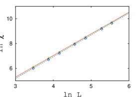
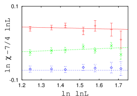
Figure 1: The leading FSS (left) and corrections (right) for the susceptibility in the RSIM in two dimensions for weak ($p=0.88889$, upper data set, red online), moderate ($p=0.75$, middle set, green online) and strong ($p=0.66661$, lower set, blue online) dilution values.

To summarize, the FSS behaviour for the susceptibility and for the edge (i.e., the first Lee-Yang zero) in both models is given by

$$\chi_{L}(0)\sim L^{\frac{\gamma}{\nu}}|\ln{L}|^{\hat{\zeta}} \hat{\zeta}={\frac{\nu{\hat{\gamma}}-\gamma\hat{\nu}+\gamma\hat{q}}{\nu}}\,,$$ where (47)

$$r_{1}(L)\sim L^{-\frac{\Delta}{\nu}}|\ln{L}|^{\hat{\rho}} \hat{\rho}=\frac{\nu\hat{\Delta}+\Delta\hat{\nu}-\Delta\hat{q}}{\nu}\,.$$ where (48)

The FSS of the specific heat in each model is

$$c_{L}(0) \sim (\ln{L})^{\hat{\alpha}}+{\rm{constant}}\quad{\mbox{when}}\quad d=2\,,$$ (49)

$$c_{L}(0) \approx A-B^{\prime}\exp{\left({-2\sqrt{\frac{12}{53}\ln{L}}}\right)}(\ln{L})^{\hat{\alpha}}\quad{\mbox{when}}\quad d=4\,.$$ (50)

In the 2D case, it is difficult to test the Ansatz (49), as explained around Eq.(28). There, we shall instead extract $\hat{\alpha}$ using the form (45) for the density, together with the scaling relations for logarithmic corrections.

5 Numerical Approach

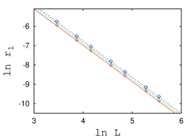
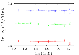
Figure 2: The leading (left) and corrections (right) to FSS for the Yang-Lee edge for the RSIM in 2D for weak ($p=0.88889$, lower data set, red online), moderate ($p=0.75$, middle set, green online) and strong ($p=0.66661$, upper set, blue online) dilution values.

We have simulated the RSIM in both $d=2$ and $d=4$ dimensions using the Wolff single-cluster algorithm Wolff89 . The quenched dilution is implemented by occupying a site at a given point on the lattice with probability $p$, so that $p=1$ corresponds to the pure (intact) model. In the $d=2$ case, we simulated at weak, moderate and strong site-dilution values, represented by $p=0.88889$, $p=0.75$ and $p=0.66661$, respectively, and we used lattices of size $L=32$, 48, 64, 96, 128, 196 and 256. In the $d=4$ case $p=0.8$ and $p=0.5$ with $L=$ 8, 12, 16, 24, 32 and 48 were used. We also simulated the pure $p=1$ models. The simulations were carried out at the critical temperatures estimated in BaFe97 ; BaFe98 and periodic boundary conditions were used. Up to 1000 realizations of disorder were generated for each lattice size and each dilution value, with the specific heat, susceptibility, and lowest zeros being determined for each one. These were then averaged to give estimates for each quenched model. Further details are supplied in KeRu08 ; GoKe09 .

5.1 The Two-Dimensional Case

We begin the analysis with the susceptibility, the FSS for which is given in (47) with the JSSL predictions (26) giving $\gamma/\nu=7/4$. In fact although the weak hypothesis advocates dilution-dependent leading exponents, the ratio $\gamma/\nu$ is believed to be fixed there, so one cannot distinguish between the strong and weak scenarios on this basis. However, Roder et al. have presented compelling evidence for the value $\gamma=7/4$ RoAd98 , which we can input into FSS in order to extract $\nu$. The results of this process are depicted in Fig. 1 and summarized in Table 3. From fits to the leading behaviour $\chi_{L}(0)\sim L^{\gamma/\nu}$, the theoretical value $\gamma/\nu=7/4$ and hence $\nu=1$ is clearly supported for each dilution value. Accepting this value, and fitting for the logarithmic-correction exponent $\hat{\zeta}$, one obtains values compatible with zero, and therefore compatible with theory. Then inputting the value $\hat{\gamma}=7/8$ clearly evidenced in RoAd98 , one obtains from (47) and (26), values for $\hat{\nu}-\hat{q}$ clearly compatible with the JSSL value $1/2$ (see Table 3). The scaling relation (21) then leads to the estimates $\hat{\alpha}=-0.01\pm 0.04$, $\hat{\alpha}=0.02\pm 0.03$, and $\hat{\alpha}=0.01\pm 0.04$, for $p=0.88889$, $p=0.75$, and for $p=0.66661$, respectively.

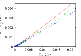
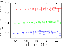
Figure 3: The leading (left) and corrections to (right) finite-size scaling for the Yang-Lee edge for the RSIM in two dimensions for weak ($p=0.88889$, upper data set, red online), moderate ($p=0.75$, middle set, green online) and strong ($p=0.66661$, lower set, blue online) dilution values.

The FSS for the lowest lying Lee-Yang zeros are plotted in Fig. 2 and the results of the corresponding fits are also listed in Table 3. The fits to the leading power-law behaviour are consistent with the theoretical value $\Delta/\nu=16/8$. Accepting this leading value, and fitting for the corrections lead to values of $\hat{\rho}$ compatible with zero. From Eq.(48), then, one can estimate $\hat{\Delta}$ using the established values of $\nu$, $\Delta$ and $\hat{\nu}-\hat{q}$. These estimates for $\hat{\Delta}$ are listed in Table 3.

Exponent	Theoretical value	$p=0.88889$	$p=0.75$	$p=0.66661$
$\gamma/\nu$	$7/4=1.75$	$1.747\pm 0.007$	$1.755\pm 0.005$	$1.752\pm 0.007$
$\Rightarrow\nu$	$1$	$1.002\pm 0.004$	$0.997\pm 0.003$	$0.999\pm 0.004$
$\hat{\zeta}=(\nu{\hat{\gamma}}-\gamma\hat{\nu}+\gamma\hat{q})/\nu$	0	$-0.01\pm 0.03$	$0.02\pm 0.03$	$0.01\pm 0.03$
$\Rightarrow\hat{\nu}-\hat{q}$	1/2	$0.51\pm 0.02$	$0.49\pm 0.02$	$0.49\pm 0.02$
$\Delta/\nu$	$15/8=1.875$	$1.879\pm 0.004$	$1.878\pm 0.006$	$1.878\pm 0.006$
$\hat{\rho}=(\nu{\hat{\Delta}}+\Delta\hat{\nu}-\Delta\hat{q})/\nu$	0	$-0.01\pm 0.02$	$0.04\pm 0.02$	$0.01\pm 0.03$
$\hat{\Delta}$	-15/16 = - 0.9375	$-0.95\pm 0.02$	$-0.95\pm 0.03$	$-0.95\pm 0.03$
$\alpha$	0	$-0.02\pm 0.03$	$0.01\pm 0.02$	$0.00\pm 0.03$
$\hat{\alpha}$	0	$-0.02\pm 0.05$	$-0.01\pm 0.03$	$-0.04\pm 0.05$

Table 3: Estimates for critical and logarithmic-correction from fits to the scaling behaviour of the susceptibility and first Lee-Yang zeros for the 2D RSIM. These estimates agree with the JSSL theoretical values.

To summarize the situation at this point, analyses of the FSS of the susceptibility and the Yang-Lee edge yield results which are dilution-independent for both the leading and logarithmic-correction exponents and fully compatible with the theoretical predictions of JSSL.

We finally turn to the density of zeros (45). For large enough lattice size, it is expected that the integrated density $G_{\infty}(r)$ may be estimated from finite lattices as KeJo06a

$$G_{L}(r_{j}(L))=\frac{2j-1}{2L^{d}}\,,$$ (51)

where $j$ is the index of the zero $r_{j}(L)$. We note that unlike the specific heat, there is no constant term contaminating the expression (45), allowing $\alpha$ and $\hat{\alpha}$ to be cleanly extracted (having already established $\Delta$ and $\hat{\Delta}$).

The density distribution function of zeros is plotted in Fig. 3 using the first four zeros for lattices from size $L=32$ to $L=256$ ($28$ points in all) for each value of the dilution. Excellent data collapse is evident in each case, and fits indicate that each curve goes through the origin, as it should at the critical value of the temperature. The potential logarithmic corrections are firstly ignored and fits to the leading scaling of the density are made. For $p=0.88889$, fits to the eight lowest data points yield and $(2-\alpha)/\Delta=1.076(16)$, corresponding to the estimate $\alpha=-0.02(3)$. The corresponding results in the $p=0.75$ and $p=0.66661$ cases are $(2-\alpha)/\Delta=1.062(10)$ ($\alpha=0.01(2)$) and $(2-\alpha)/\Delta=1.066(15)$ ($\alpha=0.00(3)$), respectively. These results for $\alpha$ are gathered in Table 3. We next accept the theoretical value $\alpha=0$ for each dilution and explore potential multiplicative logarithmic corrections by plotting $\ln G-16/15\ln r$ against $\ln{(\ln{r})}$ in Fig.3. The Ansatz (52) becomes

$$G_{\infty}(r)\sim r^{\frac{16}{15}}(\ln{r})^{\hat{\alpha}}\,.$$ (52)

A fit to all data points for $p=0.88889$ gives $\hat{\alpha}=0.012(3)$, four standard deviations from the theoretical value of zero. However, focusing on the scaling region closer to the origin establishes compatibility with the DDJ value. For example, fitting to the lowest eight data points yields $\hat{\alpha}=-0.02(5)$. The equivalent results for $p=0.75$ and $p=0.66661$ are $\hat{\alpha}=-0.01(3)$ and $-0.04(5)$, respectively. The corresponding fits are depicted in Fig. 3 and the estimates for $\hat{\alpha}$ are summarized in Table 3. These values constitute numerical evidence that $\alpha=\hat{\alpha}=0$, independent of dilution and in favour of DDJ and JSSL.

5.2 The Four-Dimensional Case

Starting with the weaker dilution value $p=0.8$, ignoring logarithmic corrections, and fitting to the leading form of (47) yields the estimate $\gamma/\nu=2.14\pm 0.01$ using lattice sizes $L=8-48$ (see Fig. 4). Attributing the deviation from the mean-field value $\gamma/\nu=2$ to the logarithmic corrections, we find an appropriate fit yields $\hat{\zeta}=0.39(3)$ for $8\leq L\leq 48$. Thus the FSS logarithmic corrections have moved from the pure value $\hat{\zeta}=0.5$ towards the theoretical estimates for the diluted value, namely $\hat{\zeta}\approx 0.25$ to $0.26$. The same analysis for the FSS of the susceptibility at the stronger dilution value $p=0.5$ gives similar results: the leading exponent is estimated at $\gamma/\nu=2.13\pm 0.02$ and the correction exponent is $\hat{\zeta}=0.37(4)$ for $8\leq L\leq 48$. These results are summarised in Table 4, together with results obtained from the same fits with the smallest lattices removed.

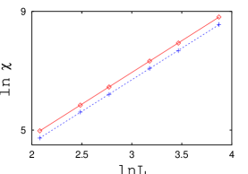
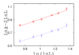
Figure 4: The leading FSS (left) and corrections (right) for the susceptibility in the RSIM in 4D for weak ($p=0.8$, upper data set, red online) and strong ($p=0.5$, lower set, blue online) dilution values.

The FSS behaviour for the Yang-Lee edge is plotted in Fig. 5. Fitting only to the leading behaviour in (48), for the weaker dilution given by $p=0.8$, one obtains $\Delta/\nu=3.055(8)$, using all lattice sizes and at the stronger dilution value $p=0.5$ we obtained $\Delta/\nu=3.068(13)$. Again, we interpret these as supportive of the Gaussian leading behaviour $\gamma/\nu=3$ with logarithmic corrections.

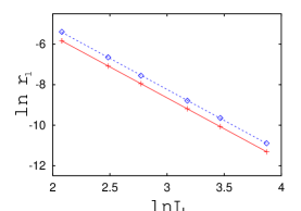
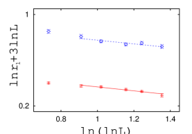
Figure 5: The leading FSS (left) and corrections (right) for the Yang-Lee edge in the RSIM in 4D for weak ($p=0.8$, lower data set, red online) and strong ($p=0.5$, upper set, blue online) dilution values.

These logarithmic-correction exponents are estimated by fitting to (48), with the various theories in the literature indicating that $\hat{\rho}=-0.125$ to $-0.13$. We find clean evidence in support of this with the estimates $\hat{\rho}=-0.15(2)$ and $\hat{\rho}=-0.20(4)$ at $p=0.8$ and $p=0.5$ respectively, using $L=8$–$48$. Dropping the smallest lattice sizes from the FSS analysis yields even more convincing results, namely $\hat{\rho}=-0.17(4)$ and $\hat{\rho}=-0.16(5)$ at weak and strong dilution, respectively. Each of these are supportive of GJ84 ; Ah76 ; Boris4D ; GeDe93 ; BaFe98 and are summarised in Table 4.

The integrated densities of zeros is calculated in a similar manner to the 2D case and are plotted in Fig. 6 for $p=0.8$ and $p=0.5$ alongside the equivalent in the pure $p=1$ case. A fit to the leading behaviour $G(r)\sim r^{(2-\alpha)/\Delta}$ yields $(2-\alpha)/\Delta=$ 1.32(3), 1.32(1) and 1.32 (1) for $p=1$, $p=0.8$, and $p=0.5$ respectively. These are compatible with the theoretical value $4/3$, independent of dilution strength. The errors are too large for us to be confident about the equivalent density analysis for the logarithmic corrections and instead we examine the specific heat directly, albeit in a rather unusual manner.

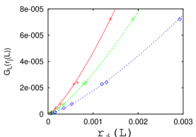
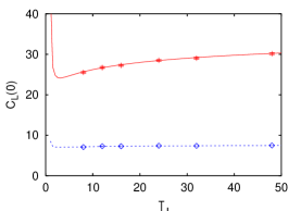
Figure 6: Left: The integrated density of zeros for the pure Ising model (upper curve, red online) and the RSIM in 4D with $p=0.8$ (middle curve, green online) and $p=0.5$ (lower curve, blue online). Right: The specific heat for $p=0.8$ (upper curve, red onlune) and for $p=0.5$ (lower curve, blue online) in the 4D RSIM.

Differentiating Ansatz (50) for the specific heat, one finds its slope vanishes when $C_{L}(0)=A$ (the asymptote $L\rightarrow\infty$) and when $L=\exp{((53/12)\hat{\alpha}^{2})}$. The specific heat is plotted for the two dilution values in Fig. 6, from which it is clear that the second occurrence of zero slope is for a lattice size smaller than $L=8$. On this basis, one may conclude $\hat{\alpha}{\rm{\raisebox{-3.22916pt}{ {\small\shortstack{$<$ \\ $\sim$}} }}}\sqrt{12/53}\sqrt{\ln{8}}\approx 0.7$, and therefore exclude the values $\hat{\alpha}\approx 1.237$ and $\hat{\alpha}\approx 1.246$ given in Boris4D ; GeDe93 . The specific-heat curves plotted in Fig. 6 are best fits to the Ansatz (50) with $\hat{\alpha}$ fixed $1/2$, the alternative value from GJ83 ; Ah76 ; BaFe98 .

$L$-range		$8-48$	$12-48$	$8-48$	$12-48$
$p$		$\hat{\zeta}$		$\hat{\rho}$
$0.8$		$0.39\pm 0.03$	$0.42\pm 0.04$	$-0.15\pm 0.02$	$-0.17\pm 0.04$
$0.5$		$0.37\pm 0.04$	$0.40\pm 0.06$	$-0.20\pm 0.04$	$-0.16\pm 0.05$

Table 4: Estimates for FSS exponents for various weak and strong dilution. One expects that $\chi_{L}\sim L^{2}(\ln{L})^{\hat{\zeta}}$ where $\hat{\zeta}\approx 0.25$ to $0.259$ and $r_{1}\sim L^{-3}(\ln{L})^{\hat{\rho}}$, where $\hat{\rho}\approx-0.125$ to $-0.130$. (In contrast, the pure $p=1$ theory is known to have $\hat{\zeta}=1/2$ and $\hat{\rho}=-1/4$.)

6 Conclusions

We have presented reviews on the quenched-disordered Ising model in two and four dimensions, where the specific-heat exponent of the pure models vanish and no clear Harris prediction for critical behaviour at the phase transitions can be made. This circumstance has resulted in both the 2D and 4D models being controversial.

In the 2D case, the debate has persisted for over thirty years. After confirming the JSSL predictions GJ83 ; Boris2D ; SL ; JuSh96 for the logarithmic corrections to scaling for the susceptibility in the random-site version of that model, we determined the Lee-Yang zeros to high accuracy and verified that their logarithmic corrections also accord with the JSSL scenario.

In the 2D model, the precise behavior of the specific heat has been especially controversial and notoriously difficult to pin down directly. Using recently developed scaling relations for logarithmic corrections KeJo06a ; KeJo06b , together with FSS and Lee-Yang zeros, we have presented an alternative approach, which strongly favours the DDJ scenario DD ; GJ83 ; GJannouncement ; GJ84 ; Boris2D ; SL ; JuSh96 . These analyses were carried out at weak, moderate and strong dilution values, thereby supporting of the strong scaling hypothesis that the exponents are dilution independent.

In the 4D case, our analysis also strengthens the analytical predictions that the Gaussian fixed point of the pure model dominates scaling and that the logarithmic corrections in the RSIM differ from those in the pure model as predicted in GJ83 ; Ah76 ; Boris4D ; GeDe93 ; BaFe98 . Furthermore, we have succeeded in discriminating between some of the detailed analytic predictions in the literature, and and our analysis favours the predictions of GJ83 ; Ah76 ; BaFe98 over those of Boris4D ; GeDe93 .

References

- (1) A.B. Harris, J. Phys. C 7, 1661 (1974).
- (2) Vik. S. Dotsenko and Vl. S. Dotsenko, JETP Lett. 33, 37 (1981); Adv. Phys. 32, 129 (1983).
- (3) M. Suzuki, Prog. Theor. Phys. 51, 1992 (1974).
- (4) G. Jug, Phys. Rev. B 27, 609 (1983); ibid 4518 (1983).
- (5) R. Folk, Yu. Holovatch and T. Yavors’kii, Uspiekhi Fizichieskikh Nauk, 173,175 (2003) [Physics-Uspiekhi, 46, (2003) 169]; P.E. Berche P.E., C. Chatelain, B. Berche and W. Janke, Eur. Phys. J. B 38, 463 (2004); D. Ivaneyko, J. Ilnytskyi, B. Berche and Yu. Holovatch, Physica A 370, 163 (2006). See also N.A. Shpot, Zh. Eksp. Teor. Fiz. 98, 1762 (1990) [Sov. Phys. JETP 71, 989 (1990)].
- (6) G. Jug, in Multicritical Phenomena, edited by R. Pynn and A. Skyeltorp, Proceedings of the 1983 Geilo School [NATO ASI held April 10-21 1983 in Geilo, Norway] (NATO ASI Series B: Physics, Vol. 106, Plenum Press, New York 1984), 329.
- (7) G. Jug, Phys. Rev. Lett. 53, 9 (1984).
- (8) B.N. Shalaev, Sov. Phys. Solid State 26, 1811 (1984); Phys. Rep. 237, 129 (1994).
- (9) R. Shankar, Phys. Rev. Lett. 58, 2466 (1987); ibid. 61, 2390 (1988); A.W.W. Ludwig, Phys. Rev. Lett. 61, 2388 (1988); Nucl. Phys. B 330, 639 (1990).
- (10) G. Jug and B.N. Shalaev, Phys. Rev. B 54, 3442 (1996).
- (11) R. Kenna, D.A. Johnston, and W. Janke, Phys. Rev. Lett. 96, 115701 (2006).
- (12) R. Kenna, D.A. Johnston, and W. Janke, Phys. Rev. Lett. 97, 155702 (2006).
- (13) S.L.S. de Queiroz, Phys. Rev. E 51, 1030 (1995).
- (14) S.L.A. de Queiroz, J. Phys. A 30, L443 (1997); J.C. Lessa and S.L.A. de Queiroz, Physical Review E 74, 021114 (2006).
- (15) F.D.A Aarão Reis, S.L.A de Queiroz and R.R. dos Santos, Phys. Rev. B 56, 6013; D. Stauffer, F.D.A. Aarão Reis, S.L.A. de Queiroz, and R.R. dos Santos, Int. J. Mod. Phys. C 8, 1209 (1997).
- (16) F.D.A. Aarão Reis, S.L.A. de Queiroz and R.R. dos Santos, Phys. Rev. B 54, R9616 (1996).
- (17) P.N. Timonin, Sov.Phys.-JETP 68, 512 (1989).
- (18) K. Ziegler, J. Phys. A 21, L661 (1988).
- (19) K. Ziegler, Nucl. Phys. B 344, 499 (1990); K. Ziegler, Europhys. Lett. 14, 415 (1991).
- (20) V.N. Plechko, Phys. Lett. A 239, 289 (1998); G. Jug has obtained the same results for the 2D RSIM (private communication and to be published).
- (21) D. Zobin, Phys. Rev. B 18, 2387 (1978).
- (22) V.B. Andreichenko, Vl. S. Dotsenko, W. Selke, and J.-S. Wang, Nucl. Phys. B 344, 531 (1990); J.-S. Wang, W. Selke, Vl. S. Dotsenko, and V.B. Andreichenko, Europhys. Lett. 11, 301 (1990) ; J.-S. Wang, W. Selke, Vl. S. Dotsenko and V.B. Andreichenko, Physica A 164, 221 (1990); A.L. Talapov and L.N. Shchur, J. Phys.: Condens. Matter 6 8295, (1994) .
- (23) A. Roder, J. Adler, and W. Janke, Phys. Rev. Lett. 80, 4697 (1998); Physica A 265, 28 (1999).
- (24) J.-K. Kim, Phys. Rev. E 62, 8798 (2000).
- (25) M. Hasenbusch, F.P. Toldin, A. Pelissetto and E. Vicari, Phys. Rev. E 78, 011110 (2008) .
- (26) H.G. Ballesteros, L.A. Fernández, V. Martín-Mayor, A. Muñoz Sudupe, G. Parisi, and J.J. Ruiz-Lorenzo, J. Phys. A 30, 8379 (1997).
- (27) W. Selke, L.N. Shchur, and O.A. Vasilyev, Physica A 259, 388 (1998).
- (28) J.-K. Kim, Phys. Rev. B 61, 1246 (2000).
- (29) H.-O. Heuer, Phys. Rev. B 45, 5691 (1992).
- (30) J.-K. Kim and A. Patrascioiu, Phys. Rev. Lett. 72, 2785 (1994); J.-K. Kim and A. Patrascioiu, Phys. Rev. Lett. 73, 3489 (1994); J.-K. Kim and A. Patrascioiu, Phys. Rev. B 49, 15764 (1994).
- (31) R. Kühn, Phys. Rev. Lett. 73, 2268 (1994); R. Kühn and G. Mazzeo, Phys. Rev. Lett. 84, 6135 (2000).
- (32) I.A. Hadjiagapiou, A. Malakis and S.S. Martinos, Physica A 387, 2256 (2008).
- (33) B. Berche and C. Chatelain, in Order, Disorder and Criticality, edited by Yu. Holovatch, World Scientific, Singapore, 2004, p. 146.
- (34) S. Wiseman and E. Domany, Phys. Rev. E 51, 3074 (1995); 52, 3469 (1995).
- (35) N.G. Fytas, A. Malakis and I.A. Hadjiagapiou, J. Stat. Mech. P11009 (2008).
- (36) W. Selke, F. Szalma, P. Lajkó and F. Iglói, J. Stat. Phys., 89, 1079 (1997); F. Iglói, P. Lajkó, W. Selke and F. Szalma and J. Phys. A, 31, 2801 (1998); F. Szalma and F. Iglói, J. Stat. Phys., 95, 763 (1999); P. Lajkó and F. Iglói, Phys. Rev. E 61, 147 (2000).
- (37) W. Selke Phys. Rev. Lett. 73, 3487 (1994).
- (38) S.L.A. de Queiroz and R.B. Stinchcombe, Phys. Rev. B 46, 6635 (1992); 50, 9976 (1994).
- (39) L.N. Shchur and O.A. Vasilyev, Phys. Rev. E 65, 016107 (2001).
- (40) J.-K. Kim, cond-mat/9502053.
- (41) M. Fähnle, T. Holey and J. Eckert. J. Mag. Magn. Mat. 104-107, 195 (1992).
- (42) K. Sawada and T. Osawa, Prog. Theor. Phys. 50, 1232 (1973) ; T. Tamaribuchi and F. Takano, ibid. 64, 1212 (1980); T. Tamaribuchi, ibid. 66, 1574 (1981).
- (43) M. Henkel and M. Pleimling, Phys. Rev. B 78, 224419 (2008).
- (44) A. Aharony, Phys. Rev. B 13, 2092 (1976).
- (45) B.N. Shalaev, Zh. Eksp. Teor. Fiz. 73, 2301 (1977) [Sov. Phys. JETP 46, 1204 (1977)].
- (46) D.J.W. Geldart and K.De’Bell, J. Stat. Phys. 73, 409 (1993).
- (47) J.J. Ruiz-Lorenzo, J. Phys. A 30, 485 (1997).
- (48) H.G. Ballesteros, L.A. Fernández, V. Martín-Mayor, A. Muñoz Sudupe, G. Parisi and J.J. Ruiz-Lorenzo, Nucl. Phys. B 512, 681 (1998).
- (49) M. Hellmund and W. Janke, Phys. Rev. B 74, 144201 (2006).
- (50) U. Wolff, Phys. Rev. Lett. 62, 361 (1989).
- (51) R. Kenna and J.J. Ruiz-Lorenzo, Phys. Rev. E 78, 031134 (2008).
- (52) A. Gordillo-Guerrero, R. Kenna and J.J. Ruiz-Lorenzo, in preparation.