The long-lived stau as a thermal relic
Technische Universität München, Physik Department, T30d
Max Planck Institut für Physik (Werner Heisenberg Institut)
Dissertation
The long-lived stau as a thermal relic
Josef Pradler
Vollständiger Abdruck der von der Fakultät für Physik der Technischen Universität München zur Erlangung des akademischen Grades eines
Doktors der Naturwissenschaften (Dr. rer. nat.)
genehmigten Dissertation.
| Vorsitzender: | Univ.-Prof. Dr. L. Oberauer | |
| Prüfer der Dissertation: | 1. | Univ.-Prof. Dr. A. Ibarra |
| 2. | Univ.-Prof. Dr. W. F. L. Hollik |
Die Dissertation wurde am 23.06.2009 bei der Technischen Universität München eingereicht und durch die Fakultät für Physik am 20.07.2009 angenommen.
Summary
The results presented in this thesis have in part already been published in Refs. [1, 2, 3, 4, 5] listed overleaf (page LABEL:publications). We consider physics beyond the Standard Model which implies the existence a of long-lived electromagnetically charged massive particle species (CHAMP) which we denote by . We discuss in detail the unique sensitivity the early Universe exhibits on the mere presence and on the decay of such a particle. A CHAMP can be realized in supersymmetric (SUSY) extensions of the Standard Model. We carry out a detailed study of gravitino () dark matter scenarios in which the lighter scalar tau (stau, ) is the lightest Standard Model superpartner so that . We also provide a thorough investigation of the thermal freeze-out process of .
The thesis is divided into three parts:
Part I: In this part we consider a generic but weak-scale CHAMP. In Chapter 1 we set the stage for the coming investigations by shortly reviewing the framework of Big Bang Nucleosynthesis (BBN), by working out the typical CHAMP freeze-out abundance, and by reviewing the stringent constraints arising from such a decaying component during/after BBN. We also take a critical look at the BBN constraints arising from the hadronic decay modes of an arbitrary exotic. In particular, we develop on a refined treatment of the Coulomb stopping mechanism of charged hadrons.
In Chapter 2 we discuss the physics which emerges when the light elements fused in BBN are captured by at the time of primordial nucleosynthesis. Since the associated, most striking effects were only discovered recently, we provide a detailed exposition of the topic. In particular, we explicitly show how to obtain the rates for bound state formation which carry a finite charge radius correction of the nucleus. In the remainder of this chapter, which is based on [4], we focus on the catalytic production of and . There, we also discuss the issue of a potential late-time catalysis due to proton-CHAMP bound states. Upon solution of the full set of Boltzmann equations we obtain stringent constraints on the primordial presence of long-lived from overproduction of . Moreover, setting an upper limit on the abundance of primordial allows us to constrain this scenario also from catalytic production.
Part II: The second part is devoted to scenarios in which is the lightest supersymmetric particle (LSP) and is the next-to-lightest SUSY particle (NLSP). In Chapter 3 we focus on the gravitino LSP as a dark matter candidate. We recollect the results on thermal gravitino production, consider explicitly the post-inflationary reheating process, and obtain an update on the upper bound on the reheating temperature of the Universe from thermal production.
In Chapter 4 we then focus on gravitino dark matter scenarios in which is the NLSP. This chapter resembles many of the results of the research papers [1, 2, 3, 4]. We constrain the gravitino-stau scenario by incorporating the BBN bounds from -decays previously obtained in the literature. In addition, the concrete realization of the long-lived CHAMP scenario allows us to employ our results on the catalytic production of and . In the framework of the constrained minimal supersymmetric Standard Model (CMSSM) a NLSP can be naturally accommodated. There, we show that the novel catalytic effects severely constrain the reheating temperature of the Universe and potentially imply very heavy superparticle mass spectra which will be hard to probe at the upcoming Large Hadron Collider (LHC) experiments. We also consider explicitly the possibility of a non-standard cosmological evolution and check for the viability of thermal leptogenesis.
Part III: Chapter 5 constitutes the final part of this thesis and is based on [5]. There, we take an in-depth look into the chemical decoupling process of the long-lived from the primordial plasma. The quantity of interest is the thermal freeze-out abundance of the stau. We identify its dependence on the crucial SUSY parameters and also show that it sensitively depends on the details of the Higgs sector. Stau annihilation into final state Higgses as well as resonant annihilation via the heavy CP even Higgs boson can substantially deplete the decoupling yield. Remarkably, we find these features are already realized in the CMSSM. In those regions of the parameter space even the most restrictive bounds from the thermal catalysis of BBN reactions can potentially be respected. We discuss the implications for the gravitino-stau scenario.
The results obtained in this thesis have in part already been published in the following references:
| [1] | Constraints on the Reheating Temperature in | ||
| Gravitino Dark Matter Scenarios | |||
| J. Pradler and F. D. Steffen | |||
| Phys. Lett. B 648, 224 (2007) [arXiv:hep-ph/0612291] | |||
| [2] | Implications of Catalyzed BBN in the CMSSM with | ||
| Gravitino Dark Matter | |||
| J. Pradler and F. D. Steffen | |||
| Phys. Lett. B 666, 181 (2008) [arXiv:0710.2213] | |||
| [3] | CBBN in the CMSSM | ||
| J. Pradler and F. D. Steffen | |||
| Eur. Phys. J. C 56, 287 (2008) [arXiv:0710.4548] | |||
| [4] | Constraints on Supersymmetric Models from Catalytic | ||
| Primordial Nucleosynthesis of Beryllium | |||
| M. Pospelov, J. Pradler, and F. D. Steffen | |||
| JCAP 0811, 020 (2008) [arXiv:0807.4287] | |||
| [5] | Thermal Relic Abundances of Long-Lived Staus | ||
| J. Pradler and F. D. Steffen | |||
| Nucl. Phys. B 809, 318 (2009) [arXiv:0808.2462] |
Acknowledgements
I would first like to express my gratitude towards my research advisor Frank Daniel Steffen at the Max Planck Institute for Physics (MPI) for his continuous support, collaboration, and for the many interesting discussions we had. I further thank him for the coordination of the International Max Planck Research School from where I also have received my funding. I am thankful to the MPI for providing an optimal place to work, in particular, to the secretary Rosita Jurgeleit for her friendly help and to Thomas Hahn for his computer support.
I would like to thank Alejandro Ibarra for being my official advisor at the Technical University Munich and thus for providing the academic framework to my PhD studies.
For his support, advice, and for holding together the enjoyable atmosphere in the MPI “Astroparticle Group” I am grateful to Georg Raffelt.
Many insights of the first part I owe to Maxim Pospelov whom I also would like to thank for his invitation to the University of Victoria. I am grateful to Gary Steigman for his friendly explanations during his visit in Munich. Simon Eidelman, Tilman Plehn and Stefan Hofmann I want thank for their general advice.
Many thanks to the friends which I had the chance to meet at the MPI, in particular, to Steve Blanchet, Koushik Dutta, Florian Hahn-Woernle, Max Huber, and Felix Rust.
For their friendship I am also most grateful to Ulrich Matt and Erik Hörtnagl.
I am deeply indebted to my family, foremost to my parents, for their unconditional love and support and to Irina Bavykina for all her understanding, encouragement, and patience over the last three years.
To the memory of Florian Kunz.
Part I BBN with a long-lived CHAMP
Chapter 1 BBN and particle decays
We start this work with a brief introduction into the framework of Big Bang Nucleosynthesis (BBN) reviewing abundance predictions of some of the primordial light elements and discussing their current observational status (Sects. 1.1 and 1.2). In Sec. 1.3 we then carry out a simplified treatment of the chemical decoupling of a long-lived CHAMP (). This frames the thermal X-abundance region and in Sec. 1.3 we shall see that with it are associated strong limits on the energy release from decays during/after BBN.
In Sec. 1.5 we investigate in some detail the stopping mechanism of injected particles short after the main stage of primordial nucleosynthesis. There, we will recover existing results of the literature but also develop on a refined treatment of Coulomb stopping of injected charged hadrons.
1.1 Primordial nucleosynthesis after WMAP
The cumulative evidence from observations of the Hubble expansion as well as of the cosmic microwave background (CMB) radiation has put the hot Big Bang model on firm footing. In addition, one of the pillars on which modern day cosmology rests on is the framework of BBN. Relying solely on Standard Model physics and a Friedmann-Robertson-Walker Universe, an overall agreement between the BBN predictions and the observationally inferred primordial abundances of the light elements , , , and is found. This is truly striking given that those elements span nine orders of magnitude in number and that light element observations are performed in vastly different astrophysical sites. It is this concordance which provides direct evidence that the Universe must once have had a temperature .
Standard BBN (SBBN) has only one free parameter, the baryon-to-photon ratio . It measures the nucleon content of the primordial plasma and controls the rates of the processes which eventually lead to the fusion of the light elements. With the measurements of the Wilkinson Microwave Anisotropy Probe (WMAP) satellite experiment [6, 7, 8] unprecedented precision data on the multipoles of the CMB angular power spectrum became available. Based on a CDM model, i.e., a flat Universe filled with baryons, cold dark matter, neutrinos, and a cosmological constant, this has allowed one to pin the baryon density down to [9] with parameterizing the Hubble constant . The value implies a baryon-to-photon ratio111This follows from the WMAP 5-year data set. For comparison, the 3-year result implied [7]. The conversion from to requires knowledge of the average mass per baryon [10]. of [9]
| (1.1) |
so that we have knowledge of the baryon content of the Universe at the time of photon decoupling to accuracy (at C.L.). Using (1.1) and/or other non-BBN determinations of as input for primordial nucleosynthesis makes BBN a parameter-free theory. When we talk about the SBBN light element predictions in the following we shall mean the outlined minimal framework of primordial nucleosynthesis with fixed by the CMB measurements.
1.2 BBN as a probe for New Physics
The comparison of SBBN predictions with the observationally inferred primordial light element abundances makes the theory of primordial nucleosynthesis a powerful tool to test and to constrain models of New Physics.
A true success of the standard cosmological model is the emerging concordance between the SBBN predicted deuterium abundance and the measurements of (in number) in hydrogen-rich clouds absorbing the light of background quasars at high redshifts. Those astrophysical sites are believed to be most appropriate to yield an estimate on the primordial fraction . Including the latest measurement [11] of this ratio, the weighted mean of seven determinations reads [12]
| (1.2) |
Conversely, with an uncertainty which is comparable to that of weak and nuclear rates used in BBN codes, the SBBN deuterium abundance can be predicted in the -range of interest as [13]
| (1.3) |
In the last expression we have used the CMB inferred baryon-to-photon ratio (1.1) and added errors in quadrature. As can be seen, both values agree within their range. Indeed, despite the difficult observations, deuterium is the baryometer of choice. Because of its weak binding energy, is only destroyed in astrophysical environments so that its post-BBN evolution is monotonic. Moreover, the SBBN prediction shows a strong sensitivity on the baryon-to-photon ratio, . Any physical process which is triggered by extending the SBBN framework must not spoil the agreement between prediction and observation.
Though the agreement in deuterium is impressive it may still only be a coincidence. Let us consider which is the most tightly bound element among the SBBN products. The primordial mass fraction is defined as222The convention to call the mass fraction is slightly misleading since with () denoting the mass of the proton (alpha-particle). However, what is observed is and it represents the abundance in mass within accuracy.
| (1.4) |
and with this makes the second most abundant element after hydrogen. The estimate in the last relation already follows from the observation that most neutrons available are finally bound in and that the neutron-to-proton ratio in number at the onset of BBN is . Observationally, is inferred from helium and hydrogen recombination lines measured by now in more than 80 extragalactic HII regions of low-metallicity. Following [13], the estimate for primordial mass fraction reads where the large adopted error reflects the fact that systematic uncertainties may well dominate; cf. [13] and references therein. Though the value is somewhat low there is currently no clear discrepancy with its SBBN prediction, the latest one reading [14]. It should be noted, however, that is a poor baryometer varying only logarithmically with . Contrariwise, being very sensitive to and thus to the Hubble rate, acts as a powerful discriminator between models predicting additional relativistic degrees of freedom at the onset of BBN.
Among the most generic ways how physics beyond the Standard Model can affect the output of BBN are, e.g., a change in timing of the reactions caused by new contributions to the Hubble expansion rate, non-thermal nuclear reactions from late decays and annihilation of heavy particles, and the thermal catalysis of nuclear reactions caused by electromagnetic or strongly interacting relics. In this regard, the stable lithium isotopes have attracted much attention because they turn out to be very sensitive on the latter two effects.
Standard BBN has a long-standing lithium problem. Let us first discuss the heavier and more stable isotope . At it is produced mainly in form of via which then beta decays via electron capture into after BBN. The cross section for the fusion also dominates the error on the SBBN prediction. With a recent update of the reaction cross section [14] the authors tighten the SBBN prediction to
| (1.5) |
Lithium is observed in absorption spectra in the atmospheres of metal-poor stars in the galactic halo as well as in stars of galactic globular clusters. A link between the measured with a primordial origin was first promoted in [15]. What has become known as the “Spite-plateau” was an observed constant lithium abundance of in halo dwarfs of low metallicity333 with the solar abundance [16]. and which corresponds to using . Ever since much work has been done and other groups found similar values so that there seems to be a clear discrepancy with the SBBN prediction (1.5) being a factor of a few too high. Indeed, the indication of a correlation of with [17, 18] tilts the plateau so when extrapolating to smallest metallicities values as low as [19] have been inferred. Moreover, such an increasing discrepancy is not alleviated by the most recent observation that the abundance in extremely metal-poor stars with is on average lower than in those (plateau) stars of higher metallicity [20].444 denotes the decimal exponent. For example, from to is . In this work we will not touch the problem. Instead, we concentrate much of our attention to the second stable lithium isotope .
The measurements of in the atmospheres of old stars of low metallicity are extremely difficult with only one firm detection in the 1990s [21, 22, 23, 24] whereas other measurements of have changed into upper limits; cf. [19] and references therein. More recently has been observed in 9 more halo dwarfs with showing a similar isotopic ratio of of [18]. This is tantalizing because it suggests the existence of a plateau mirroring the one for . At first glance, this points to a primordial origin of at the level of . However, the story is complicated by the fact that lithium is produced in galactic cosmic rays and may as well have undergone stellar depletion. Whereas in standard stellar models depletion is negligible [25, 26], is more fragile and particularly destruction in proton burning is more efficient. Indeed, non-standard models leading to lithium destruction, e.g., from inward diffusion or from rotationally induced mixing have been considered, trying to reconcile observations with its SBBN prediction; cf. [18] and references therein. However, the absence of significant scatter in the stars of the Spite-plateau demands a uniform depletion thus putting strong constraints on any of such mechanisms. When considering upper bounds on the primordial abundance many papers adopt values in the range
| (1.6) |
Comparing this with the SBBN output (see Sec. 2.4.1) this isotope shows a gaping discrepancy between prediction and observation; we refer the reader to Sec. 4.1 for a further discussion.
The lithium problem(s) has (have) particularly inspired non-standard BBN scenarios seeking their solution. Most notably in this regard are the possibility of the late-decay of a massive particle species [see Sec. 1.4] and the catalysis of nuclear reactions; see Chap. 2. In this thesis we will exclusively consider physics beyond the Standard Model with a weak-scale long-lived CHAMP which we call . We shall see that -decays as well the catalysis of nuclear reactions due to the presence of during BBN will pose strong constraints on the CHAMP abundance/lifetime parameter space.
1.3 Typical CHAMP abundances
Let us assume that the temperature of the primordial plasma was with denoting the mass of . Then, has once been tracking an equilibrium abundance. With dropping temperature, cannot maintain thermal equilibrium so that the species freezes-out.555For a low reheating temperature scenario where may not achieve thermal equilibrium see [27]. This happens approximately at the time when the rate of -annihilation drops below the Hubble expansion rate .
The key to the freeze-out abundance of lies in considering the Boltzmann equation for the total number density ,
| (1.7) |
The Hubble rate is given by
| (1.8) |
with radiation degrees of freedom and denoting the (reduced) Planck mass . The quantity is found upon a thermal average of the total annihilation cross section times the “relative velocity” ; for details on the exact definition of , , and we refer the reader to Sects. 5.2 and 1.5.1. The equilibrium number density is denoted by .
For a relic species it is customary to scale out the dilution of the number density due to the expansion of the Universe. We define the yield variable by dividing by the entropy density where is an effective degrees of freedom parameter [28]. In absence of -destroying or -producing events and as long as no entropy is released, remains constant. From (1.7) one then finds
| (1.9) |
where [28]
| (1.10) |
The exact solution of (1.9) can be rather involved and for the case where is the lighter stau, , this is presented in great detail in Part III of this thesis. Nevertheless, in order to get a feeling for the expected abundances of an electromagnetically charged relic we can employ a simplified treatment of decoupling which is based on the non-relativistic limit for .666We disregard here effects on such as coannihilation, annihilation on the threshold, or resonant annihilations [29]; see, however, Part III. In this limit, the equilibrium number density is given by
| (1.11) |
and the thermally averaged cross section may be written as [29, 30]
| (1.12) |
To find the (approximate) decoupling temperature we equate . With the notation this yields the standard result
| (1.13) |
Let us assume an annihilation cross section expanded in powers of , so that with (1.12) develops the form . Choosing on dimensional grounds777For example, the cross section for annihilation into two photons reads [31]. When considering the total abundance this gives and hence . and considering –wave annihilation, we find numerically for and . This gives the abundance at the time of chemical decoupling, . For we can neglect in (1.9) so that when accounting for residual annihilation from to one finds for the inverse of the freeze-out yield
| (1.14) |
with [32] denoting the present day photon temperature. Whenever we write in the following, is understood, i.e., the yield of the species it would have had today had it not decayed.
Taking into the account the temperature dependence of by interpolating the tabulated values in [33] and integrating (1.14) yields the following estimate on the abundance
| (1.15) |
with an approximate linear scaling in . Note that an increase in contributes linearly to , provided . Therefore, we have indicated that in (1.15) is a value more towards the upper end, corresponding to a guaranteed annihilation cross section of electromagnetic strength. A stronger coupling will allow to stay longer in equilibrium, thus receiving an additional Boltzmann suppression.
Conversely, we can constrain from below by assuming the maximum cross section of mutual annihilation which is given by the unitarity limit [34], (-wave); denotes the de Broglie wavelength of the relative motion. Using together with the reduced mass one finds with (1.12)
| (1.16) |
Employing this cross section yields an estimate on the smallest possible freeze out abundance for a weak scale electromagnetically charged relic. Using gives and
| (1.17) |
Let us see how this lower limit on the decoupling yield compares with experimental bounds on charged cosmological relics from (negative) searches of anomalous heavy isotopes of ordinary nuclei. For example, in [35] severe limits on the concentration of in form of heavy hydrogen as well as in low –nuclei have been obtained for a weak scale relic in the mass range . It was found that present day abundances in excess of
| (1.18) |
are firmly excluded.888We have obtained the constraint from the right end of the 14C-line in Fig. 7 of [35] and changed the normalization of from baryon number to entropy. For a recent compilation of other such limits along with a thorough investigation of the decoupling yield of a generic electromagnetically- or color-charged particle species confer [36]. Note that individual limits on either or exist for masses ranging from a few to multi- and they can be stronger than (1.18) by more than ten orders of magnitude; cf. [32]. Comparing (1.17) with (1.18) forces us to conclude that, under our assumption of a standard cosmological evolution, cannot be stable. Considering a charged thermal relic of finite lifetime with abundances in the range (1.17) to (1.15) sets the stage for our further investigations.
In the next chapter we shall also quantify the abundance normalized to baryon number instead of entropy. We define
| (1.19) |
where is the photon number density with denoting the Riemann Zeta function. We have chosen this notation in order to clearly distinguish the two different normalizations and it will be clear from the context whether denotes the particle itself or its abundance. The previous estimates (1.15) and (1.17) then translate into
| (1.20) |
It is also instructive to compare the abundance with that of . This will be of some importance in the discussion of catalytic BBN effects where bound states of with play a key role. Since to a very good approximation it follows from (1.4) that
| (1.21) |
we see from (1.20) that we can expect that the number density of is typically smaller than that of unless is rather heavy; here, but in concrete particle physics models with annihilating via a number of channels, a heavier is required. Indeed, when focusing on the particle content of the minimal supersymmetric Standard Model (MSSM) (plus a gravitino LSP) with , the -abundance is determined by the standard chemical decoupling and holds unless ; see Sec. 4.1.
1.4 Particle decays during BBN
Using primordial nucleosynthesis as a consistency check for the existence of long-lived particles has a long-standing history.999In this section stands for an arbitrary, not necessarily electromagnetically charged, long-lived species. When exotics decay during or after BBN electromagnetic and/or hadronic energy is injected into the plasma. Depending on timing, energy deposition, and abundance of the decaying species, the light element output can be affected significantly. The comparison with the observational bounds yields constraints on the parameter space of . From early works, e.g., [37, 38], to elaborate studies [39, 40, 41] this is still an active field of research of continuing refinement and increasing sophistication; for a most recent work see, e.g, [42]. Since we will also make use of BBN constraints on electromagnetic and hadronic energy release, we provide here a cursory overview pointing out important features. For a more detailed exposition of the topic we refer the reader to [39, 40, 41] and references therein.
- Electromagnetic constraints
-
The emerging constraints can be classified with respect to the decay mode of the exotic particle. When decays radiatively into primary high-energy photon(s) and/or electrons (charged leptons) an electromagnetic cascade is induced. The important processes are pair creation ), photon–photon scattering , Compton scattering , inverse Compton scattering , and pair creation on nuclei . The subscript ’bg’ denotes the particles which are in equilibrium with the plasma. Since the scattering on background photons is very frequent. This leads to an efficient thermalization of the cascade so that destruction of light elements does not happen frequently. However, once energetic photons are degraded below [43] they loose their ability to pair create on . The soft photons of the associated ’break-out’ spectrum are then capable to efficiently destroy those light elements whose binding energy lies below the threshold of electron pair creation. For ( [44]) this happens at whereas ( [44]) is destroyed when the photon temperature drops below . This corresponds to respective cosmic times of and when thermal nucleosynthesis reactions have long frozen out.
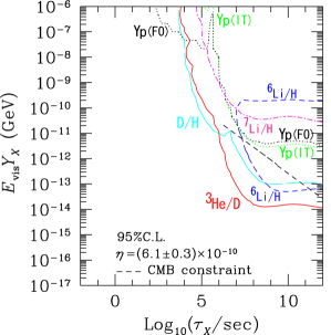
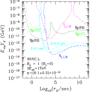
Figure 1.1: Constraints on the electromagnetic (left figure) and hadronic (right figure) energy release from -decays for ; the figures are taken from [41]. The lines represent upper limits on the quantity , i.e., on the “visible energy” released per decay times their abundance prior to decay, , and are plotted as a function of ; see main text for discussion. Constraints on the electromagnetic energy release for are shown in the left Fig. 1.1 which is taken from [41]. The lines represent upper limits on the quantity , i.e., on the “visible energy” released per decay times their abundance prior to decay, , and are plotted as a function of . Two dominant constraints are visible. For the most restrictive constraint, labeled , arises from the destruction of deuterium below its observationally inferred primordial level. For larger , however, gets dissociated and (along with and ) is also created. Since the -target is very abundant, is indeed overproduced for . Moreover, the combination is then always produced yielding the most stringent constraint on electromagnetic energy release for .
- Hadronic Constraints
-
A second class of constraints on decaying during/after BBN comes from hadronic energy release into the plasma. For example, even if dominantly decays into photons, a non-vanishing hadronic branching ratio is expected from the conversion of a (virtual) photon into a quark-antiquark pair or from charged meson production on background photons (if kinematically allowed). The partons emitted in the decay are quickly hadronized and the highly energetic fragmentation products such as protons (), neutrons (), as well as their antiparticles are released. Also long-lived mesons, namely, charged pions and kaons (), with lifetimes have a chance to interact with background nuclei before decaying. Once an energetic hadron scatters on a background nucleus, essentially or , a hadronic shower is induced. In particular, may be destroyed with secondaries further participating in interactions with the plasma constituents.
The energetic charged hadrons are downgraded in energy via electromagnetic interactions, most importantly, by Coulomb scattering , Compton scattering , and Bethe-Heitler scattering . Injected neutrons loose their energy mainly by their magnetic-moment interaction with . It is clear that emergent constraints on the hadronic energy release will sensitively depend on the competition between the rate for hadronic scattering and the rates for (electromagnetic) thermalization and/or decay (of unstable particles). Moreover, even after hadrons are stopped they may still induce neutron-to-proton interconversion processes [37].
In the right Fig. 1.1 which is taken from [41] the constraints on due to hadro-dissociation as well as - interconversion are shown for a particle with and hadronic branching ratio . The effects from photo-dissociation are not included. Note that this is an unrealistic situation since the hadron stopping process itself as well as meson decays induce electromagnetic showers. For , i.e., for , the emitted hadrons essentially deposit all their kinetic energy electromagnetically before interacting with the background nuclei. However, interconversion processes which always lead to an increase of enhances the output. The associated constraints from overproduction for two different observationally adopted limits on the primordial mass fraction are shown by the dotted lines labeled . For larger lifetimes, (), mesons typically decay before interacting hadronically. However, the stopping power for protons and neutrons rapidly decreases with dropping temperature so that is destined for being destroyed. This yields the stringent constraint on hadronic energy release for . Moreover, a small fraction of the energetic spallation products and can scatter again on ambient producing [45] (and ). This non-thermally induced fusion reaction gives the hadronic constraint labeled in Fig. 1.1. Since is efficiently destroyed in (thermal) proton burning for temperatures the constraint becomes the dominant one only for [46].
So far, the discussion has been completely generic with our ignorance on the nature of parameterized by . Constraining the particle’s parameter space requires the specification of the couplings of to Standard Model particles as well as its mass . This allows for the determination of the decay modes of along with the computation of the associated average electromagnetic and hadronic energy released per decay. Moreover, the freeze-out abundance can be calculated so that plots like in Fig. 1.1 can be employed to constrain the model. In part II of the thesis we incorporate the most stringent of the constraints for the case of a decaying stau in the gravitino dark matter scenario. There, we also provide more details as soon the problem of inclusion of such constraints becomes acute.
1.5 A critical look at hadronic constraints for
In the previous section we have noted that for () the BBN constraints on hadronic energy release sensitively depend on the competition between the hadronic and electromagnetic scattering rate (and potentially the lifetime). If injected nucleons as well as their secondaries—either produced in spallation reactions or “up-scattered” in elastic scatterings—are predominantly thermalized by interactions on background nucleons or nuclei, those constraints become stringent. Underestimating the stopping power due to electromagnetic interactions would lead to overly restrictive bounds on the hadronic energy release.
For example, in the last section we have seen that the non-thermal production of due to the energetic spallation debris and of destroyed yields the dominant hadronic constraint for . The reactions involved are and [45]. For , i.e., for , inverse Compton scattering on background photons cannot prevent low-energy hadronic interactions [37] above the lithium formation threshold . The dominant electromagnetic degradation mechanism is then Coulomb scattering. However, the rapidly diminishing number of background electrons (positrons) with dropping temperature also renders the energy loss by Coulomb scattering increasingly inefficient. Furthermore, in [40] it is claimed that the non-thermal output is boosted by a factor of ten because of a peculiarity in the Coulomb process: Once the velocity of the energetic mass-three nuclei drops below the thermal electron velocity , the stopping power seems to be strongly suppressed. This observation was first made in [37].
In light of these comments a critical look on the Coulomb stopping process is warranted. We shall pay particular attention to the velocity dependence of the cross sections, i.e., on and . In Sec. 1.5.1 (and partly also in Sec. 1.5.2) results from the literature are reconciled. In Sec. 1.5.3 we focus on the stopping of charged hadrons and incorporate the proper screening-prescription of the Coulomb interaction. In Sec. 1.5.4 we discuss the obtained results.
1.5.1 Energy transfer in binary collisions
A thorough investigation of the electromagnetic stopping of hadrons in the context of primordial nucleosynthesis has first been presented in [37]. Indeed, the treatments in [47, 41] (see Fig. 1.1) employ the results of that work. Since the stopping power sensitively depends on the velocities of the incident hadron and the target particles, we first reconcile the general result on the energy transfer obtained in [37]. Though we encounter minor disagreements they turn out to be without relevance.
Our starting point is the rate of energy loss due to binary scatterings (A1) of Ref. [37]
| (1.22) |
where denotes the energy transfer between the incident hadron and a (background) particle species with three-momentum and internal degrees of freedom. The transfer is weighted by the center-of-mass (CM) cross section and averaged over inital and final state distribution functions and , respectively. A subtle point is the appearance of the Møller velocity [28]
| (1.23) |
which is the relativistic generalization of the conventional relative velocity . The respective velocities of the hadron and the target are given by and and denotes the Flux-factor. Only in the CM frame or in the rest frame of one of the incoming particles coincides with . We stress that and denote the respective four-momenta of the energetic nucleus and of the ambient target particle in the rest frame of the thermal bath. In that frame, and when is in thermal equilibrium, the distribution functions take on their familiar form: . The upper signs in (1.22) and in the last expression refer to fermions, the lower to bosons. Finally, is the energy of the target after scattering and () is the mass of the target (indicent nucleus).
The energy transfer can be obtained by a series of Lorentz transformations: Since the scattering is elastic, in the CM frame we have . Thus, we can obtain by a Lorentz transformation of into the CM frame followed by an inverse transformation of back. is broken up as follows:101010The explicit forms of , , and are given in the Appendix 1.A at the end of this chapter. We choose to lie along the -axis and to have an angle with -plane
| (1.24) |
so that corresponds to a “head-on-head” collision. Boosting into the rest frame of the incident nucleus gives
| (1.25) |
where . Under Lorentz transformations the Møller velocity changes as [28]
| (1.26) |
which can be used to obtain the velocity of the ambient target in the rest frame of the incident particle. Confirming the expression given in [37] it reads
| (1.27) |
By the same token, the expression for the angle between and the -axis reads
| (1.28) |
which differs by a sign from [37]. Instead of explicitly carrying out the rotation which makes parallel to the -axis ( is lengthy) we use our knowledge on the form of : since . Boosting into the CM frame using one finds
| (1.29) |
where is obtained from ; . We find
| (1.30) |
In the CM frame, the scattered target three-momentum has a scattering angle with and both momenta span a plane with azimuthal angle . Thus, is given by
| (1.31) |
and with we can transform back into the rest frame of the thermal bath. This yields for the energy of the scattered background particle
| (1.32) |
from which is obtained. We encounter some sign-differences and a different angular dependence on in the last line with (A2) of [37]. This may be due to a different definition of the coordinate system and turns out to yield the same results. Since the target medium is unpolarized, is independent of and the integration over the azimuthal angles in (1.22) can be performed upon which the last line of (1.5.1) drops out. Neglecting the Fermi blocking/Bose enhancement factors in (1.22) we find (adopting the notation of [37]),
| (1.33) | ||||
| (1.34) | ||||
| (1.35) |
1.5.2 Hadron-electron scattering
Let us now focus on “Coulomb scattering” between an incident hadron and background electrons (positrons) and compute for . Note that also neutral hadrons scatter on via their magnetic moment interaction.
For spin- hadrons such as nucleons or and nuclei the hadron-photon vertex can be written as [48] with and denoting the (outgoing) four-momentum of the nucleus. The respective electric and magnetic form factors and depend on the (squared) four-momentum transfer and are normalized such that is the charge in units of and that is the magnetic moment in units of of the hadron.111111The Sachs form factors and are convenient because no interference terms appear in the cross section (1.5.2); they are related to the Dirac and Pauli form factors and via and [49]. With the definitions for and and for , in the laboratory frame, the Rosenbluth formula [50] follows from (1.5.2). The (unpolarized) differential cross section for electron-hadron scattering is readily obtained. In accordance with [48] (typo in [37]) it reads using the Mandelstam variables , and
| (1.36) |
Owing to a different vertex structure for spin-0 hadrons such as pions or , , where is the electromagnetic form factor (), one readily obtains [48]
| (1.37) |
We can expand (1.5.2) and (1.37) in terms of (typo in [37]). The expansion is most likely to fail for scattering of (light) ultra-relativistic nuclei at high temperatures of the thermal bath. To see the validity of the expansion consider the typical energy of an electron by using Maxwell-Boltzmann statistics:
| (1.38) |
Here, is the modified Bessel function of the first/second kind. For example, with , a kinetic energy of the nucleus, and one finds . Thus for the cases of interest the expansion in is fine. Since the cross-sections are independent of the azimuthal angle121212An overall sign has been dropped since it can be fixed by the integration borders.
| (1.39) |
where . Neglecting it follows
so that we find for the CM cross section for charged spin-1/2 and spin-0 nuclei
| (1.40) |
Note that we have made the approximation assuming small . Let us see if this is justified. The maximum energy transfer is realized in a back-to-back collision in the CM frame for which . Considering the case that , i.e., the case when the electron is a stationary target, it follows from (1.39) that . For example, for a proton with this gives for which is practically unchanged from unity [51]. Moreover, note that setting usually leads to an overestimation of the cross section with and decreasing for increasing [51, 52]. Consequently, the stopping power is overestimated leading to more conservative BBN constraints. For neutral hadrons we find131313For example, [32] for the neutron, being entirely anomalous.
| (1.41) |
We disagree in (1.40) and (1.41) with [37] by a factor of in the denominator. The disagreement arises as follows: Eq. (A5a) of [37] is actually Eq. (139.5) of [48]. In order to arrive at the latter equation has been used ( in the notation of [48]). However, it is more accurate to use ; recall that is the velocity of the electron as seen from the rest frame of the nucleus. We note in passing that up to corrections one has , , , and .
We can use the above expansion in to simplify in (1.5.1) for the limiting cases of ultra-relativistic and non-relativistic hadrons traversing the background plasma. Considering , i.e., an ultra-relativistic incident particle, and therefore , , and we get to leading order
| (1.42) |
Conversely, for and therefore , , and we find
| (1.43) |
Both expressions agree with the ones obtained in [37] with differing signs in (1.5.1) being compensated.
1.5.3 Cutoff considerations for charged particles
After having obtained the cross section for Coulomb and magnetic moment scattering for hadrons on electrons we make the following observation for charged particles: Though the energy transfer in a collision is smallest in the forward direction [as can be seen by the factor in Eqs. (1.42) and (1.43)], the divergence in the cross section for charged hadrons (1.40)—arising from the long-range nature of the Coulomb interaction—is too strong to be canceled. In this sense, the energy loss due to scatterings in the forward direction gives the most efficient contribution. Cutting off the angular integration in (1.34) at leads to the well known logarithmic dependence on . Of course, has to be motivated.
In a plasma, i.e., in a gas of charged particles, correlation effects lead to the screening of the long-range Coulomb interaction. In Ref. [41] the authors determine the cutoff by comparing the energy transfer to the electron with the plasma frequency
| (1.44) |
where denotes the total electronic density
| (1.45) |
In the first line we have neglected the electron chemical potential and in the second line we have imposed charge neutrality of the Universe. The upper relation in (1.45) is derived by using Maxwell-Boltzmann statistics. For , i.e., for ultra-relativistic electrons/positrons, this implies an error by a factor of . Note also that electrons freeze out in the temperature region of interest, .
The plasma frequency does, however, not provide the correct scale [53]. The screening of the electric field is a longitudinal phenomenon whereas the notion of the plasma frequency as an effective photon mass is associated with transverse plasma excitations. Electrons as well as the (ionized) light elements contribute to the screening with a scale [54]
| (1.46) |
where denotes the Debye scale with Debye length ; denotes the number density of nuclei with charge number . Note that and can be very different with . However, in the temperature region of main interest and are within a factor of a few. Moreover, since the screening scale will enter only logarithmically we neglect the contribution of the ions (in particular protons) in the following and set .
We shall distinguish two cases: For the electrons can be viewed as a stationary target. Thus, we follow the screening prescription obtained in [53] and replace (1.5.2) via
| (1.47) |
(for elastic scattering in the CM frame ) whereas for electrons have time to rearrange so that the scattering resembles one on a Yukawa-like charge distribution with screening length . Then the correct prescription reads
| (1.48) |
Given the above considerations we replace the scattering cross section (1.40) for charged particles employing the screening prescriptions (1.47) and (1.48) for the respective cases and . We find
| (1.49) |
| (1.50) |
with
| (1.51) |
In the region where acts as a regulator, i.e., for , we make the immediate observation that
For scattering in the forward direction the screening prescriptions will yield a numerical difference only for . For our cases of interest is usually a very small quantity, e.g., for or for . Thereby, only in a very small integration regime over both cross sections will be significantly different—though the integrand is largest in this area.
In order to decide which cross section is applicable for a given value of the hadron velocity , it has to be compared with the average electron/positron velocity
| (1.52) |
which is obtained by using Maxwell-Boltzmann statistics; for the formula reduces to the standard result . Note that is related to the kinetic energy of the incident hadron via . Thus, for example, a proton with has so that drops below for .
1.5.4 Discussion on Coulomb stopping
In this section we discuss in some detail the results on the energy loss for charged particles due to Coulomb interactions with the background electrons (positrons). We will also compare with a treatment found in the literature.
To see the net effect of the different screening prescriptions on the stopping power we perform a full numerical integration of (1.34) and (1.33) using the Vegas algorithm [55]. For the integration over the electron (positron) velocity knowledge of the distribution function is required. Though electrons are frozen out for they remain tightly coupled to the photon bath via Thomson scattering. This ensures that electrons maintain kinetic equilibrium so that we can make the approximation
| (1.53) |
where denotes the photon temperature. For we use , i.e., we resort to Maxwell-Boltzmann statistics in the non-relativistic limit.141414It is shown in [56] that satisfies the Boltzmann equation in the non-relativistic limit with an elastic collision term due to Thomson scattering; by comparison with (1.45). Defining the temperature of a non-relativistic particle species with arbitrary distribution as [56] it is found that the electron temperature tracks well until recombination, . There, [57]. From the definition we reproduce the second line of (1.45) by using in the form of (1.11) with ; for the case we use .
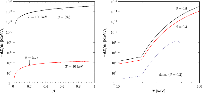
In Fig. 1.2 we show the stopping power for an injected proton computed by numerical integration from (1.33) using the different screening prescriptions. Solid lines correspond to (1.49) and dotted lines (hardly visible) are associated with (1.50). In the left panel we show in units of as a function of the proton velocity at temperatures and as labeled. In addition, the points indicate which screening prescription should be used. In the right panel we show as a function of for a relativistic proton () and a non-relativistic proton ().
From Fig. 1.2 we can make a number of observations. An immediate one is that the stopping power is essentially insensitive to the employed screening prescription. Concretely, we find that both prescriptions yield a difference in by no more than for the considered temperature range. From the right panel we see that once the velocity of the incident particle drops below the average electron velocity, the stopping power starts to decrease rapidly. This confirms the observation made in [37] and it is also intuitive since it becomes increasingly difficult to transfer momentum to the—on average—faster electrons. Indeed, for the charged hadron can even gain energy in a collision which is indicated by a sign-flip of [Eq. (1.34)] in the collinear region where (’head-on-back collision’). From the left panel we realize that the stopping power rapidly decreases with dropping temperature. This is because for the number density of electrons and positrons is Boltzmann suppressed. For the decrease is weaker because the remaining electrons fail to track their exponentially decreasing equilibrium abundance. More precisely, scales like for such low temperatures because and during radiation domination.
So far, we have only considered (screened) binary collisions of a fast charged particle traversing a QED plasma. Such a treatment gives an accurate description for those scattering events of the particle with largest energy transfers, i.e., with smallest impact parameters . Considering , the nucleus scatters simultaneously on many electrons. (Note that in our case the Debye length is much larger than the typical inter-particle distance, .) A sweeping external charge, i.e., a perturbation , induces a macroscopic electric field in the medium which acts back on the particle. The resulting energy loss per unit path length can be found by computing the work done on the particle. It equals the force exerted onto the charged hadron in direction opposite to its motion
| (1.54) |
where is a unit vector in direction. The electric field can be found by considering the macroscopic Maxwell equations with dielectric permittivity . In the non-relativistic limit and using151515Here, and () are the frequency and wave vector of the Fourier transformed fields and the expression is the limiting case for ; see [58]. for a Maxwellian plasma, the stopping power reads [59]
| (1.55) |
As can be seen by the dashed line in the left Fig. 1.2 the contribution due to the ’density effect’ is subleading. Note that the formula was derived under the premise that the velocity of the massive particle is large compared to the thermal speed of the electrons. Indeed, the argument of the logarithm in (1.55) is greater than unity only for so that the line is cut-off for . We remark that a full relativistic treatment of the energy loss of a massive particle due to the dielectric response of the medium for arbitrary velocities is complex but will not affect significantly the above made conclusions; we refer the reader to Landau’s treatment in [58].161616The case of a hot QED plasma with has been treated within the framework of thermal field theory in [60].
We can compare the full numerical integration of (1.33) with the treatment of Coulomb stopping presented in [41]. The authors employ the results of [37] which also we have taken as a starting point. Full numerical integration of (1.33) is not feasible when scanning the parameter space so that analytical approximations based on (1.42) and (1.43) have been used in [41]. Since we have observed that the employed screening prescription affects only marginally for and that and —entering the stopping power logarithmically—are not too different, it is not surprising that we find overall agreement with [41] on the energy degradation rate within a factor of a few.
We remark that obtaining constraints on the hadronic energy release of decaying involves a fair amount of modelling and computation. After calculation of the hadronic branching ratio in the decay of , each step involves uncertainties and approximations: Employing a hadronization algorithm, computing the initial energy spectra of secondaries, following the energy degradation and cascade formation due to electromagnetic and hadronic processes, and finally obtaining the yields of non-thermally produced light elements. We have seen that already the seemlingly elementary process of Coulomb stopping can become involved—especially when it is necessary to apply it to a large range of incident particle energies and plasma temperatures. In the light of these comments we close this chapter by noting that we have not found a radically different picture than that of previous considerations which would strongly influence on the strength of the hadronic constraints presented in Fig. 1.1.
Appendix 1.A Lorentz transformations
The explicit matrices for the Lorentz transformations performed in 1.5.1 are given below. The matrix describes an (active) rotation in counter-clockwise direction around the -axis when looking towards the origin. The inverse transformations , , and are obtained by the replacement , , and in , , and , respectively.
| (1.56) | ||||
| (1.57) |
Chapter 2 Bound states and catalysis of BBN
In this Chapter we now discuss (some of) the rich physics which emerges when the light elements are captured by during/after the time of primordial nucleosynthesis. We start in Sec. 2.1 by reviewing the basic properties of such bound states. Section 2.2 is devoted to the calculation of the wave functions associated with the CHAMP-nucleus system. This allows us in Sec. 2.3 to obtain recombination cross sections carrying a finite nuclear charge radius correction. The detailed exposition in Sects. 2.2 and 2.3 is of some value since (apart from exceptions) those rates are not publicly available in the literature.
In Sec. 2.4 we then consider the catalysis of BBN reactions. After a general review we employ the results from the literature on the catalyzed production of and and show explicitly how to incorporate them into a Boltzmann network calculation. In Sec. 2.5 we discuss the potential impact of neutral proton-CHAMP bound states on the synthesized elements. We close this chapter with Sec. 2.6 in which we first infer an upper limit on primordial and then present the results of our CBBN calculation which heavily constrains the -abundance/lifetime parameter space.
2.1 Basic bound state properties
The presence of negatively charged massive particles during/after primordial nucleosynthesis leads to the formation of bound states with the ionized nuclei of the light elements. In this section we shall describe the basic properties of such bound states.
In order to obtain a first estimate on the physical properties one can immediately apply the standard formulæ for the quantum mechanical motion in a Coulomb field. The characteristic size of the system is given by the Bohr radius of the system,
| (2.1) |
where and are the atomic mass and charge number of the nucleus, respectively. In the second relation we have used that the reduced mass
| (2.2) |
is given to good accuracy by the mass of nucleus, (), and that roughly where [32] is the proton mass. The binding energies of a point-like nucleus orbiting are given by the well-known formula
| (2.3) |
where denotes the principal quantum number.
For the case of a proton bound state so that the system is a factor of smaller than a hydrogen atom. Nevertheless, the – distance is still large when compared to the rms charge radius of the proton, [61]. The situation changes for heavier nuclei. For example, considering , one finds that whereas the measured rms charge radius reads [61]. Thus, we expect corrections to the naïve Bohr-like binding energies (2.3) once the finite size of the nucleus is taken into account.
In order to obtain more realistic values for the ground state energy, we need to make an assumption on the charge distribution of the nucleus. A compilation thereof is presented in [62]. We employ the Gaussian with radial coordinate from which the potential
| (2.4) |
is obtained upon solution of Poisson’s equation111We use Heaviside-Lorentz units with . . Requiring relates the parameter to the rms charge radius; . The error function is defined by .
| bound state | ||||||
|---|---|---|---|---|---|---|
| 938 | 0.88 | 28.8 | -25 | -25 | ||
| 1876 | 2.14 | 14.4 | -50 | -49 | ||
| 3727 | 1.67 | 3.6 | -397 | -347 | ||
| 5601 | 2.54 | 1.6 | -1342 | -797 | ||
| 8393 | 2.52 | 0.8 | -3575 | -1469 | ||
| † Nuclear masses are obtained from atomic masses by subtracting and correcting for the total binding energy of all electrons where we follow the prescription given in [44]. | ||||||
The above choice of the charge distribution is particularly convenient because the electric potential (2.4) is given in analytical form (2.4). This makes an application of the Rayleigh-Ritz variational method straightforward. Using the (unnormalized) trial wave function
| (2.5) |
with variational parameters and an upper bound on the true ground state energy can be obtained by minimizing the right hand side of
| (2.6) |
For the Hamiltonian of the system we use , i.e., we take .
The results of minimization of (2.6) for selected light elements along with some other basic quantities are summarized in Table 2.1. Note that the Bohr radii of bound states with elements heavier than lie within the nuclear radii. Thereby, the true binding energy for those systems is significantly reduced in magnitude as can be seen by comparing with . We remark that the binding energy is an important quantity since it directly influences on the bound state fraction of the light nuclei.
2.2 Wave functions of the relative motion
For the calculation of photo-dissociation and recombination cross sections which include the finite charge radius correction, we are in need of the actual wave functions of the – system. In the following we shall therefore obtain the wave functions for the () bound states as well as for the – continuum. It will also allow us to see how well our variationally obtained upper bounds fit the actual value of the true ground-state energy .
The Schrödinger equation for the radial part of the wave function of the relative motion is given by
| (2.7) |
As usual, denotes the spherical harmonic with orbital and magnetic quantum numbers and . For the potential we make the following choices
| (2.11) |
where “point” stands for the Coulomb potential of a point-like nucleus, “gauss” for a Gaussian charge distribution with defined in (2.4), and “h.sph” for a potential of a homogeneously charged sphere of squared radius [62]. For , is to be continued by .
2.2.1 Discrete spectrum
We solve (2.7) for and the various choices of V [Eq. (2.11)] numerically. For fixed we exploit the fact that the radial function and thus vanishes times; is the radial quantum number. The solution of (2.7) is fixed by imposing the standard boundary conditions and with and normalizing to unity, .
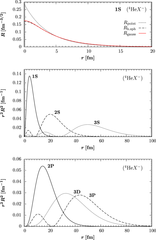
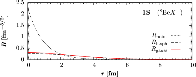
At the top of Fig. 2.1 we show the numerical solutions of the normalized radial wave function for the ground state (1S in the usual spectral notation) for the different choices (2.11) of the potential. An attenuation of the wave functions with finite charge radius relative to the Coulomb case can be seen at small . At large radii, the wave functions are Coulomb-like.222Of course, the Coulomb solution is simply given by It can further be seen that for all , i.e., the radial wave function for is rather insensitive to the concrete choice of the charge distribution. In the middle and at the bottom of Fig. 2.1 we plot , i.e., the probability density of the – distance, for and Gaussian charge distribution. Except for small radii, the curves essentially resemble distributions obtained with Coulomb wave functions. This is particularly true for the higher states as the wave functions are pushed outwards due to the centrifugal term in (2.7).
| , | ||||||
|---|---|---|---|---|---|---|
| State | ||||||
| 1S | 397 | (383) | 348 | (338) | 1.7 | 2.0 |
| 2S | 99 | (96) | 93 | (90) | 6.4 | 6.9 |
| 2P | 99 | (96) | 99 | (96) | 5.0 | 5.5 |
| 3S | 44 | (43) | 42 | (41) | 14.1 | 15.0 |
| 3P | 44 | (43) | 44 | (43) | 12.5 | 13.4 |
| 3D | 44 | (43) | 44 | (43) | 10.5 | 11.2 |
In Table 2.2 the spectrum for the cases “point” and “gauss” [Eq. (2.11)] is given for the states plotted in Fig. 2.1. In addition, also the expectation value as well as the rms radius are given for the “gauss” case in units of . We solve the Schrödinger equation (2.7) for , i.e., for , as well as for (bracketed values) in order to study the influence of a finite mass on the binding energies. The table shows that for this leads to a shift of for the ground state energy but the correction quickly becomes marginal for the states. The same is true when comparing the spectra for the different potentials. Whereas the correction to the ground state energy is substantial, , the higher states for the system essentially coincide. It is, however, interesting to note that the Coulomb degeneracy is broken. We refrain from showing the energies for the case “h.sph” since they are the same as for the “gauss” case (except for where a shift is found.) One can also see that the variational determination of the ground state energy in section 2.1 gave an accurate result.
| , | ||||||||
|---|---|---|---|---|---|---|---|---|
| State | ||||||||
| 1S | 3176 | (2956) | 1118 | (1092) | 1168 | (1138) | 3.8 | 4.2 |
| 2S | 794 | (739) | 458 | (437) | 475 | (453) | 9.8 | 10.6 |
| 2P | 794 | (739) | 652 | (620) | 650 | (618) | 6.4 | 6.9 |
| 3S | 353 | (328) | 243 | (230) | 249 | (236) | 19.0 | 20.2 |
| 3P | 353 | (328) | 306 | (290) | 307 | (290) | 14.5 | 15.5 |
| 3D | 353 | (328) | 348 | (325) | 346 | (323) | 10.9 | 11.6 |
For bound states of with heavier nuclei than , i.e., for more compact systems, we expect a pronounced behaviour of the observed effects above. Analogously to the case we can analyze . This is an interesting system because free is unstable by and decays into two alpha particles: . Indeed, the stable system is part of a CBBN reaction chain which can open the path to primordial production of [63]; see Sec. 2.4. Since the lifetime of is no experimental data on the charge radius of the isotope is available. In this section we follow [64] and adopt the value which is based on a microscopic model calculation [65]. Again, in Fig. 2.2 we plot the 1S radial solutions of the Schrödinger equation (2.7) for the various potentials (2.11). The difference between and () is now substantial. Moreover, also a slight difference between and is observable for smaller radii. We therefore expect a dependence of the ground state energy on the adopted charge distribution.
In Table 2.3 we provide the complete spectrum for with . Expectation values as well as the rms radius are also computed for the “gauss” case in units of ; . Again, we compare the energy eigenvalues for with the ones for (bracketed values). As can be seen, all states now receive substantial corrections to the Coulomb values. Moreover, we observe a shift in the 1S energy when changing the charge distribution from Gaussian to square well (in ).
Finally, we have checked all variationally determined ground state binding energies presented in Table 2.1 of the last section by explicit computation of the wave function. We find that all given in Table 2.1 are within of the numerically obtained result. Noteworthy may be the shift for . Of course, not only the assumed distribution of charge influences on but also the error on the measured or theoretically predicted charge radius is a source of uncertainty. This is of pronounced importance for the heavier nuclei because the bound state system is more compact. For our purposes, however, it is not essential to pursue this issue further; see Sec. 2.4.2 for another comment in the context of catalyzed production. In the following, we employ the binding energies determined from the Gaussian charge distribution.
2.2.2 Continuous spectrum
We are also in need of solutions of the Schrödinger equation (2.7) for if we want to obtain charge-radius corrected bound-state formation cross sections. The normalization of a numerically obtained solution is more involved since the wave functions of the –-continuum are not bounded spatially. However, a finite charge radius leads to a modification of the Coulomb form of the potential only in the vicinity of the origin. Therefore, we can take the following approach: For the solution of (2.7) has to be a linear combination of the regular and irregular Coulomb wave functions and , respectively. They can be expressed as
| (2.12a) | ||||
| (2.12b) | ||||
| (2.13a) | ||||
| (2.13b) | ||||
Here, denotes the Sommerfeld parameter for an attractive Coulomb field where is the wave vector of the relative – motion with ; is the Gamma function [68] and stands for Whittaker’s function [69].
With [69] one finds that the asymptotic behavior of the wave functions (2.12) is given by
| (2.14a) | ||||
| (2.14b) | ||||
where the Coulomb phase is defined by .
Now, for the radial solution of the Schrödinger equation to a modified Coulomb potential can be written as333This definition corresponds to normalization on the “ scale”, . Note, however, that is not regular at the origin. One has to introduce a cutoff factor if shall be an entire function; see [70]. . Retaining the asymptotic normalization
| (2.15) |
it follows from comparison with (2.14) that the additional phase shift is given by .
In the vicinity of the origin, i.e., for , the numerically obtained wave function correctly describes the solution to Schrödinger’s equation. It can be normalized by requiring a continuous transition at to the outer solution
| (2.16a) | ||||
| (2.16b) | ||||
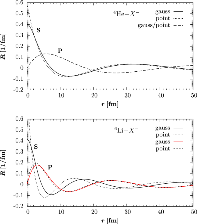
Following the outlined approach, we solve (2.7) for the relative motion of various – systems. As examples, we choose – and –. At the times of BBN the relative velocity of the /– system is Boltzmann distributed so that . Thus, a representative value is which corresponds to for with . We join the inner solution with the outer one at . This determines the phase shift . We have checked that is insensitive to the chosen value of , provided , and that when switching to a point-like nucleus. Using a Gaussian charge distribution, we find for the S-wave of the ()– system whereas for the P-wave the phase shift is already significantly reduced, .
In Fig. 2.3 the corresponding wave functions for – (top) and – (bottom) are shown. As can be seen, the wave functions for the case “gauss” receive a significant correction in comparison to the Coulomb case “point” which was already indicated by the size of the phase shifts . Of course, the curves labeled “point” coincide with the regular Coulomb functions [Eq. (2.12a)]. Whereas for the – system , a deviation from the regular Coulomb P-wave is visible in the – case.
When considering continuum wave functions for the numerical evaluation of (2.13) is problematic. This case, however, is the most important one in the computation of the photo-dissociation cross section of [Sec. 2.3.1]. Therefore, we need to consider the Coulomb wave functions in a different form [71],
| (2.17a) | ||||
| (2.17b) | ||||
where and are related to the Whittaker functions; . Defined in this way, (2.17) satisfy the asymptotic behavior (2.14). An expansion in powers of , i.e. in energy, for reads [71] (see also [72])
| (2.18a) | |||
| whereas cannot be represented by a convergent expansion in powers of energy. However, an asymptotic expansion has been obtained in [71], | |||
| (2.18b) | |||
Here, and are the respective Bessel functions of the first and the second kind of order [68] and the coefficients satisfy recurrence relations (); for details see [71]. With the expansion
| (2.19) |
one obtains from (2.18)
| (2.20a) | ||||
| (2.20b) | ||||
In the following section we employ those approximations in the computation of the photo-dissociation cross section.
2.3 Formation of bound states
The crucial quantity in the discussion of the catalysis of BBN reactions is the bound state fraction of the light elements . To this end we have to compute the cross sections for radiative recombination, , as well as for the dissociation, due to background photons .
The rate (per nucleus ) for – recombination is given by . Here, has to be averaged over the distribution of relative velocities between and which is Maxwellian for a sub- plasma,
| (2.21) |
Hence,
| (2.22) |
where has been used.
The rate of photo-dissociation of pairs depends on the number of photons whose energy exceed that of the ionization potential of the bound state,
| (2.23) |
and is given by .
The principle of detailed balance [34] relates the cross sections via where denotes the momentum of the relative motion of the –system and the factor of two is a statistical factor accounting for the two polarization degrees of freedom of the photon. From the definition of the rates and together with (2.22) and (2.23) it follows that444It is used that and that which holds well in the temperature regions of main interest.
| (2.24) |
As long as , i.e., as long as recombination and break-up reactions happen frequently, the concentrations of , , and have time to achieve equilibrium values such that the reaction densities for recombination and dissociation are equal, . This yields the Saha equation for the bound state fraction,555When used in this form one may need to impose that the number of bound states cannot be larger than the total number recombination partners available.
| (2.25) |
2.3.1 Photo-dissociation and recombination cross section
Since the early Universe is in a high-entropy state, bound states can only form efficiently once [73]. At the relevant times, i.e., when , only those photons in the high energy tail of the spectrum with are capable of destroying ; . In addition, the binding energy is significantly smaller than the associated light element mass so that a non-relativistic treatment of the photoelectric effect is perfectly justified.
For the computation of the photo-dissociation cross section we can employ Fermi’s golden rule. The probability per unit time for a nucleus bound to to undergo a transition into the continuum is given by
| (2.26) |
After the transition the nucleus has kinetic energy and momentum .666 Of course, strictly speaking, it is the energy and momentum of the relative motion. From the above explanations, however, it is clear that the recoil is negligible. The density of final states is and the matrix element for absorption of a photon with momentum and energy reads
| (2.27) |
where is the Fourier transform of the transition current and denotes the photon polarization vector; see, e.g., [48]. The cross section is found by dividing (2.26) by the incident photon flux density. Averaging over photon polarizations [in the gauge ], and integrating over , the differential cross section for photo-dissociation is given by
| (2.28) |
where is a unit vector in -direction and is the spatial part of .
We shall consider ionization from 1S as well as from 2S states. The initial state wave function is . The final state has to comprise a plane wave in direction together with an ingoing spherical wave [74]. In the partial wave expansion,
| (2.29) |
with unit vectors in -direction; are the Legendre polynomials [68]. Note the appearance of the additional phase shift coming from the finite charge radius correction.
| bound state | ||||||||
|---|---|---|---|---|---|---|---|---|
| 1870 | 4380 | 3980 | 0. | 6 | ||||
| 118 | 294 | (278) | 7260 | (9230) | 8. | 3 | ||
| 34 | (52) | 103 | (123) | 6640 | (25370) | 19. | 0 | |
Since the wavelength of the ionizing radiation ( on the threshold) is much larger than the dimensions, we can use the electric dipole approximation. The associated selection rule implies for the continuum so that
| (2.30) |
and thus (in the dipole approximation)
| (2.31) |
Performing all angular integrations in (2.28) yields for the total photo-dissociation cross section
| (2.32) |
For and we employ our numerically obtained solutions of the previous section which takes into account the finite charge radius of the nucleus. Note that on the ionization threshold is independent of . For a pure Coulomb field the momentum dependence cancels analytically when using the leading term in (2.20). By the same token, numerically, in (2.32) becomes insensitive to . Thus, we find a constant cross section for . In this limit, using detailed balance, the averaged recombination cross section reads
| (2.33) |
from which is readily obtained by using (2.24)
| (2.34) |
In Table 2.4 we present the results on the threshold photo-dissociation cross sections for transistions from 1S and 2S states for the elements , , and and for . The bracketed values are for a pure Coulomb potential whereas the other results are obtained by using a Gaussian charge distribution. The respective values do not differ very much. This is because the decrease of in the denominator of (2.32) when switching from the “point” to the “gauss” case is counterbalanced by an increase in the radial integral so that the net effect is small. However, the reduction of the total (1S+2S) recombination cross section from the hydrogen-like case is drastic. This is due to the additional factor of in (2.33). In the last column we show the temperature for which , i.e., the temperature when the formation of bound-states can proceed efficiently—provided that and that the bound state is not destructed by another process.
Finally, we remark that for other (heavier) nuclei than the ones presented in Table 2.4 the discussion of recombination can become more involved. If the light element possesses an excited state with a level splitting smaller than the binding energy, then recombination may also proceed into opening up the possibility of resonant recombination. This was pointed out in [75] where the formation of was considered.
2.4 Nuclear reactions with bound states and their catalysis
After the freeze-out of weak interactions with the cease of n and p interconversion processes, light element fusion in SBBN proceeds via inelastic two-body nuclear reactions777This does not include “production” processes like that of via electron capture by or of by beta decay of , both of which, however, only happen at a much later time.
with denoting the nuclei of the light elements and the arrow indicating the forward process, i.e., the exoergic direction with positive value. The reverse processes are typically suppressed by such as in (2.24) (which is an atomic process.) Only elements with atomic mass number are produced in relevant quantities.
In presence of bound states of the light elements with during BBN the following additional types of inelastic reactions emerge as particularly prominent,
A first observation is that, in presence of bound states, the energy gain of a nuclear reaction is altered. In the entrance channel, the total available internal energy is reduced due to the binding of with . Thus, for example, whereas additional energy becomes available in the exit channel of so that . Since values of nuclear reactions are mainly in the to multi- range, usually three-body break-up reactions rather than exit channels are realized. The shift in energetics can also allow for resonances which are not possible in SBBN. For example, type can be realized in resonant capture reactions whose intermediate excited state decays into the ground state by emission. If, instead, the nucleus is in an excited state , then also the continuum acts as a concurrent channel—provided that it is kinematically accessible. The latter is an example of a reaction of type which is of particular interest since it has no SBBN counterpart. Atomic reactions are called charge exchange reactions. They are also important to consider because they can significantly affect the relative concentrations of nuclei bound to . They will be discussed in Sec. 2.5.
Reactions of the form are only of secondary importance. Their efficiency depends on the average relative velocity between and which scales as . Thus, for weak scale relics, the suppression of the average velocity of -containing bound states relative to the velocity of light nuclei is from one to two orders of magnitude.
Another observation is that the screening of the charge of when in bound state with will lead to a modification of the SBBN cross sections with charged “projectiles” . It is customary to write the cross sections of charged-particle induced reactions in the form
| (2.37) |
and which defines the astrophysical -factor. The definition scales out the “geometrical” cross section as well as the Coulomb penetration factor . Note that during BBN () the thermal energy of the reactants is significantly smaller than the height of the Coulomb barrier ; is the de Broglie wavelength of the relative motion and denotes the earlier encountered Sommerfeld parameter [below (2.13)]. Using (2.37) the definition of the thermally averaged cross section (2.22) becomes
| (2.38) |
where is called the Gamow energy. In absence of resonances the -factor is only a slowly varying function of so that the integral is dominated by the exponential which peaks at and which marks the energy range of most effective nucleosynthesis (Gamow window).
One may then attempt to account for the bound state in the entrance channel by replacing by and correcting for the changed kinematics and energetics. Indeed, such a program has first been carried out in a BBN network calculation in [73]. When studying the effect on the charged particle induced reactions, the authors find no significant changes in the light element yields at the CMB inferred baryon asymmetry. Whereas the compactness of the bound states with the heavier of the light elements gives some justification to this procedure we will see in Sec. 2.5 that, e.g., the large size of the system plays a crucial role in obtaining a consistent picture of BBN.
2.4.1 Catalysis of 6Li production
The potential influence of bound states on the BBN paradigm was already discussed almost twenty years ago in [76, 77, 78]. However, only recently it has been realized [79] that the presence of at can lead to a tremendous enhancement of the output.
In SBBN the freeze-out of from nucleosynthesis is dominated by its production via radiative capture and its destruction via proton burning,
| (2.39a) | ||||||
| (2.39b) | ||||||
respectively. The cross section for the production reaction (2.39a) is very small with [80] at the lowest energies. For example, the -factor for which is the main source for at reads [81]. The small SBBN output of is attributed to the inefficiency of the production process (2.39a).888This is usually traced back to a weak quadrupole transition (E2) in (2.39a). Theoretical calculations seem to suggest, however, that at the BBN relevant temperatures the dipole transition (E1) is as important [82]. Nevertheless, the dipole moment of the – cluster is almost vanishing due to a similar charge-to-mass ratio which yields a very small cross section; cf. [79]. In this regard, also note that the destruction reaction (2.39b) has a large -factor, [80].
Let us briefly outline the evolution of the abundance in SBBN. Once the temperature of the primordial plasma drops below the deuterium bottleneck opens so that production can proceed via (2.39a). A sharp drop in below is accompanied by an associated decline in ; see left part of Fig. 2.4. Net production of via (2.39a) soon freezes out but proton burning (2.39b) continues until .
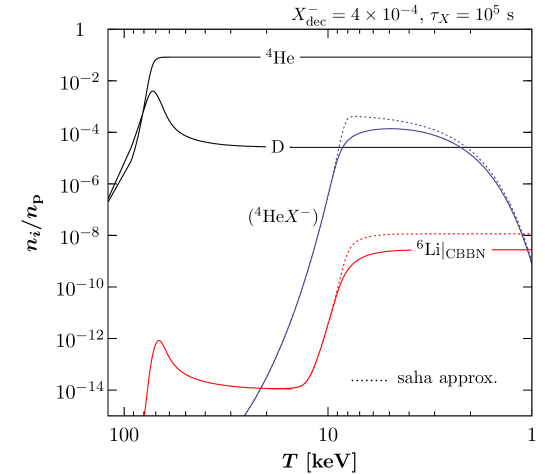
In the previous section we have seen that once the temperature drops below the photo-dissociation rate of freezes out. Thus, provided that is large enough, the concentration of can become substantial and fusion of is then possible via the alternative path [79]
| (2.40) |
and which is a reaction of type . Whereas the size of the radiative capture cross section (2.39a) is governed by the selection rules of the electromagnetic transition, (2.40) suggests a cross section which is determined by the short distance behavior of the – cluster. Indeed, the original work [79] estimates which points to a cross section for (2.40) which is in the ballpark of photonless SBBN reaction rates and implies the catalysis of production.
Meanwhile, a dedicated quantum three-body calculation of the system has become available [84] which confirms the catalytic picture. The authors find at the Gamow peak position . The thermally averaged cross section reads [84]
| (2.41) |
and is given in the customary units of ; denotes the temperature in units of and is the Avogadro constant [85].
Since only forms for , i.e., at a time when the and abundances are essentially frozen out, we can incorporate the effect of catalytic production in the following way. At some low temperature we couple the SBBN output into the network of Boltzmann equations
| (2.42a) | ||||
| (2.42b) | ||||
| (2.42c) | ||||
| (2.42d) | ||||
| (2.42e) | ||||
Light elements as well as bound state abundance are normalized to the baryon number, , , and —better overview shall compensate for the slight abuse of notation.
The central input parameter for the catalytic production of (and , see below) is the abundance of at the time of its recombination with . Above , we can track the resulting () abundance by using the Saha-equation (2.25) since photo-dissociation and recombination proceeds rapidly. Only at , () starts to build up efficiently so that we couple it into the full set of Boltzmann equations (2.42). We parameterize by its abundance prior to decay by introducing , where the superscript “dec” stands for decoupling, and by the lifetime , so that the (total) abundance at any moment during BBN is given by . The SBBN cross section for residual destruction (2.39b) can be found in [86]. We solve (2.42) using as initial conditions the SBBN output values of the computer code [83]: , , , and ; furthermore, and .
In Fig. 2.4 we show the evolution of the , , and number densities normalized to for the exemplary choice and . Rapid photo-dissociation delays bound-state formation of until . Once forms, catalyzed production proceeds efficiently via (2.40) which leads to the steep rise of at . As can be seen, the and reservoirs are essentially unaffected by this. In addition, the dashed lines show the and abundances when—instead of solving (2.42)—the Saha approximation (2.25) for the bound state fraction is used. This results in an overestimation of the output. The reason is that – recombination itself is efficient only for a short period after photo-dissociation freezes out. Thus, in order to obtain a reasonable estimate on , a numerical solution of the Boltzmann equations (2.42) is necessary.
2.4.2 Catalysis of 9Be production
Another dramatic catalytic enhancement is seen in the production of . The yield of in SBBN is tiny: Whereas the short lifetime of [see Sec. 2.2.1] renders the neutron capture reaction inefficient, production via fusion on Li isotopes yields no more than at [87]. The catalytic path to is shown by the following sequence [63]
| (2.43) |
which goes through the “double bottleneck” of and . Bound states () are formed by the radiative fusion
| (2.44a) | ||||
| and the catalysis of production is triggered by the photonless recoil reaction | ||||
| (2.44b) | ||||
The respective cross sections for (2.44a) and (2.44b) have been obtained in [63] and read
| (2.45a) | ||||
| (2.45b) | ||||
in units of . A comment is in order here. Recently, the catalytic path (2.43) has been questioned in [64]. On theoretical grounds it is argued that the charge radius of , , adopted in [63] is too small; see Sec. 2.2.1. Since the neutron capture reaction (2.44b) proceeds resonantly via the excited state , the larger charge radius as proposed in [64] decreases and shifts the resonance below threshold. A final answer on the efficiency of (2.44b) can only be obtained by a full quantum four-body calculation and is announced in [64] as work in progress.
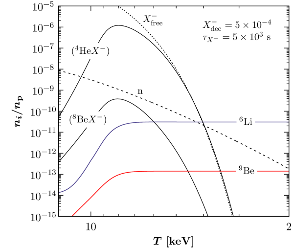
Given the unique sensitivity to physics beyond the Standard Model a primordial origin of offers, we choose to incorporate (2.43) into our reaction network. The following Boltzmann equations describe the production of ,
| (2.46a) | ||||
| (2.46b) | ||||
| (2.46c) | ||||
Again, as in (2.42), the abundances are normalized to and written in an obvious notation; . For , the SBBN neutron abundance can already be tracked well by including the processes , , and into the reaction network [88]. The respective cross sections , , and are taken from [86]. Note that at the time of catalyzed fusion the reservoir is essentially unaffected by those residual SBBN reactions so that we can neglect the back-reaction on (2.42e). The yields of and are taken from the output from an updated version of the Kawano code [89]. For the neutron lifetime we use [32].
In addition, we supplement the right hand sides of (2.42), (2.42), and (2.42) with
| (2.47a) | ||||
| (2.47b) | ||||
| (2.47c) | ||||
respectively. In our code we can neglect the formation of () that proceeds via molecular bound states () [63]. This process becomes important only for a combination of large and large , i.e., a parameter region which is already excluded by overproduction. Also note that at the time when () form, their photo-dissociation is not important because of the high binding energy ; see Table 2.3. It is important to note that we assume the SBBN value for the deuterium abundance. The early decays of may result in an injection of nucleons into the system. This typically drives the deuterium abundance upward, resulting in an enhanced number of neutrons at later times and therefore in an increased output of , with the general scaling . We choose to disregard this effect, noting its model-dependent character. We are allowed to do so since its inclusion can only make the -derived bound on the abundance stronger.
Figure 2.5 shows the evolution of catalyzed and production from the solution of the corresponding set of Boltzmann equations below keV. The curves in Fig. 2.5 are based on the values and . When the “bottle-neck” abundances of () and () form, the catalytic paths (2.40) and (2.43) to and open up, resulting in the asymptotic values and . The dashed line shows the neutron abundance and the dotted line the free abundance, which is dominated by its exponential decay. We remark in passing that residual recombinations of with lead to the crossing of the () and lines at late time.
2.5 Charge exchange reactions and late time catalysis
In this Section we discuss the role of bound states of with protons. The system may have a large impact on the BBN predictions because (i) the proton as a recombination partner is the most abundant element and (ii) it is a neutral system. As can be seen from Table 2.4, the recombination of bound states becomes efficient only after the temperature drops below 1 which corresponds to a cosmic time of . Thus, the question arises [76, 73, 90] whether a revival of fusion reactions, i.e., a late-time catalysis, can be triggered by the (potential) high reactivity of “neutron-like” bound states .
As we will see in Sec. 2.6 the presence of even a modest number density of during the recombination with helium can lead to a production of and at levels which are in stark conflict with their observationally inferred primordial values. In [90] it was claimed that large fractions of the previously synthesized at can indeed be reprocessed by via999At the time of publication of [90] the catalysis of production [63] had not yet been realized.
| (2.48) |
Thus, it was advocated that allowed “islands” reconcilable with observations may well exist in the abundance/lifetime parameter space for .
In the following we shall argue that this is not the case. One reason is that any arising abundance is immediately intercepted by the very efficient charge exchange reaction [76]
| (2.49) |
This reaction may have a very large rate as its cross section is determined by the actual size of the bound state that is of the order of ().
The charge exchange (2.49) can best be understood by employing a semi-classical picture. Calling the separation between and (or, more generally, the separation between and the incoming nucleus of charge ), the one-dimensional slice of the proton potential energy in the field of and is given by,
| (2.50) |
and is plotted in Fig. 2.6.
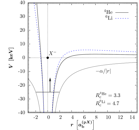
The limit of corresponds to an unperturbed binding of the proton to with a binding energy of . For and finite , the curve has a maximum at positive values of referred to as . As the nucleus comes closer, decreases. At some point, the binding energy of the proton becomes positive so that the tunneling of the proton to starts to become viable. For even smaller values of , one can find the distance at which the probability for the deconfinement of the proton approaches unity due to the fly-by of the nucleus. In order to estimate , we employ the variational calculation of the proton energy in the potential (2.50) by using the (unnormalized) trial wave function for the ground state,
| (2.51) |
where and are elliptic coordinates and and the minimization parameters. The coordinates are defined as and , where and are the proton–nucleus and proton– distances, respectively. We calculate the energy of the ground state as a function of the distance . This yields the critical separation , i.e., the distance at which , and which describes the situation when even a metastable bound state simply cannot exist.
The cross section for the charge exchange reaction may then be approximated by the geometric one with the impact parameter , . The deconfining distances together with the estimated cross sections for charge exchange are presented in Table LABEL:table-chex. The associated thermally averaged cross sections are given by and are listed in the Table LABEL:table-CBBN-rates found at the end of this Chapter.
| Z = 1 | Z = 2 | Z = 3 | Z = 4 | |
|---|---|---|---|---|
| 40 | 95 | 135 | 160 | |
| 51 | 280 | 580 | 850 |
As can be seen from Table LABEL:table-chex, a – distance of is sufficient to release the proton from the bound state. Consequently, the estimate points to a very large cross section of almost bn for the charge exchange reaction (2.49).
For the charge exchange on [Eq. (2.49)] an exact solution of the three-body Schrödinger equation has recently become available [64]. The authors confirm the efficiency of the charge exchange and find
| (2.52) |
This compares well with the estimate obtained from the semi-classical picture when evaluated at the fiducial temperature of .101010The different scaling of the averaged cross sections obtained in the semi-classical approach stems from the fact that their energy dependence has not been resolved; cf. [64]. Note that the charge exchange will mainly proceed into the level—preferentially with highest (largest number of states); cf. Table 2.2. Capture into highly excited orbits is indeed observed in charge exchange reactions of muons on hydrogen which gives justification to the employed semi-classical approach. Reference [90] finds for the charge exchange on a rate (per particle pair) of which is an underestimation by two to three orders of magnitude.
We incorporate the charge exchange reaction on in the network of Boltzmann equations by solving
| (2.53) |
for the abundance. The back-reaction on free protons is negligible so that we refrain here from writing an equation for . However, we need to supplement the right hand sides of (2.42), (2.42), and (2.42) by
| (2.54a) | ||||
| (2.54b) | ||||
| (2.54c) | ||||
respectively. Using the recent result (2.52) for the charge exchange cross section, we find that in the limit of infinite lifetimes, , the abundance of reaches its peak at around keV. Its maximum abundance at these temperatures can be well approximated as
| (2.55) |
where the assumption has been made [see Sec. 1.3] ensuring the linear scaling in (2.55).111111Using instead of (2.52) the cross section inferred from Table LABEL:table-chex yields the coefficient in Eq. (2.55); see [4]. That such a small fraction only has a marginal impact on can be seen by comparing the destruction rate for (2.48) [64]
| (2.56) |
to the Hubble rate at the relevant temperature of . Using we find
| (2.57) |
which tells us that the whole issue of mediated destruction of (and accordingly of ) is irrelevant so that the abundances of and fused at remain unaffected at .121212The same conclusion—prior to the publication of [64]—has already been reached in [4] by assigning the maximal possible rate for the destruction process (2.48) which is given by the unitarity bound.
We can further employ the results summarized in Table LABEL:table-chex. A successive chain of charge exchange reactions with can lead to molecular states that are finally destroyed in nuclear reactions with protons. In particular, has a chance for a nuclear interaction with protons or helium unsuppressed by a residual Coulomb barrier since it is a very compact object. We can solve for those molecular bound states by extending our network of Boltzmann equations for smaller than a few with
| (2.58a) | ||||
| (2.58b) | ||||
| (2.58c) | ||||
and supplement the right hand sides of Eq. (2.5) with
| (2.59a) | ||||
| (2.59b) | ||||
A similar chain exists for where the sequence of the charge exchange reactions can proceed until . It is important to note that the efficiency of this chain reaction depends very sensitively on the concentration of the bound states and on the mass of the particle. The latter enters through the average relative velocity of two heavy objects, e.g., and , which in turn scales as . Therefore, in the limit of an infinitely heavy , the chain will be cut off right at the first step, terminating at (). Also note that in (2.59b) we have made the assumption that is not destroyed by the decay of . Clearly some of the recoiling nuclei will be destroyed when released from the bound state. For the case of this has been investigated in [75] where it was found that no significant depletion of takes place. On those grounds and noting that only a small fraction of is locked in bound states with it is safe for us to disregard this effect.
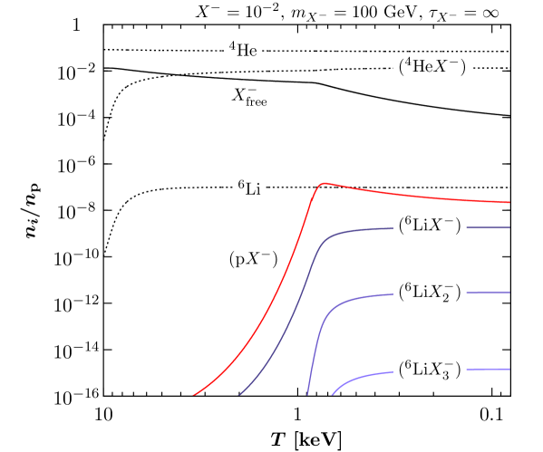
We run the full set of Boltzmann equations to determine the residual concentrations of and of the molecular bound states of with . The results are plotted in Fig. 2.7. As one can see, an initial concentration of per nucleon of results in a abundance that never exceeds the maximum (2.55), leading to a progressively diminishing number of molecular states.
We remark that for the computation of Fig. 2.7 we have not included formation via radiative recombination . This process is not important for the present discussion because it does not affect (2.55); is dominantly removed by charge exchange on . We have checked this by including the recombination process into our reaction network; cf. Table 2.4. Whereas would form around the same time as it is important to note that is also destroyed via hindering its formation; the corresponding cross section is given in [64] and in Table LABEL:table-CBBN-rates with the name . Even with we find that the final output is one order of magnitude below unbounded and (2.55) remains unchanged. By the same token, we find that the destruction process only has a minor impact on the total abundance (below 10%). For smaller values of the effect is accordingly weaker.
To conclude this section, neither lithium nor beryllium synthesized in CBBN processes at would be affected in any significant way by the subsequent generation of bound states. Thus—as we will show later—the part of the parameter space with a typical freeze-out abundance and a long lifetime will be confidently ruled out.
2.5.1 Relaxation after charge exchange
Above we have stated that the charge exchange on will mainly proceed into excited states of . Though we have already shown that bound states do not reach an abundance level where late-time catalysis plays a role it is nevertheless amusing to see whether receives further depletion by the energetic photons released from relaxation of from its excited states into the ground state. Upon transition into the ground state will be injected into the plasma in form of photons. This happens predominantly at and the photons loose their ability to break up once they are degraded below .
The rate for photon-photon scattering with —scaling with [91]—is rapidly becoming inefficient for at the relevant temperature so that we can neglect this photon-multiplying process. Thus, the photons loose their energy mainly by Compton scattering on background electrons. In the low-energy limit of Thomson scattering the mean lifetime of a photon before scattering is
| (2.60) |
where we have used ; see (1.45).
Since the energy loss of particles in Compton scattering is very small, we can write a differential equation for the systematic energy transfer to the electrons
| (2.61) |
Note that we have neglected a term which would account for the expansion of the Universe. We can do so since . The average energy loss per scattering is given by
| (2.62) |
At the rest frame of the electrons essentially coincides with the frame of the thermal bath. Then is given by the Klein-Nishina formula [92]
| (2.63) |
with
| (2.64) |
From (2.62) together with and it then follows that
| (2.65) |
Since the mean lifetime of the photon against Compton scattering is much shorter compared to the Hubble time we can integrate (2.62) from to by neglecting any associated drop in temperature of the plasma. This defines a typical escape time , i.e. a thermalization time-scale upon which the photon looses its ability to ionize . We find
| (2.66) |
This has to be compared with the mean lifetime of an energetic photon against ionization of ,
| (2.67) |
and which is of the order of the Hubble time; In the last step we have used as given in (2.55) with . The photo-dissociation cross section has been obtained in Sec. 2.3.1; see Table 2.4. This tells us that the thermalization of the injected photon happens very rapidly so that those photons released in the relaxation process after charge exchange are not capable of depleting any further.131313The numerical values of the various times-scales sensitively depend on the exact value of fiducial temperature chosen. However, the argument is not affected by that.
2.6 Constraints on the lifetime and abundance
In order to constrain the (, ) parameter space from the catalytic path (2.43) to [63], we need to set an upper limit on its primordial abundance from existing observations. It is generally accepted that the galactic evolution of the abundances of Be, along with Li and B, are dominated by cosmic-ray nucleosynthesis. While Be is burned rapidly in stellar centers, it is produced in cosmic rays by the spallation reactions of fast protons and particles hitting ambient CNO nuclei [93, 94]. As a consequence, the abundances of Be and O are linked, leading to a secondary scaling, Be [95]. On the other hand, inverse spallation reactions of CNO nuclei, both produced and accelerated in supernovae, will give a Be yield that is essentially independent of the metallicity of the interstellar medium. Such primary processes, leading to Be , are expected to play a major role during the early galactic epochs [96].
The produced Be is subsequently supplemented in the outer layers of stars. Thus, old stars which are far from the galactic center (and thereby less affected by the galactic chemical evolution) bear the potential to encode any pre-galactic origin of Be. Indeed, Be has been observed in a number of Population II halo stars at very low metallicities . Particularly noteworthy is the detection in the star G 64–12 at [97]. The star’s high Be value of might suggest a possible flattening in the Be trend during the early evolutionary phases of our galaxy [97]. Whether this really points to a primordial plateau or whether this indicates a Be dispersion at lowest metallicities [98] is not clear at present.
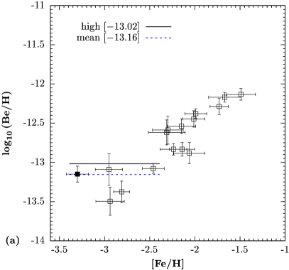
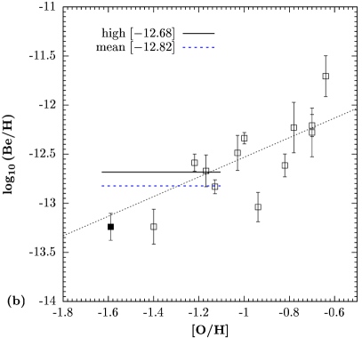
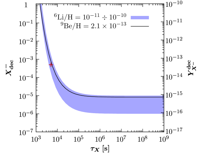
Figure 2.8a shows the original Be detection in the star G 64–12141414For consistency with the rest of the data points, the 1D LTE value has been plotted in Fig. 3a of the original reference [97]. (filled dot) along with a subset of data points taken from Fig. 3a of Ref. [97]. The data of Fig. 2.8b are taken from Fig. 6b of the recent work [99] which also uses as a metallicity tracer. The latter paper discusses the implications of a new temperature scale on the abundances of Li, Be, and B. In principle, different assumed physical parameters which characterize the stellar atmosphere may result in large systematic shifts of the inferred abundances. In this regard, it is important to note that Be is not overly sensitive to the assumed surface temperature of the halo dwarfs [99]. In the following we thus shall take a pragmatic approach: In both Fig. 2.8a and Fig. 2.8b, we obtain the least squares weighted mean (dashed lines) for a representative sample of stars at lowest metallicities. From the variance of the fit, we can extract a nominal upper limit (solid lines) on primordial . From Fig. 2.8b, we find
| (2.68) |
Conversely, Fig. 2.8a yields while fitting only the last two data points with in Fig. 2.8b would give . In our context, those values are less conservative so that we use (2.68) in the following. In Fig. 2.8b we have additionally fitted for a primordial component, , in combination with a primary scaling, . It seems, however, that a purely primary mechanism with fits the data best since comes out negligibly small.151515For a proper comparison between different assumed surface temperature scales and corresponding fits of primary versus secondary scaling, see Ref. [99]. Finally, we are aware that neither of the fitted mean values in Fig. 2.8 is very good in terms of . However, a firm conjecture of a Be plateau is not the purpose of this work, and indeed (2.68) does provide a sufficiently conservative limit to work with.
We can now confront the constraint (2.68) as well (1.6) with the CBBN yield of and obtained by solving the associated Boltzmann equations presented in Sec. 2.4 for a wide variety of (, ) combinations. In Fig. 2.9 we obtain exclusion boundaries from catalyzed and production in the (, ) parameter space. For convenience of the reader, the number density normalized to the entropy density, , is given on the -axis on the right-hand side. Above the solid line, is in excess with respect to (2.68) and thus excluded. The shown band reflects the uncertainties in the observational determination of . On the lower border, is fulfilled while holds on the upper border of the band. The cross indicates the exemplary parameter point considered in Fig. 2.5. At large lifetimes, the linear scaling of with can easily be seen from the boundaries of the band. Note that we find in the interval between and , whenever CBBN is efficient, which confirms the observation already made in Ref. [63].
| process | name | rate |
| Recombination and photo-dissociation: | ||
| Charge exchange: | ||
| [64] | ||
| 6Li destruction (from [64]): | ||
| 6Li and 9Be catalysis (from [84] and [63]): | ||
| † For consistency, the rates employed for match the ones from [4]. From our numerical evaluation [Table 2.4] the respective coefficients for and read and . | ||
Part II The gravitino-stau scenario
Chapter 3 Gravitinos as a probe for the earliest epochs
3.1 The gravitino-stau scenario
In the first part of this thesis we have discussed the implications of a generic electromagnetically charged massive particle species if it is present in the early Universe during/after the era of BBN (). If is a weak scale thermal relic, it freezes out from the primordial plasma at cosmic times so that the question of the origin of its longevity arises.
Long-lived charged particles can naturally emerge in supersymmetric (SUSY) extensions of the Standard Model. In scenarios in which the gravitino is the lightest supersymmetric particle (LSP), a long-lived may be realized if the lighter stau is the next-to-lightest SUSY particle (NLSP). Assuming conserved -parity in this work the stau NLSP will be typically long-lived because it can only decay into the LSP with Planck-scale suppressed couplings. Conserved -parity also implies that the gravitino is stable which makes it a promising dark matter candidate.111The gravitino can also be dark matter if -parity is broken as long as it is ensured that the -lifetime is of the order of the age of the Universe; see, e.g., [100, 101, 102, 103] and references therein.
In this part of the thesis we consider gravitino dark matter scenarios in which the is the NLSP. In the present chapter we briefly introduce the gravitino and discuss immanent cosmological implications which are independent of the nature of the NLSP. In the next chapter we then work out the phenomenology of the gravitino-stau scenario.
3.2 Supergravity and basic properties of the gravitino
In ordinary gauge theories the generators of the of the Poincaré algebra commute with the generators of the internal (local) symmetry such as, e.g., color in the Standard Model. Indeed, it was shown [104] that any such extension of the Poincaré algebra in a four-dimensional quantum field theory (with non-zero scattering amplitudes) is necessarily trivial in the sense that both algebras decouple.
Supersymmetry, however, is an extension of the space-time symmetry which relates fermionic and bosonic degrees of freedom. The associated particles form a supermultiplet. The spinorial supersymmetry generator obeys anti-commutation relations and the (simplest) supersymmetry algebra reads222We follow the conventions used in [105]; and denote the commutator and anti-commutator, respectively.
| (3.1a) | ||||
| (3.1b) | ||||
| (3.1c) | ||||
Note that (3.1a) relates with the Poincaré algebra; generates translations. Therefore, local supersymmetry implies local Poincaré symmetry, i.e., invariance under general coordinate transformations. This is exactly what we expect from a theory of gravity so that local supersymmetry is also referred to as supergravity. The gauge field of supergravity is the gravitino. It is a spin-3/2 Majorana particle and can be written as a vector-spinor .
Particles within the same supermultiplet are degenerate in mass because . Since we do not yet have experimental evidence for supersymmetry, we know that it has to be a broken symmetry if realized in nature. Local supersymmetry offers the appealing possibility to be broken spontaneously with a super-Higgs mechanism operating. The Goldstone fermion of supersymmetry breaking is absorbed by which thereby acquires its longitudinal, helicity degrees of freedom. After supersymmetry breaking the gravitino has mass . Depending on the underlying breaking mechanism, can range from the eV scale up to scales beyond the TeV region [106].
The phenomenology of the massive gravitino is then governed by the following Lagrangian
| (3.2) |
The first two terms describe a free massive spin-3/2 field [107] from which it can be shown that the free gravitino field satisfies the Dirac equation for each component and is subject to the constraints and . The interaction Lagrangian reads333For an explicit “derivation” of from the general supergravity Lagrangian see [108].
| (3.3) |
Focusing on a minimal particle content in the observable sector, the fields , , and denote the gauge eigenstates of the scalars, chiral fermions, and gauginos of the MSSM; is the field strength tensor of the gauge group with index of the associated adjoint representation and denotes the gauge-covariant derivative. All matter fields are written in terms of left-handed four-spinors since they stem from left-chiral supermultiplets in the general supergravity Lagrangian [109]. For example, a right handed tau lepton is written in terms of its charge conjugate which is a left-handed spinor. Analogously the superpartner of is written in (3.2) as . Details aside, most important is the fact that the interactions of the gravitino to the MSSM fields are fixed by the (super)symmetry and are suppressed by inverse powers of which makes an extremely weekly interacting particle.444Couplings of a very light gravitino can be enhanced due to its longitudinal (goldstino) modes [110]—a remnant of the super-Higgs mechanism.
Being the gauge field of supergravity, the gravitino sits at the heart of any locally supersymmetric theory. Despite its extremely weak interaction gravitinos can be efficiently produced in the early Universe. In the next section we discuss the case of thermal gravitino production—a guaranteed source of potential relic gravitinos.
3.3 Thermal gravitino production and reheating
The observed flatness, isotropy, and homogeneity of the Universe suggest that its earliest moments were governed by inflation [111, 112]. The inflationary expansion is followed by a phase in which the Universe is reheated. The reheating process repopulates the Universe and provides the initial conditions for the subsequent radiation-dominated epoch. The reheating temperature can be viewed as the initial temperature of this early radiation-dominated epoch of our Universe.
The value of is an important prediction of inflation models. While we do not have evidence for temperatures of the Universe higher than (i.e., the temperature required by primordial nucleosynthesis), inflation models can point to well above [112, 113]. While any initial population of gravitinos must be diluted away by the exponential expansion during inflation [114], gravitinos are regenerated in scattering processes of particles that are in thermal equilibrium with the hot primordial plasma. The efficiency of this thermal production of gravitinos during the radiation-dominated epoch is sensitive to [115, 116, 117, 118, 108, 119, 120].
Gravitinos with have decoupling temperatures of , as will be shown below. We consider thermal gravitino production in the radiation-dominated epoch starting at assuming that inflation has diluted away any initial gravitino population.555 In this work, we neglect gravitino production in inflaton-decays, cf., e.g., [121, 122, 123] and references therein. Though this non-thermal source can give a sizable contribution it is model-dependent and typically small when considering high reheating temperatures with the associated gravitino yield scaling as [123]. For , gravitinos are not in thermal equilibrium with the post-inflationary plasma. Accordingly, the evolution of the gravitino number density with cosmic time is described by the following Boltzmann equation [108, 119]
| (3.4) | |||
| (3.5) |
The collision term involves the gaugino mass parameters , the gauge couplings , and the constants and associated with the gauge groups U(1)Y, SU(2)L, and SU(3)c as given in Table 3.1.
| gauge group | ||||||
|---|---|---|---|---|---|---|
| U(1)Y | 1 | 11 | 1.266 | 0.653 | 11 | |
| SU(2)L | 2 | 27 | 1.312 | 1.604 | 1 | |
| SU(3)c | 3 | 72 | 1.271 | 4.276 | -3 |
In expression (3.5) the temperature provides the scale for the evaluation of and . The given collision term is valid for temperatures sufficiently below the gravitino decoupling temperature, where gravitino disappearance processes can be neglected. A primordial plasma with the particle content of the MSSM in the high-temperature limit is used in the derivation of (3.5).
The collision term (3.5) results from a consistent gauge-invariant finite-temperature calculation [108, 119] following the approach used in Ref. [118]. Thus, in contrast to the previous estimates in [115, 116], the expression for is independent of arbitrary cutoffs. Note that the field-theoretical methods of [124, 125] applied in its derivation require weak couplings, , and thus high temperatures .666For an alternative approach see [120]. Thus, in the following we focus on cosmological scenarios with which is also the most attractive temperature range, e.g., for baryogenesis scenarios based on leptogenesis.
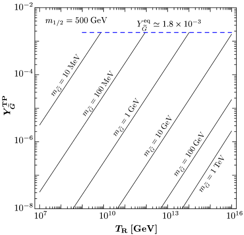
Assuming conservation of entropy per comoving volume, the Boltzmann equation (3.4) can be solved to good approximation analytically [118, 126]. At a temperature , the resulting gravitino yield from thermal production reads
| (3.6) | |||||
where the constants are given in Table 3.1. These constants are obtained with an effective number of relativistic degrees of freedom of which follows from the fact that the entire MSSM particle content is in thermal equilibrium and relativistic. We evaluate and using the one-loop evolution described by the renormalization group equation in the MSSM [106]:
| (3.7) | ||||
| (3.8) |
with the respective gauge coupling at the Z-boson mass, , and the coefficients listed in Table 3.1. For convenience we choose to parameterize the gaugino masses in terms of their values at the scale of gauge coupling unification . We remark in passing that when considering only the SUSY-QCD contribution in (3.6) it is sometimes also convenient to express the gravitino abundance in terms of the physical gluino mass [118]. As has been shown in [127] it is then important to employ a two-loop running of the gluino mass since using (3.8) for the renormalization group evolution from the electroweak scale to would underestimate the gravitino abundance by a factor of two. In this work, however, we use the running gluino mass at as input where the effect is smaller (and working in the other direction.)
For a standard cosmological history without release of entropy, the gravitino yield from thermal production at the present temperature is given by . The resulting density parameter of thermally produced gravitinos reads
| (3.9) |
with [32].
In Fig. 3.1 the result (3.6) for the thermally produced gravitino yield is shown as a function of for various values of (solid lines). The curves are obtained with for the case of universal gaugino masses at : . The dashed (blue) horizontal line indicates the equilibrium yield
| (3.10) |
which is given by the equilibrium number density of a relativistic spin-1/2 Majorana fermion, . For , since the spin-1/2 components of the gravitino are in thermal equilibrium. In the region where the yield (3.6) approaches the equilibrium value (3.10), gravitino disappearance processes should be taken into account. This would then lead to a smooth approach of the non-equilibrium yield to the equilibrium abundance. Without the back-reactions taken into account, the kink position indicates a lower bound for . Towards smaller , decreases due to the increasing strength of the gravitino couplings. For example, for (), we find ().
3.3.1 Reheating phase
In the analytical expression (3.6) we refer to as the initial temperature of the radiation-dominated epoch. So far we have not considered the phase in which the coherent oscillations of a field dominates the energy budget of the Universe and where one usually relates to the decay width of . In the simplest models of inflation the decaying field which reheats the Universe also drives the exponential expansion of the Universe. In the following we shall simply refer to as the inflaton field.
We can account for the (perturbative) reheating phase, by considering (3.4) together with the Boltzmann equations for the energy densities of radiation and the inflaton field,
| (3.11a) | ||||
| (3.11b) | ||||
respectively. To relate with we first note that the second term on the left hand side of (3.11b) indicates that (when averaged over several oscillations) scales like matter, ; denotes the scale factor. Thus, in terms of the initial inflaton energy density , the Hubble rate is given by
| (3.12) |
as long as dominates. Assuming an instantaneous conversion of into radiation when with usually chosen to be a number between and then allows one to define a reheating temperature in terms of the decay width of the inflaton field,
| (3.13) |
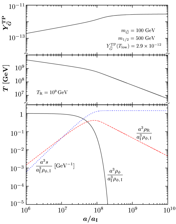
In Fig. 3.2 we show the results of a numerical integration of (3.4) and (3.11) plotted against the scale factor with chosen such as to yield for .777For the actual integration we rewrite the Boltzmann equations (3.4) and (3.11) in terms of dimensionless quantities following [128]. In the lower figure we plot comoving quantities normalized to . At the inflaton energy density decays exponentially and the Universe enters the radiation dominated epoch which can be seen by the turn-over of the dashed curve depicting the radiation density: there, starts to scale as . This is also indicated by the evolution of the temperature plotted in the middle part of the figure. In the radiation dominated Universe scales with . Also note that is not the maximum temperature of the Universe. When the inflaton field decays entropy is produced (dotted line in lower part) and the temperature scales as . The production of entropy is also the reason why in the top part of the figure—despite the large initial temperature—reaches its maximum value only in the radiation dominated regime when is finally constant. Here, at with and has been chosen which gives a final gravitino abundance of .
With our result for the collision term (3.5), we find that the gravitino yield obtained numerically is in good agreement with the analytical expression (3.6) for . For an alternative definition with different the associated numerically obtained gravitino yield is described by the analytical expression obtained after substituting with in (3.6).
A fitting formula on the gravitino yield which also includes the effect of reheating and which was based on [118] has been derived earlier in [47]. However, the production of the helicity-1/2 component of the gravitino was neglected so that the actual yield for was underestimated by about an order of magnitude. Accordingly, the bounds given in [47, 41, 129] are underestimated in the region . Meanwhile—after publication of [1] on which this section is based on—an updated treatment [130] has become available in which the authors now include the helicity-1/2 components as well as the electroweak contributions [108, 119] of the thermal gravitino production. For a most recent discussion on gravitino production during perturbative reheating see also [131].
3.4 Constraints on
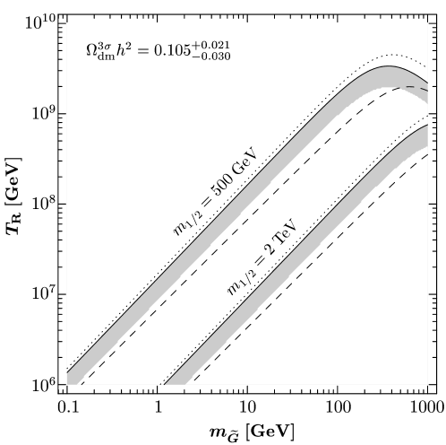
Since for the gravitino LSP the resulting density should not exceed the dark matter density , is bounded from above [116]. Such a bound has to be compared with predictions of the reheating temperature from inflation models. Moreover, is important for our understanding of the cosmic baryon asymmetry. For example, successful standard thermal leptogenesis [133] can typically require [134, 135].
We update the limits using the full gauge-invariant result for the relic density of thermally produced gravitinos, , to leading order in the Standard Model gauge couplings [108, 119].888The computation of the electroweak contributions to thermal gravitino production was subject of the diploma thesis [108] of the author in which similar limits on were already presented—however, without insight on the exact sensitivity of on the reheating process; in this section . In particular, this allows us to illustrate the dependence of the bounds on the gaugino-mass relation at the scale of grand unification .
The reheating temperature is limited from above in the case of a stable gravitino LSP since cannot exceed the dark matter density . In the following we use [7, 32] the WMAP 3-year result
| (3.14) |
In Fig. 3.3 we show the resulting upper limits on using as a function of . On the gray band, the thermally produced gravitino density (3.9) is within the nominal range (3.14). The upper (lower) gray band is obtained for at with (). From the requirement the dashed lines show the constraints for the exemplary non-universal scenario [136] at . Using the same requirement the dotted lines show the SU(3)c contribution [118, 132] for at . As can be seen by comparing the dashed and dotted lines, the electroweak contributions can be particularly important for the case of non-universal gaugino masses at . On the other hand, for gaugino masses which unify at , the dotted lines provide already a very good estimate. In this regard, note that Fig. 3.3 is updated from the one presented in [1] since the SU(3)c contribution to , originally obtained in [118], has meanwhile been corrected by the authors [132]. For completeness, we also remark that, after publication of [1], the upper limits on shown in Figs. 5 and 6 of Ref. [137] have also been corrected. Previously, these figures underestimated the maximal value of by a factor of four in the region in which governs the limits.
The limits shown in Fig. 3.3 are conservative bounds that do only depend on and the values at . Taking into account contributions to from NLSP decays will make those limits stronger. In the next chapter, we will account for this non-thermal gravitino source in a systematic way.
Chapter 4 The stau as the NLSP
In this chapter we now specialize on gravitino dark matter scenarios in which the lighter stau is the NLSP. Indeed, the appearance of as the lightest Standard Model superpartner is a commonplace occurrence even in models with restrictive assumptions on the SUSY breaking sector such as the CMSSM. The associated parameter region is usually not considered because of severe upper limits on the abundance of massive stable charged particles (see Sec. 1.3). However, in gravitino LSP scenarios is unstable and thereby a viable option.
In this chapter, we first review the result on a frequently used range of thermal freeze-out abundances of . Employing such an estimate allows us to constrain the gravitino-stau scenario from BBN limits on the electromagnetic and hadronic energy release in the decay of in a rather model-independent fashion. Moreover, we employ the results of Chapter 2 on the catalyzed light element production of and . We shall see that the associated constraints pose the henceforth strongest limits on this scenario. Specializing to the case of the CMSSM allows us to explore concrete realizations of the gravitino-LSP stau-NLSP setting. In particular, we shall find that the reheating temperature is heavily constrained by the novel CBBN bounds. We also explore the possibility of a non-standard cosmological history to see whether one can alleviate or even circumvent the strong restrictions on the parameter space.
4.1 Generic constraints on the gravitino-stau scenario
In order to set constraints on the outlined scenario we require knowledge on the stau abundance in the early Universe. In Sec. 1.3 we have found that for a standard cosmological history the decoupling temperature of a weak scale charged particle satisfies . Thus, with a post-inflationary reheating temperature above the decoupling temperature, the NLSP freezes out of the primordial plasma as a cold thermal relic so that its yield after decoupling is governed by its mass and its annihilation rate. Thereby, becomes sensitive to the mass spectrum and the couplings of the SUSY model and representative values
| (4.1) |
have been used to confront the gravitino-stau scenario with cosmological constraints [31, 138, 139, 2, 140]; denotes the mass of the lighter stau. Equation (4.1) compares well with our upper bound (1.15) derived from a purely dimensional analysis. The yield (4.1) with a coefficient is in good agreement with the curve in Fig. 1 of Ref. [31] that has been derived for the case of a purely ‘right-handed’ NLSP with a mass that is significantly below the masses of the lighter selectron and the lighter smuon, , and with a bino-like lightest neutralino, , that has a mass of . In the case of an approximate slepton mass degeneracy, , the upper value in (4.1) becomes saturated due to slepton coannihilation processes [31]. We shall see in Sec. 4.2.3 that approaching the – coannihilation region, , even larger enhancement factors occur. On the other hand, a sizable left–right mixing of the stau NLSP is associated with an increase of its MSSM couplings and thus with a reduction of . This will be discussed in Part III where a systematic investigation of the stau abundance and its sensitivity on the SUSY parameters will be given. In this section, we shall focus on the more generic values described by (4.1).
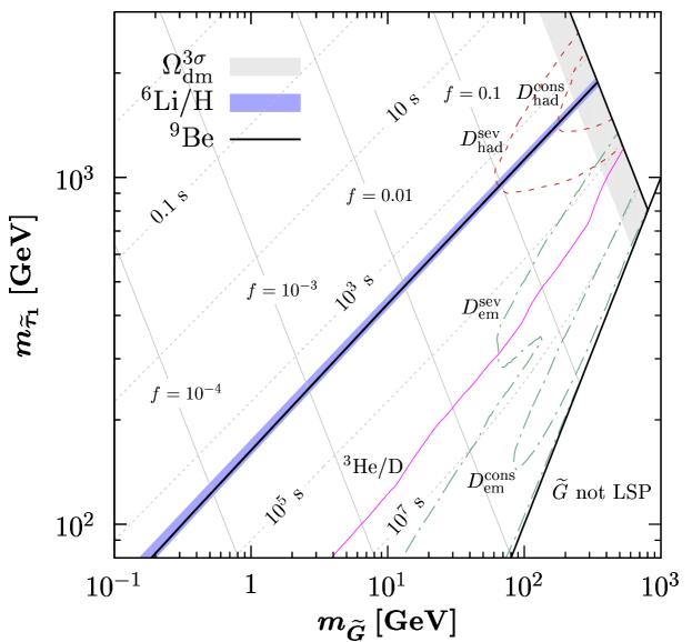
In Fig. 4.1 we collect the cosmological constraints on the gravitino-stau scenario by plotting versus . Let us go through the respective limits one by one:
- Non-thermal gravitino production
-
Each NLSP eventually decays into one LSP leading to a non-thermally produced (NTP) gravitino density [31, 141]:
(4.2) This contributes to the relic gravitino density which should not exceed the observationally inferred dark matter density . In Fig. 4.1 we choose as representative value
(4.3) In the light shaded region in the upper right corner agrees with of Eq. (3.14). The shading is limited from above by a solid line which borders the above disfavored region in which . Any additional contribution to , such as a thermally produced gravitino density (Sec. 3.3), makes this constraint more restrictive. This is indicated by the thin gray lines labeled with , , , and , on which (4.2) obtained with (4.3) satisfies , respectively. The timing of the NLSP decay into the gravitino LSP is governed by the two-body decay mode and reads
(4.4) in the limit . Contour-lines thereof are shown in Fig. 4.1 by the dotted gray lines. Starting from the upper left edge, they correspond to lifetimes of and then—as labeled—to , , , , and .
- CBBN constraints
-
We can now incorporate the results of Chapter 2 on the catalyzed fusion of and triggered by the bound state formation of . We use the CBBN constraints obtained in Fig. 2.9 with , i.e., we assume that there exists no asymmetry between positively and negatively charged staus [cf. Sec. 5.6]. For we use the estimate (4.3). The shaded region in Fig. 2.9 has corresponded to a output of and which is now likewise associated with the dark (blue) shaded band in Fig. 4.1. On the upper border of the band a lithium abundance of is attained whereas on the lower border holds. The region below the band is confidently ruled out by overproduction of .111Using the initial estimate [79] on the CBBN output, the associated constraint has first been shown in the -plane in [142]. Likewise, in this representation, the constraints from hadronic -decays have first been obtained in [141]. However, both works [141, 142] are based on outdated light element yields so that we use our treatment of Chapter 2 for and the update in [139] for the hadronic -decays. Moreover, we also show the CBBN constraint from primordial production which excludes a very similar region.
- Hadronic energy release
-
In Sec. 1.4 we have provided an overview over the physics of late decaying particles during/after BBN. In our concrete scenario we can now implement the stringent constraint on hadronic energy release from the observationally inferred primordial deuterium abundance.222Additional constraints on hadronic energy release are imposed by the primordial abundances of 4He, 3He/D, 7Li, and 6Li/7Li [143, 45, 40, 41, 144, 145]. However, in the region allowed by the 9Be and 6Li constraints from bound-state effects, i.e., , the considered D constraint on hadronic energy release is the dominant one as can be seen, e.g., in Figs. 38–41 of [41] and in Figs. 6–8 of [144]. The limits are based on the severe and conservative upper bounds on the product [here, ] obtained in Fig. 39 of [41] for (see references cited in [41]):
(4.5a) (4.5b) Recall from our discussion in Sec. 1.2 that (4.5b) is a rather high value on . Without trying to give extra credence to (4.5b), following [41], we simply take it as a limiting value for D/H. The average injected hadronic energy has been obtained in [139] from computation of the 4-body decay of the stau NLSP into the gravitino, the tau, and a quark-antiquark pair for a purely right-handed NLSP. The effect of hadronic energy injection on primordial D disfavors the regions inside the dashed lines shown in Fig. 4.1; see also Fig 16 in [139].
- Electromagnetic energy release
-
The constraints resulting from the dissociation of light elements due to interaction with the electromagnetic cascades formed in stau decays are obtained for a “visible” electromagnetic energy of of the tau energy
(4.6) released in . The and constraints result from the limits given in Fig. 42 of Ref. [41] and the constraint from the limit given in Fig. 6 of Ref. [39] . It is the region to the right or inside of the dot-dashed (green) curves and the region to the right of the and thin solid (pink) line that are disfavored by the primordial abundances of D and 3He/D, respectively.
As can be seen in Fig. 4.1, the constraints from the catalytic production of and are (essentially) the most restrictive ones. Their coinciding position is due the fact that the catalytic production of and both depend on (same timing) and that their output scales linearly in . Indeed, the associated constraints run parallel and in vicinity of the contour which corresponds to the time at which formation starts to become efficient. For the adopted stau abundance (4.3) this implies that lifetimes in the vicinity of are disfavored.
The electromagnetic and 3He/D constraints are always less restrictive than the CBBN constraints from 9Be and 6Li. Only the hadronic constraint competes with the CBBN constraints for , i.e., in the lifetime region in which is largest. Though for lifetimes shorter than about 100 s neutron-to-proton interconversion processes affect , the associated constraint is about two orders of magnitude weaker (as can be seen in left panel of Fig. 1.1). We also remark that the elevated content of D due to hadronic and electromagnetic energy injection leads to an enhancement of CBBN-produced and . For example, if non-thermal processes boost the deuterium abundance to the level of (4.5b), it would lead to an enhancement of the output by a factor of , while the corresponding enhancement factor in the case of is about 4. We have not included this effect since it can make our obtained limits only stronger.
Here we would like to emphasize that the 9Be and 6Li constraints are the ones that are the least sensitive to the precise value of in the region . This results from the fact that the limits are very steep in that region, as can be seen in Fig. 2.9. Indeed, a yield that is twice as large as (4.1) will affect the position of the 9Be and 6Li constraints only very mildly. In contrast, such an enhanced yield—as encountered, e.g., in the case of slepton coannihilations—leads to significant changes of the dark matter constraint and the BBN constraints associated with hadronic/electromagnetic energy injection, as can be seen explicitly in Fig. 16 of Ref. [139].
It should also be noted that an elevated slepton yield can lead to an additional non-thermal output of for . As discussed before, this is because energetic spallation debris of destroyed nuclei from slepton decays can hit ambient and thereby fuse [40, 41, 144]. This mechanism depends sensitively on the hadronic branching ratio of the 4-body slepton decay into the gravitino, the associated lepton, and a quark-antiquark pair for which typically for (see Fig. 5 of Ref. [139]). Indeed, as discussed in Ref. [146], for those branching ratios, the effect of CBBN on is the dominant one in the region which is not already excluded by the D constraint. Thus, for , our obtained limits on overproduction are only marginally affected by the hadronic energy release of -decays. However, for larger slepton masses, i.e., for scenarios of large in conjunction with , the hadronic production of becomes efficient so that only a simultaneous treatment of both effects can decide on the accurate BBN output.333Using the catalysis of BBN reactions in order to seek for a simultaneous solution of both, the and problem [cf. Sec. 1.1] has, e.g., been made in [145, 90, 75]; for a most recent discussion which also includes the lithium output due to decays see [42]. Note that this can make our presented limits on only stronger. Thus, we are on the conservative side when neglecting such additional contributions. We note in passing that with a highly fine-tuned - degeneracy leading to , any bound on energy release can be evaded. However, the CBBN bounds remain.
Let us also comment on the reliability of the novel CBBN constraints from and overproduction and address the implications of the associated restrictions on the parameter space:
- Reliability of CBBN constraints
-
As already emphasized in Sec. 1.1, observations of are extremely difficult. Whereas in the cold interstellar medium the lines of and are well resolved, measurements of the isotopic ratio in the outer layer of stars is complicated because the absorption lines of are not resolved spectroscopically with respect to the lines of due to thermal blending [18]. Indeed, the claim of a “-plateau” is being challenged in the recent papers [147, 148]. The presence of is inferred from an enhancement of the “red wing” of the absorption line. It is argued that such a line asymmetry could also be mimicked by Doppler-shifts due to atmospheric convective motions. Accordingly, some of the observations may eventually turn out to provide only upper limits. Moreover, is more fragile than and would burn more efficiently at lower temperatures. Therefore, if there is a (yet unconfirmed) stellar mechanism (see, e.g., [149]) that resolves the lithium problem, i.e., that depletes by a factor of two or three, would have been depleted by a larger factor.
Given those issues, we have adopted here a generous range on the observationally inferred upper limit on primordial with being a very high value. In this regard it is also important to note that the catalytic effect on is very strong so that—for the purpose of setting constraints—we are not overly sensitive to the precise value of the upper bound. This can be seen by the fact that the dark shaded (blue) band in Fig. 4.1 is rather thin while spanning one order of magnitude in fused . In this respect, Sec. 2.5 becomes important in which we show that the destruction of large fractions of the previously synthesized by is not feasible. This rules out the possibility that allowed islands in the parameter region with large /large —which was advocated to remain viable in Ref. [90]—exist.
Unlike , is firmly detected in a significant number of stars at low metallicity, and its observational status is not in doubt. (For the latest data on the abundance in metal-poor stars, see, e.g., [97, 150, 151, 98].) Also note that stellar depletion would affect less than either or since both and are more fragile than . Moreover, the nuclear physics rates that enter in the calculation of catalysis are dominated by resonances. Given the wealth of experimental information on the resonances [152, 153], this may eventually allow for very reliable calculations of the catalytic rates. Though it has recently been argued that the resonance in the final step (2.44b) in the fusion of is shifted below threshold [cf. Sec. 2.4.2] it is a neutron induced reaction so that such a shift will affect the efficiency of the reaction but may not be fatal. Moreover, also note that we have adopted a very conservative upper limit on primordial in (2.68) which can already be seen by mere optical inspection of Fig. 2.8b. Taking as a grain of salt that the final efficiency of the reaction is not fully established but noting the powerful physics potential a primordial origin of offers we have chosen to incorporate this constraint. Moreover, given the fact that both, and , show the same sensitivity on the gravitino-stau parameter space any conclusions drawn from are only corroborated and not altered by . We eagerly await further investigation of the critical catalyzed nuclear rates which shall give a final answer on the CBBN output of .
- Implications of CBBN constraints
-
From Fig. 4.1 it is immediately clear that the new CBBN constraints imply a lower limit on given . Clearly, a minimum value of the lightest Standard Model superpartner directly affects the testability of such SUSY scenarios at future colliders.
For the gravitino dark matter scenario in which is exclusively provided by , i.e., which are situated in the light gray shaded band, formerly (marginal) allowed islands with and are now confidently ruled out. Moreover, considering other values than the gravitino mass is constrained to values well below 10% of the slepton NLSP mass for . Thereby the kinematical determination of proposed in [154] remains cosmologically disfavored at the next generation of particle accelerators.
Of course, the CBBN constraints only emerge if is large enough to allow for bound state formation. Thereby, scenarios with a gravitino mass of and —the latter of which is supported by the non-observation of long-lived charged sleptons at the Large Electron Positron Collider (LEP) [32]—are unconstrained from CBBN. Accordingly, for gauge-mediated SUSY breaking which typically predicts small values of , the CBBN constraint can be irrelevant. However, in gravity-mediated SUSY breaking the gravitino mass sets the scale for the soft breaking parameters so that are the most natural values. Then, the CBBN constraints impose a lower limit of .
To extract further implications from the gravitino-stau scenario we resort in the next section to concrete supersymmetric realizations by full specification of the SUSY parameters. Thereby we obtain further insight on the superparticle mass spectrum. Moreover, this allows us obtain a stringent upper bound on the reheating temperature of the Universe.
4.2 The gravitino-stau scenario in the CMSSM
We now consider gravitino dark matter scenarios in the framework of the CMSSM where one assumes universal soft SUSY breaking parameters at . The CMSSM yields phenomenologically acceptable spectra with only four parameters and a sign: the gaugino mass parameter , the scalar mass parameter , the trilinear coupling , the mixing angle in the Higgs sector, and the sign of the higgsino mass parameter .
In the CMSSM with the gravitino LSP, the next-to-lightest SUSY particle is either the lightest neutralino or the lighter stau .444A stop NLSP is not feasible in the CMSSM [155]. The BBN constraints on electromagnetic and hadronic energy injection disfavor the NLSP for [141, 156, 137]. For the slepton NLSP case, the BBN constraints associated with hadronic/electromagnetic energy injection have also been estimated and found to be much weaker but still significant in much of the parameter space [141, 156, 137, 139]. In the following, however, we shall see that the novel CBBN constraints drastically change this picture.555Seeking a solution to the lithium problems, bound state effects within the framework of the CMSSM have first been considered in [145]. We set a different focus: We constrain the CMSSM parameter space from which we mainly derive an upper bound on .
Let us give an overview of what is presented in the remainder of this chapter. In Sec. 4.2.1 we consider the CBBN restrictions on the lifetime. Employing the results on from a renormalization group analysis this allows us to relate the stau mass with the high-scale parameter . The obtained lower limit on the latter parameter can be translated into an upper bound on the reheating temperature. This will be done in Sec. 4.2.2. Both limits will be based on the estimate (4.3) of the stau decoupling yield. We contrast the obtained semi-analytical limits on and with exemplary CMSSM parameter scans in Sec. 4.2.3. For those examples we will also explicitly consider in Sec. 4.2.4 the possibility of a non-standard cosmological history. In this context, we also check on the viability of thermal leptogenesis in Sec. 4.2.5.
4.2.1 Lower limit on
In the previous section we have realized that the new bounds emerging from the thermal catalysis of nuclear reactions yield the most dominant restrictions on the gravitino-stau parameter space. We have also noted that the discussion of those bounds is facilitated by the fact that both, the constraint on as well as the one on production, essentially disfavor the same region in the parameter space. In the following we focus on and adopt as an upper limit on its primordial abundance
| (4.7) |
We thereby resort in this work to a more conservative point of view than in our main discussions of the published works [1, 2, 3] which were based on [39]. In this way, we give account to the concerns cast in the previous section (without, however, going to the very extreme using .)
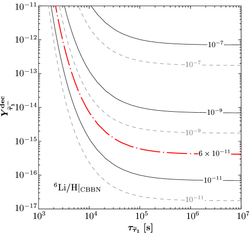
The limit (4.7) is shown by the dash-dotted (red) line in Fig. 4.2 as a function of the yield of negatively charged staus and . As in Fig. 2.9 the curve is obtained by numerical integration of the Boltzmann equations presented in Chapter 2. In addition, the solid lines show contours of constant output for other values than (4.7) as labeled. Moreover, the dashed gray lines show the contours when the Saha approximation (2.25) is used for the bound-state abundance. The associated overestimation of once more demonstrates the importance of a full numerical solution of the Boltzmann equations. We remark that Fig. 4.2 contains an improvement with respect to the corresponding figure in [2] in the sense that proton-burning (2.39b) of has now been included and which leads to some reduction of the final output. Moreover, we now use a recombination cross section which includes the finite charge radius correction and accounts for recombination into 1S and 2S states; see Chapter 2.
Using the estimate (4.3) with we find from Fig. 4.2 that the amount of produced in CBBN can be in agreement with (4.7) only for stau lifetimes of
| (4.8) |
As can be seen from the supergravity prediction (4.4) of , the requirement (4.8) implies a lower limit on the splitting between and provided . Because of this hierarchy, the factor can be neglected in Eq. (4.4) in the following.
Let us now turn to the CMSSM. We employ the computer program SPheno 2.2.3 [157] to obtain the low-energy supersymmetric particle spectrum from the high-scale input at . In the region in which is the NLSP, we find
| (4.9) |
by scanning over the following parameter range:
and with as large as viable for a NLSP.666We choose for the top quark mass. In addition, we use the Standard Model parameters , , and .
For small left-right mixing, , (4.9) can be understood qualitatively from the estimate for the mass of the right-handed stau near the electroweak scale [158]
| (4.10) |
since in a large part of the NLSP region. In fact, (4.9) tends to be saturated for larger , i.e., in the stau-neutralino-coannihilation region where the mass of the lightest neutralino . This can be understood since the neutralino is bino-like in this region and typically .777This estimate is relatively independent of and valid in the region in which also the LEP bound on the Higgs mass [32], , is respected. In the remaining part of the stau NLSP region, smaller values of satisfying, e.g., can easily be found.
To be on the conservative side, we set the stau NLSP mass to its maximum value at which (4.9) is saturated: . Using (4.4) this allows us to extract a lower limit on the universal gaugino mass parameter from the constraint (4.8)
| (4.11) |
Since for a NLSP typically , it is the gaugino mass parameter which sets the scale for the low energy superparticle spectrum. Thus, depending on , the bound (4.11) implies rather high values of the superparticle masses. This is particularly true for the masses of the squarks and the gluino since their renormalization group running from to is dominated by . Therefore, for , the cosmologically favored region is associated with a mass range that will be very difficult to probe at the Large Hadron Collider.
We stress that the scan over the entire natural CMSSM parameter space has enabled us to set a bound on which depends on the gravitino mass but is independent of the CMSSM parameters.888Similar limits have also been discussed in models in which the ratio is bounded from below [159]. We, however, also remark that we have used the estimate (4.3) without accounting for the dependence of on the SUSY parameters (other than ). It will be thus important to reflect the bound (4.11) on exemplary scenarios where is computed in each point of the parameter space. This will be done in Sec. 4.2.3. Moreover, in Part III we will carry out a detailed study of the dependence of the stau decoupling yield on the SUSY parameters. There, we will indeed find that it is possible to evade (4.11) in exceptional cases.
Finally, we also note that in the derivation of (4.11) we have only made use of the catalytic BBN effects. In Sec. 4.1 we have seen that only the D constraint on hadronic energy release can compete with the CBBN constraints. Accordingly, the D constraint can only tighten the bounds on (and in the following). Thus, taking a conservative point of view, we are allowed to neglect this complication.
4.2.2 Upper bound on
The amount of gravitinos produced in thermal scattering is sensitive to the reheating temperature and to the masses of the gauginos and hence to [119]. The associated gravitino density can be approximated by999For a discussion on the definition of see the discussion in Sec. 3.3.1; here, .
| (4.12) |
This follows from (3.6). Here we use that the running gaugino masses associated with the gauge groups , , and satisfy at a representative scale of at which we also evaluate the respective gauge couplings. Furthermore, we only need to take into account the production of the spin- components of the gravitino since (4.11) implies for .
For a given , the reheating temperature is limited from above because cannot exceed the dark matter density (3.14). Using the derived lower bound (4.11) allows us to extract the upper limit:
| (4.13) |
This constraint is a slowly varying function of : for . Therefore, (4.13) poses a strong bound on for the natural gravitino LSP mass range in gravity-mediated supersymmetry breaking scenarios.101010Similar, but less restrictive limits have been obtained in [140] by relaxing the CMSSM-specific splitting (4.9).
Note that the constraint (4.13) relies on thermal gravitino production only. In addition, gravitinos are produced in stau NLSP decays with the respective density (4.2). While the precise value of depends on the concrete choice of the CMSSM parameters, the upper limit (4.13) can only become more stringent by taking into account (provided that (4.3) is not substantially depleted.)
4.2.3 Exemplary parameter scans in the CMSSM
Taking into account gravitinos from thermal production and from late decays of the lightest Standard Model superpartner we can confront our numerical findings with the above derived semi-analytical limits on and for various values of . Considering concrete CMSSM scenarios allows us to compute the thermal and non-thermal gravitino production in each point of the parameter space without relying on typical values of the decoupling yield of the NLSP such as (4.1).
Earlier studies of constraints within the CMSSM used the result of [118] to explore the viability of [156, 137]. Our study presents also scans for as low as based on (3.6) which includes electroweak contributions to thermal gravitino production [108].111111Meanwhile, after publication of [1], related works appeared [42, 160]; cf. also Sec. 3.4.
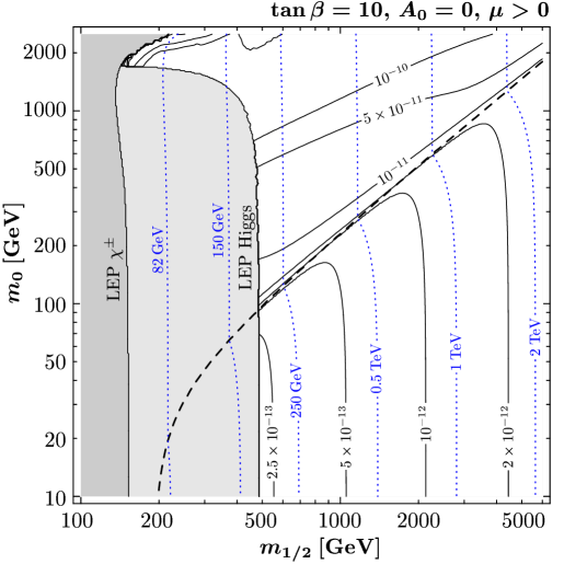
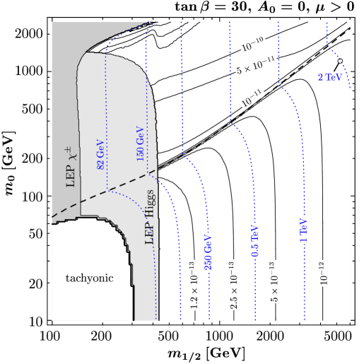
In Fig. 4.3 the solid (black) and dotted (blue) lines show respectively contours of and in the plane for , , (left panel) and (right panel). Above (below) the dashed line, (). The medium gray and the light gray regions at small are excluded respectively by the mass bounds and from chargino and Higgs searches at LEP [32]. The leftmost dotted (blue) line indicates the LEP bound [32]. For , tachyonic sfermions occur in the low-energy spectrum at points in the white corner labeled as “tachyonic.” For those scans we employ the computer program SuSpect 2.34 [161] to calculate the low-energy spectrum of the superparticles and the Higgs bosons.121212In this section, we have used the following values: , , , and . Assuming a standard cosmological history, the yield is obtained from the values provided by the computer program micrOMEGAs 1.3.7 [162, 163].
The contours shown in Fig. 4.3 are independent of and . Therefore, they can be used to interpret the results shown in the figures below. Note the sensitivity of both and on . By going from to , decreases by about a factor of two at points that are not in the vicinity of the dashed line, i.e., that are outside of the – coannihilation region. While becomes somewhat smaller by increasing to 30, the dependence of is negligible.
Let us now explore the parameter space in which the relic gravitino density matches the observed dark matter density (3.14),
| (4.14) |
Now, and appear in addition to the traditional CMSSM parameters. We focus on since the soft SUSY breaking parameters of the CMSSM are usually assumed to result from gravity-mediated SUSY breaking. However, we do not restrict our study to fixed relations between and the soft SUSY breaking parameters such as the ones suggested, for example, by the Polonyi model.
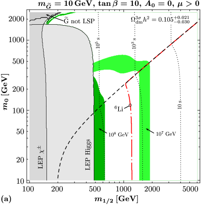
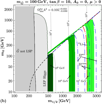
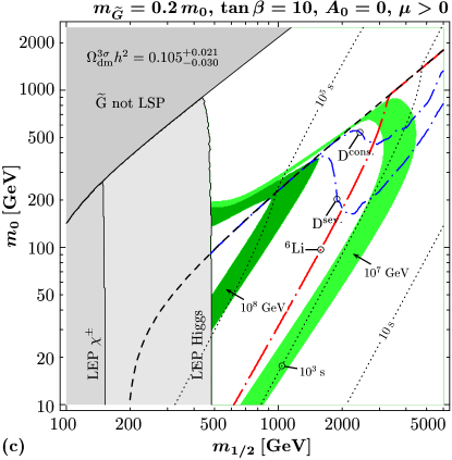
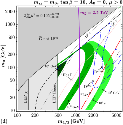
In Fig. 4.4 the light, medium, and dark shaded (green) bands show the regions that satisfy the upper limit (4.14) for , , and , respectively, where , , . The four panels are obtained for the choices (a) , (b) , (c) , and (d) . In the dark-gray region, the gravitino is not the LSP. The regions excluded by the chargino and Higgs mass bounds and the line indicating are identical to the ones shown in the upper panel of Fig. 4.3. The dotted lines show contours of the NLSP lifetime (4.4). For the NLSP, we calculate from the expressions given in Sec. IIC of Ref. [141].
The contours in Fig. 4.4 illustrate that the NLSP decays during/after BBN. Successful BBN predictions therefore imply cosmological constraints on , , and [141, 156, 137, 139]. Indeed, as stressed before, it has been found that the considered NLSP region is completely disfavored for by constraints from late electromagnetic and hadronic energy injection [141, 156, 137, 145]. In the NLSP region, the constraints from electromagnetic and hadronic energy release are important but far less severe than in the NLSP case.
Including the constraints from the bound-state effects this picture changes. As we have already seen in the previous section, in most of the NLSP parameter space, the bounds from the catalysis of and can be much more severe than the ones from late energy injection. We incorporate the -dependent CBBN constraint on from Fig. 4.2 which is shown in Fig. 4.4 by the long dash-dotted (red) line. The -NLSP parameter space to the left of this line is excluded.
We thereby update our figures presented in the published work [1]. In those figures, the output was taken from the work [79] which provided the initial estimate on the efficiency of the catalyzed production. Meanwhile, the dedicated quantum-three-body calculation [84] became available which lead to a reduction of the -factor of (2.40) by roughly one order in magnitude. As discussed in Chapter 2, we have incorporated this state-of-the-art result together with other improvements in our Boltzmann network equation.
In the lifetime region which is unconstrained by CBBN only the constraint from deuterium on the hadronic energy release becomes important. Following the approach explained in Sec. 4.1, we incorporate the constraint on hadronic energy release for D. In Fig. 4.4 these are shown by the short-dash-dotted (blue) lines. The D constraint disfavors the region between the corresponding lines in panel (b) and the region above the corresponding lines in panels (c) and (d). In panel (a) the D constraint does not appear. In addition, for orientation, in panel (d) we also include the electromagnetic constraint as a thin (pink) line and show the gluino mass contour which is a near to vertical thick (violet) line.
Indeed, one finds in each panel of Fig. 4.4 that the highest value allowed by the considered BBN constraints is about . The bands obtained for are located completely within the region disfavored by the 6Li bound. In previous gravitino dark matter studies within the CMSSM that did not take into account bound-state effects on the primordial 6Li abundance, much higher temperatures of up to about were believed to be allowed [156, 137, 119].
The constraint remains if we consider larger values of . This is demonstrated in Fig. 4.5 for , , , and (a) and (b) .
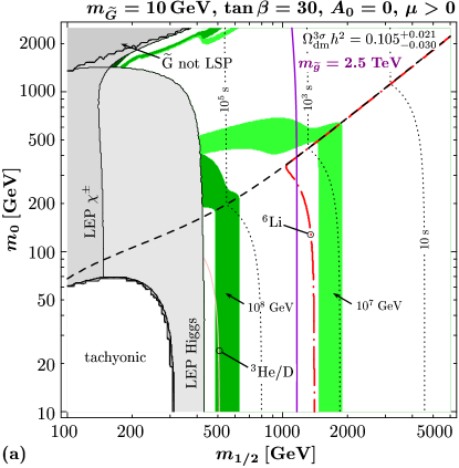
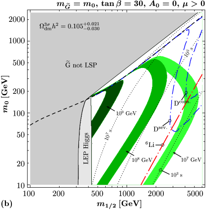
The shadings (colors) and line styles are identical to the ones in Fig. 4.4.
Let us comment on the dependence of the considered BBN constraints on the assumed primordial abundances of D and 6Li. As can be seen in Figs. 4.4 and 4.5, the constraint from late hadronic energy release is quite sensitive on the assumed primordial D abundance. In contrast, even if we relax the restrictive 6Li bound on by two orders of magnitude, we still find . For example, the 6Li constraint relaxed in this way would appear in Fig. 4.4 (b) as an almost vertical line slightly above .
- Limit on
-
The limit (4.11) emerges since scales with [see Fig. 4.3] and since is fixed once and are specified. The choice in Fig. 4.4 (a) and Fig. 4.5 (a) allows for an immediate comparison of the exemplary CMSSM scenarios with (4.11). Only in the vicinity of the dashed line, i.e., in the – coannihilation region, the position of the constraint approaches its conservative lower limit on . This is because becomes heavier for larger which shortens for fixed . Contrariwise, the splitting between the actual position of the constraint and (4.11) is larger for smaller . This is slightly more pronounced in Fig. 4.5 (a) than in Fig. 4.4 (a) and results from the fact that the increase in leads to a decrease in so that becomes larger for fixed .
That the lower limit (4.11) can imply high values of the superparticle masses is illustrated by the vertical (violet) lines in Figs. 4.4 (d) and 4.5 (a) which show the gluino mass contour . In this regard, also note that the mass of the lighter stop is in those NLSP regions with . Since there the gaugino mass parameter sets the scale for the low energy superparticle spectrum, depending on , the bound (4.11) implies high values of the superparticle masses which can be associated with a mass range that will be difficult to probe at the LHC.
- Limit on
-
The limit (4.13) relies on thermal gravitino production only, . Thus the upper limit on becomes more stringent by taking into account. In Figs. 4.4 (d) and 4.5 (b) we have fixed . Thereby, the non-thermal production (4.2) becomes more important for larger values of . In addition, takes on its maximum at a given in the – coannihilation region. This leads to the bending of the bands (4.14) towards lower . This indicates that (4.13) indeed seems to provide a good estimate.
While the constraint is found for each of the considered relations, one cannot use the 6Li bound to set bounds on without insights into . The 6Li (and similarly the ) bound disappears for [79] which is possible even for provided is sufficiently small; see (4.4). However, the constraints on become more severe towards small as is shown in Fig. 3.3. Thus, the constraint cannot be evaded by lowering provided . An upper limit on of can be problematic for inflation models and baryogenesis scenarios. This finding can thus be important for our understanding of the thermal history of the Universe.
4.2.4 Late-time entropy production
The constraints shown above are applicable for a standard thermal history during the radiation-dominated epoch. Such a standard cosmological evolution may, e.g., be accomplished by considering only a minimal framework such as the MSSM.131313Even inflation seems to be feasible within the MSSM with the inflaton being a gauge invariant combination of squark and slepton fields [164]. Strictly speaking, however, neutrinos do not obtain masses within this framework which are needed to explain the observed neutrino oscillations [165].
On the other hand, focusing on a gravitino LSP we also explicitly consider the gravity sector. For example, it is well known that supergravity and string theories generically suffer from the appearance of scalar fields which can give rise to “cosmological moduli problems” [166, 167, 168]. Typically, the interaction of such an exotic (eventually) massive field to the MSSM sector is suppressed by a high-energy scale such as or . The problem arises because easily drops out (or never has reached) thermal equilibrium.
For a massive particle species which is in equilibrium, the energy density becomes exponentially suppressed once the temperature drops below its mass. However, if is frozen-out, starts to scale as so that, eventually, the energy density in dominates over the one in radiation. Thus, if lives sufficiently long, it is possible that a substantial amount of entropy is released in its out-of-equilibrium decay.141414 Other entropy production events after inflation are, e.g., Q-ball decays; cf. [169] and references therein. Gravitino dark matter scenarios with late-time entropy production have been considered previously for gauge-mediated SUSY breaking where [170, 171, 172, 173, 174]. Since an entropy release tends to erase any pre-existing quantity which itself has originated from a non-equilibrium process—such as —this can be problematic. Moreover, additional unwanted relics can be produced in the decay of leading, e.g., to too much dark matter. However, as we shall see in the following, entropy production can also have a positive effect [175].
The change in entropy per comoving volume is found from the “heat added” in the decay, [176]. The associated evolution of the entropy per comoving volume is thus described by
| (4.15) |
We have already indicated by the chosen notation that the situation is somewhat similar to that at the end of inflation. Thus, we can solve (4.15) by simultaneously considering the Boltzmann equation for in the form (3.11b) together with the Friedmann equation which governs the evolution of the scale factor of the Universe; denotes the decay width of .
From the discussion of Sec. 3.3.1 we know that the temperature after the decay can be expressed in terms of ,
| (4.16) |
which satisfies . Note that primordial nucleosynthesis imposes a lower limit on this temperature. It mainly emerges from the fact that a re-thermalization of all the three neutrino species after the reheating process does not happen instantaneously. Insufficient thermalization affects the Hubble rate, thereby the freeze-out value, and thus the output in BBN [see Sec. 1.3]. The bounds derived in [177, 178, 179, 180] are in the range
| (4.17) |
In the upper panel of Fig. 4.6 we show the evolution of , , and for two exemplary scenarios respecting (4.17). The scale factor is normalized by151515Giving the dimension of a length makes the radial coordinate in the Friedmann-Robertson-Walker metric dimensionless. and the temperature dependence of is taken into account as determined in [28]. For and , increases by a factor of as shown by the corresponding solid line. For and , increases by a factor of as shown by the corresponding dotted (blue) line.
The lower panel of Fig. 4.6 shows the associated evolution of the photon temperature for the case . As long as the comoving entropy is conserved, . This causes to decrease slightly less slowly than during the quark-hadron transition at which we have assumed to be adiabatic [181]. As already encountered in Sec. 3.3.1, the temperature scales with during entropy production, i.e., during reheating, the temperature does not increase but rather drops less slowly [176]. Below the Universe again expands as a radiation-dominated one.
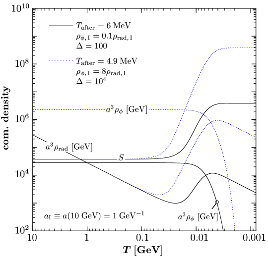
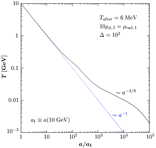
In the following, we restrict our study of entropy production at late times, , so that the thermal production of gravitinos is not affected. We assume that the production of gravitinos and NLSPs in the entropy producing event, such as the direct production in decays of , is negligible.161616Note however, if kinematically allowed, a field will also typically decay into SUSY particles [182, 183, 122]. Thus, the constraints discussed below shall therefore be considered as conservative/optimistic bounds. Moreover, in this section, we focus on scenarios in which the decoupling of the NLSP is not or at most marginally affected by entropy production, i.e., either or for . Note that the latter condition excludes the event shown in Fig. 4.6 with ; see, however, Sec. 4.2.5. Thus, the thermally produced gravitino yield and—in the case of entropy production after NLSP decoupling—also the non-thermally produced gravitino yield are diluted:
| (4.18) |
In the case of late-time entropy production before the decoupling of the NLSP, we parameterize this by writing
| (4.19) |
In this case, and thereby and the BBN constraints remain unaffected.
Conversely, in the case of late-time entropy production after the decoupling of the NLSP (and before BBN) both, and , are reduced:
| (4.20) |
Accordingly, and become smaller and the BBN constraints can be relaxed.
In Fig. 4.7
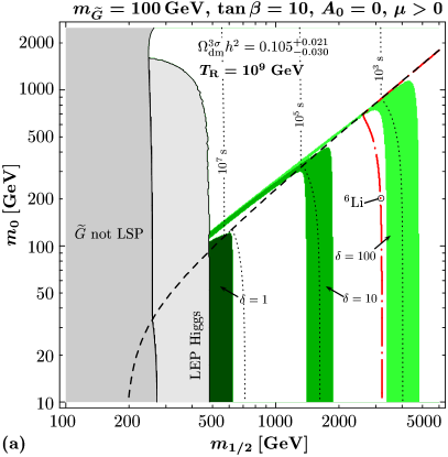
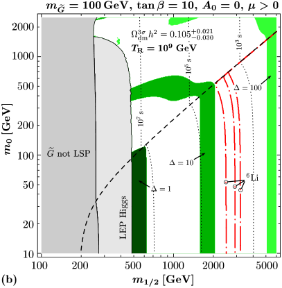
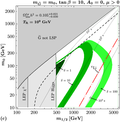
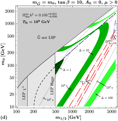
we show how late-time entropy production before (left) and after (right) NLSP decoupling affects the 6Li constraint and the region in which for . The planes are considered for , , , (upper panels) and (lower panels). The dark shaded (dark green) region is obtained without late time entropy production, . The medium and light shaded (medium and light green) bands are obtained with a dilution of () by () and (), respectively. The dot-dashed (red) line illustrates that the 6Li bound is independent of , as shown in the panels on the left-hand side, and becomes weaker (i.e., moves to the left) with increasing , as shown in the panels on the right-hand side. Other curves and regions are identical to the ones in the corresponding panels of Fig. 4.4. Note that we do not show the D constraint on late hadronic energy injection since it is not sensitive to and vanishes already for ; an exception is the severe D constraint which still appears for in panel (a). BBN constraints on NLSP scenarios with entropy production after NLSP decoupling will be studied elsewhere.
Comparing panels (b) and (d) of Fig. 4.4 with panels (a) and (c) in Fig. 4.7, we find that a dilution factor of () relaxes the bound by a factor of 10 (100). Since the BBN constraints are unaffected by , the cosmologically disfavored range of NLSP masses cannot be relaxed. With the dilution after NLSP decoupling, the relaxation of the constraints is more pronounced. Here also the cosmologically disfavored range of NLSP masses can be relaxed [175]. However, as can be seen in panels (b) and (d) of Fig. 4.7, the 6Li bound is persistent. With a dilution factor of , large regions of the plane remain cosmologically disfavored. For even larger factors of , however, the 6Li bound can be evaded as will be shown explicitly below.
Figure 4.7 shows that inflation models predicting, for example, become allowed in the CMSSM with gravitino dark matter for . Here it is not necessary to have late-time entropy production in the somewhat narrow window between NLSP decoupling and BBN. This is different for the viability of thermal leptogenesis in the considered scenarios where .
4.2.5 Viability of thermal leptogenesis
The constraint obtained in the considered CMSSM scenarios for a standard cosmological history strongly disfavors thermal leptogenesis. However, if entropy is released after NLSP decoupling, a dilution factor of can render thermal leptogenesis viable for .
Thermal leptogenesis—in its simplest form, with hierarchical heavy right-handed Majorana neutrinos —usually requires [134, 135, 184, 185].171717Right-handed (heavy) neutrinos (and their superpartners) are not part of the (C)MSSM. Again, this section contains an updated discussion of the published work [1]; see Sec. 4.2.3. However, late-time entropy production dilutes the baryon asymmetry which is generated well before NLSP decoupling,
| (4.21) |
Therefore, the baryon asymmetry before entropy production must be larger by a factor of in order to compensate for the dilution. For , this can be achieved in the case of hierarchical neutrinos for , as can be seen in Fig. 7 (a) of Ref. [186] and in Fig. 2 of Ref. [187]. Here, is the mass of the lightest among the heavy right-handed Majorana neutrinos.
That it is indeed possible to produce such a large amount of entropy in the narrow time window between NLSP decoupling an BBN, we show in Fig. 4.6 a scenario in which a dilution factor of even is generated in the out-of-equilibrium decay of a heavy particle [dotted (blue) lines]. However, because of , the Hubble rate is already enhanced already during the decoupling phase of the NLSP. This leads to an increase of and . In the results shown below, we indeed account for this by using a modified version of the micrOMEGAs code. Thereby, the contours shown in Fig. 4.3 do not apply in this section. After entropy production, the net effect is still a significant reduction of —provided that does not decay into SUSY particles.
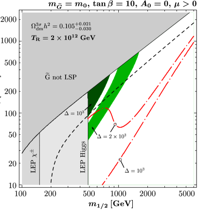
In Fig. 4.8 we consider now two concrete scenarios with as initial condition and with and corresponding to the respective reheating temperatures and . We choose the -plane with , , , and . Here the shaded (green) bands indicate the region in which for and (dark) and (medium). In addition, the corresponding evolution of the 6Li bound is shown by the dot-dashed (red) lines. The regions in the -NLSP region above the curves remain cosmologically disfavored. The gray regions are identical to the ones in Fig. 4.5.
We find that the 6Li bound can indeed be evaded for . Gravitino dark matter scenarios with successful thermal leptogenesis in the NLSP region are located on the light-shaded (light green) band. As can be seen in Fig. 4.8, the NLSP region with where (cf. Fig. 4.3), is no longer disfavored by the 6Li bound provided . Such scenarios are particularly promising since the long-lived NLSP could provide striking signatures of gravitino dark matter at future colliders [154, 188, 189, 190, 191].
Finally, let us remark that the exact value of the actual amount of entropy required is model dependent. Though we have accounted for the fact that the presence of the energy density during NLSP decoupling can affect , we have neglected a possible branching ratio of the decays into and/or gravitinos. Moreover, such a scenario is—of course—fine-tuned since entropy has to be released in a very narrow time window. However, with our improved treatment of the CBBN yield of it becomes slightly easier (when compared to [1]) to circumvent the stringent bound.181818The value is now in the region provided by the more recent Ref. [84] in which also our employed CBBN rate for production was obtained. The authors, however, only use the Saha approximation for the bound state abundance; see Sec. 2.3. This is indicated by the fact that we were able to allow for an increased NLSP decoupling yield by choosing which lead to the generous choice of . Since we have not provided explicitly a model for we understand the results presented in this section as a proof-of-concept study that a non-standard cosmological evolution can evade even the most stringent of all BBN constraints while still allowing for successful leptogenesis.
Part III The long-lived stau as a thermal relic
Chapter 5 Thermal relic stau abundances
In Part I of this thesis we worked out the effects which a long-lived electrically charged massive particle species has on the predictions of primordial nucleosynthesis. In Part II we then considered concrete realizations of in gravitino dark matter scenarios in which is the lightest Standard Model superpartner. There, a central parameter in the investigation is the abundance of during/after BBN. For a standard thermal history it is determined by and by its thermal freeze-out value which we shall call in the following; recall that is the total stau number density normalized to the entropy density prior to its decay .
In particular, we saw that (i) governs the non-thermally produced relic density (4.2) of gravitino dark matter that originates from decays, (ii) controls the hadronic and electromagnetic BBN constraints by quantifying the total energy density which is eventually be released in the decay and (iii) parameterizes the abundance of recombination partners with the light elements leading to the catalysis of BBN.
Importantly, the points (i)-(iii) have in common that they give rise to upper limits on : (i) For example, for and a thermally produced gravitino density (), one finds from (4.14) (); see also Fig. 13 of [139]. (ii) The BBN constraints on hadronic and electromagnetic energy release can be as restrictive as (); cf. Fig. 12 of [139] and Figs. 14 and 15 of [130]. (iii) Catalyzed production of 9Be (and 6Li) imposes restrictive upper limits of ( – for ; see Fig. 2.9.
In Chapter 4 we have either made use of representative values (4.1) of or performed exemplary CMSSM parameter scans which gave us , e.g., for fixed values of and . In this chapter we now calculate by taking into account the complete set of stau annihilation channels in the MSSM with real parameters for SUSY spectra for which sparticle coannihilation is negligible. Using our own code for the computation of the resulting thermal relic stau abundance , we examine explicitly (i) the effect of left–right mixing of the lighter stau, (ii) the effect of large stau–Higgs couplings, and (iii) stau annihilation at the resonance of the heavy CP-even Higgs boson . We consider both the “phenomenological MSSM” (pMSSM) (see, e.g., [161]) in which the soft SUSY breaking parameters can be set at the weak scale, and the CMSSM.
Within the framework of the pMSSM, we show examples in which can be well below . Even within the CMSSM, we encounter regions with exceptionally small values of . We stress that the results in the following are independent on the nature of the LSP. However, we discuss the implications of these findings for the gravitino-stau scenario.111For simplicity, we call the parameter region in which the -NLSP region in the following. We also address the viability of a – asymmetry. The key quantities for the significant reduction could be probed at both the LHC and the ILC.
The work presented in this chapter is based on the publication [5]. A calculation of the thermal relic abundance of long-lived staus has also been part of a detailed study [36] which focuses on gauge interactions and on the effect of Sommerfeld enhancement. In contrast, the most striking findings of our study—in which Sommerfeld enhancement is not taken into account—are related to the Higgs sector of the MSSM.
We also remark that our work has some overlap with [192] which appeared as [5] was being finalized. Whereas [192] focuses on the potential suppression in due to enhanced annihilation into the lighter Higgs final state, our work provides an investigation of stau decoupling based on a complete set of annihilation channels. Thereby, we also study enhanced stau annihilation into heavier Higgs final states and consider annihilation at the heavy Higgs resonance.
The outline of this chapter is as follows. In the next section we review basic properties of the staus to introduce our notations and conventions for the stau mixing angle. Section 5.2 explains the way in which we calculate and provides the complete list of stau annihilation channels. In Sec. 5.3 we analyze the dependence of the most relevant stau annihilation channels on the stau mixing angle. Effects of large stau–Higgs couplings and stau annihilation at the resonance are studied in Sects. 5.4 and 5.5, respectively. The viability of a – asymmetry is addressed in Sec. 5.6. In Sec. 5.7 we present exemplary parameter scans within the CMSSM that exhibit exceptionally small values. Potential collider phenomenology of the parameter regions associated with those exceptional relic abundances and potential implications for gravitino dark matter scenarios are discussed in Sects. 5.8 and 5.9, respectively.
5.1 Stau mixing and mass eigenstates
In this section we review some basic properties of the stau to set the notation. In absence of inter-generational mixing, the stau mass-squared matrix in the basis of the gauge eigenstates reads
| (5.1) |
with
| (5.2) | |||||
| (5.3) | |||||
| (5.4) |
Here, and are the soft SUSY breaking masses, is the trilinear coupling, is the Higgs-higgsino mass parameter, and denotes the ratio of the two Higgs vacuum expectation values. In this work we restrict ourselves to the MSSM with real parameters. Then so that the mass eigenstates and are related to and by means of an orthogonal transformation
| (5.5) |
with denoting the stau mixing angle. Imposing the mass ordering and choosing , the mixing angle can be inferred from the elements of ,
| (5.6) |
where the sign of the second relation determines the quadrant of . In the first relation, we have introduced . In particular, corresponds to a purely right-handed stau, , whereas maximal mixing occurs for and . The physical stau masses are then given by
| (5.7) |
from which we see that an increase of leads to a reduction of .
5.2 Calculation of the thermal relic stau abundance
We have undertaken the effort to set up our own full-fledged relic abundance calculation. Let us in the following give a description of our approach to compute the stau yield . Throughout this work we assume a standard cosmological history with a temperature of the primordial plasma above the stau decoupling temperature so that the lighter stau was once in thermal equilibrium. Then, the total stau yield is found by solving the Boltzmann equation (1.9) with Using the Maxwell–Boltzmann approximation, the stau equilibrium yield is given by
| (5.8) |
and the thermally averaged annihilation cross section by [28]
| (5.9) |
where is the modified Bessel function of order and .
Note that contains all the information from the particle physics side. It is obtained by computing the total stau-annihilation cross section,
| (5.10) |
where the sum for the annihilation of pairs222Counting wise we distinguish between and the conjugate process . In absence of CP violation in the SUSY sector, their cross sections agree so that we can solve a single Boltzmann equation (1.9) for obtaining . has to be taken over all final states . The factor is convention but gives (1.9) its familiar form. The complete list of annihilation processes in the MSSM with real parameters—save for coannihilation processes—is given in Table 5.1.333For a purely right-handed stau , the stau annihilation channels and associated cross sections have already been presented in Ref. [193] in the context of - coannihilation. In addition, this table shows all possible particle exchanges, where , , and are the Mandelstam variables which denote the respective channel. A number of annihilation processes proceeds also via a four-point vertex. Those are marked in the column named “contact.” Already by mere optical inspection, we immediately see that the Higgs sector plays potentially an important role in the determination of the stau yield .
| final state | -channel | -channel | contact | |
|---|---|---|---|---|
| — | — | |||
| final state † | -channel | -channel | contact | |
| , | — | — | ||
| — | ||||
| , | — | — | ||
| — | ||||
| — | — | |||
| — | ||||
| — | — | |||
| — | ||||
| — | ||||
| — | ||||
| — | ||||
| † | ||||
For all channels in Table 5.1, we generate Fortran code for the squared matrix elements by using the computer algebra packages FeynArts 5.4 [194, 195] and FormCalc 5.3 [196, 197]. For a chosen point in the SUSY parameter space, we then compute the radiatively corrected superparticle spectrum by running the spectrum generator SuSpect 2.40 [161]. Its output allows us to set all SUSY parameters so that we can compute the total cross section given by (5.10) and subsequently the thermally averaged cross section (5.9). Numerically, the computation of (5.9) is the most demanding part in the relic abundance calculation. In particular, we take special care about the following cases:
-
•
-resonance: Resonant stau annihilation via exchange is one of the central points in this part. In the generation of the matrix elements, we have therefore included the total -width in the respective -channel propagators.
-
•
Propagator poles: A diverging -channel propagator can be encountered when a production threshold is met. We overcome this problem by including a “sparticle-width” of in the respective propagators in the vicinity of dangerous thresholds. A particularly interesting example with a diverging -channel propagator is given by the process if is fulfilled since then the -exchange in the -channels of other processes is resonant simultaneously.
-
•
Bessel functions: The Bessel functions in (5.8) and (5.9) exhibit an exponential behavior for large arguments [68]
(5.11) For small temperatures , the arguments of and in (5.9) become large simultaneously. Therefore, in order to ensure numerical stability, we expand the Bessel functions in (5.9) for as in (5.11) and cancel the exponents analytically.
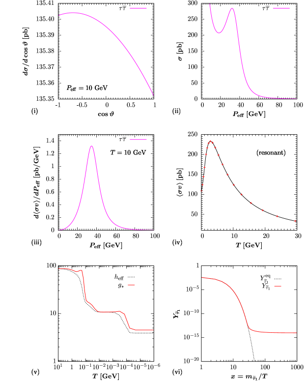
We find the starting point for the numerical integration of (1.9) by solving [163]
| (5.12) |
where is given by (1.10). marks the point at which the stau starts to decouple chemically from the background plasma, with [163] chosen in our code. Since we use a globally adaptive Gaussian integration routine to calculate (5.9), the computation of is time-demanding. Therefore, we evaluate (5.9) on a grid of different temperatures and use cubic spline interpolation to obtain values in between. We then solve the Boltzmann equation (1.9) by numerical integration from to zero. There, we fully take into the account the temperature dependence of and by interpolating the respective tabulated values provided as part of the relic density code DarkSUSY 4.00 [33]. The freeze out temperature can then be defined by where is given by [163]. For , residual annihilations will further reduce so that we refer to the decoupling yield as the quantity at the endpoint of integration. As already pointed out in the introduction, for simplicity, we call this yield . Moreover, we will quantify in terms of and in particular in terms of . We have also schematically depicted the approach to in Fig. 5.1 for an exemplary scenario (which gives rise to resonant stau annihilation. See the figure caption for details.)
Note that we have additionally modified the FeynArts MSSM model file for the generation of the matrix elements in two ways: The first version, which we use throughout Sects. 5.3–5.5, allows us to set all –Higgs and all trilinear Higgs couplings by using the computer tool FeynHiggs 2.6.3 [198]; see also Sects. 5.4 and 5.5. The second version allows for a direct comparison with the existing computer code micrOMEGAs 2.0.6 [162, 163, 199]. We have transcribed their routine [200] for the computation of the running quark masses to Fortran, adopted all –Higgs couplings, and modified all Higgs-self couplings of our matrix elements to match with their implemented version of the MSSM [201]. Using this second version, we find perfect agreement between our codes.444For our computation we use the Standard Model parameters , , , , and . Since micrOMEGAs has hard-coded from which it computes using the on-shell relation with , we follow their convention to allow for a better comparison of our results with micrOMEGAs.
5.3 Dependence of stau annihilation on the stau mixing angle
In order to isolate the distinct features of the different annihilation processes we need to have full control over the superparticle mass spectrum. Therefore, in the following, we will not rely on any constrained model (such as the CMSSM) where the soft-SUSY breaking parameters are subject to stringent boundary conditions at some high scale (such as ). In those models, the mass spectrum is found only after renormalization group (RG) evolution from the high scale down to the electroweak scale. Instead, we choose to work in the framework of the “phenomenological MSSM” (pMSSM), see, e.g., [161]. There, all soft-SUSY breaking parameters can be set at the scale of electroweak symmetry breaking—a low scale—which we fix to . In particular, one can also trade the Higgs mass-squared parameters and against and the pseudoscalar Higgs boson mass .555Though the advocated procedure may require fine-tuning in the electroweak symmetry breaking conditions, it conveniently provides us with running parameters at the scale of stau annihilation. Choosing as an input parameter is very convenient for two reasons: First, together with the specification of the gaugino masses we have control over the gaugino/higgsino mixture of the neutralinos . Second, enters directly into the stau-Higgs couplings, whose importance will become clear in the next section. Furthermore, in the following, we choose to set all soft-SUSY breaking scalar masses (apart from and ) to a common value . Thereby, we essentially decouple all sfermions which are not of interest for us. This ensures also that we never enter accidentally any coannihilation regime. Finally, for simplicity, we set also all trilinear parameters to a common value . Given , , and , and thereby , we can then fix and to arbitrary values by adjusting and in Eqs. (5.6) and (5.7).
In the following, we will focus on two distinct regions of the SUSY parameter space. In the beginning, we will choose to be very large . This corresponds to the decoupling limit of the MSSM where the following (tree-level) relations hold [202]
| (5.13) | ||||
| (5.14) |
Therefore, up to corrections so that any of the stau annihilation channels into heavy Higgs bosons is kinematically blocked. Furthermore, up to corrections implies that the coupling () becomes very small so that we loose the -exchanges in the stau annihilation channels with a final state. At the same time, the light Higgs boson takes on its Standard Model value for the coupling. Complementary to that we will consider also regions of the SUSY parameter space with smaller , e.g., in the next section, where we will put a stronger focus on the Higgs sector and its connection to .
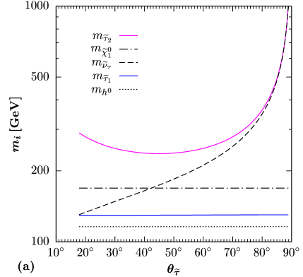
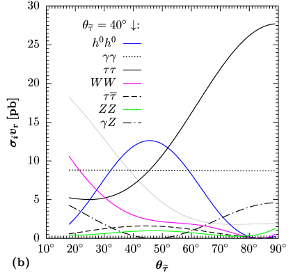
In Fig. 5.2a we show the -dependence of the masses of the heavier stau, , (curved solid line) and the tau-sneutrino, , (dashed line) for fixed and the input parameters , , and . Because of SU(2) gauge invariance, sets also the soft-breaking mass for the tau-sneutrino hence approximately so that becomes lighter than for ( is negative in that region). In addition, we plot the masses of the lightest neutralino, (dash-dotted line), the lighter stau, (horizontal solid line), and the lightest Higgs, (dotted line). We note in passing that may deviate slightly from its anticipated input value due to radiative corrections. We then correct for this by an adjustment of so that we indeed ensure to be constant.
In Fig. 5.2b we plot the dominant stau annihilation cross sections times the relative (non-relativistic) velocity in the center-of-mass frame of the incoming staus, , for the same parameters as in Fig. 5.2a. Owing to an (approximate) Maxwell-Boltzmann distribution of the stau velocity, , we choose as a representative value.666This value is actually at the somewhat lower end, given and . However, depends only weakly on , and the thermally averaged will be shown in the upcoming figures. The curves show the annihilation channels with the following final states: , , , , , , (at , from top to bottom). All channels except show a strong dependence on . The () channel peaks at —a feature which we will discuss in detail in Sec. 5.4. For the channel, the overall size of the cross section is governed by since this channel proceeds only via -channel exchanges of neutralinos. Our chosen input values lead to a bino-like neutralino, , and drops for an increasingly ‘left-handed’ stau. (For comparison, the thin gray line shows for the case of a wino-like lightest neutralino, , of similar mass, , as obtained by changing the gaugino mass input parameters to .) The annihilation into a pair becomes important for an increasing component in , i.e., towards smaller , since the -channel exchange with the tau-sneutrino opens up; the () coupling is proportional to (). The modulation of the channel can be understood by considering the structure of the coupling . Note that the first two terms practically cancel out. For stau annihilation into a pair there is an additional contribution from -exchange with the respective coupling . Having discussed the dominant annihilation channels in a simple manner, we also warn the reader that interferences between the different Feynman diagrams of a given channel may well lead to a counter-intuitive behavior. In this regard, see Ref. [36] for a thorough discussion of annihilation into vector bosons. For the limiting case of a purely ‘right-handed’ stau, (), we recover the relative importance of the annihilation cross sections into , , , and with bino -channel exchange found in Ref. [31].
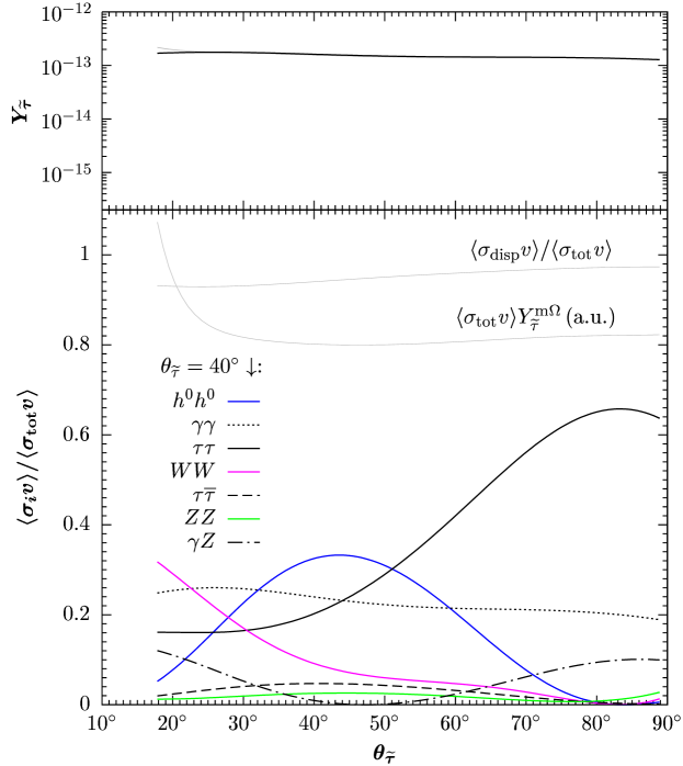
Figure 5.3 shows the -dependence of (upper panel) and of the relative importance of the dominant thermally averaged cross sections, , at (lower panel) for the same input parameters as in Fig. 5.2. The lines in the lower panel are associated with the same dominant annihilation channels as in Fig. 5.2b. In addition, the relative importance of the sum of the displayed cross sections, , (thin line, as labeled) is shown to demonstrate that the displayed channels constitute indeed (up to at most about ) the dominant part of for the chosen set of input parameters. In the upper panel, the total stau decoupling yield obtained with our own relic abundance calculation is shown by the thick line and the one computed with micrOMEGAs, , by the thin gray line. For , both curves start to deviate from each other since one enters the – coannihilation region in which the stau decoupling yield increases. This coannihilation effect leads also to the rise of the thin gray line that shows in arbitrary units (a.u.) in the lower panel. Note that the same line illustrates for , where the result of our relic abundance calculation agrees with . Interestingly, for the given input parameters, is not overly affected by the variation in in this region, which reflects the fact that and thereby vary by less than a factor of about at the relevant time of decoupling. In the next sections, we will demonstrate that this picture changes significantly for certain other choices of the input parameters.
5.4 Effects of large stau-Higgs couplings
Owing to the scalar nature of the stau, there exists a remarkable difference between the standard neutralino decoupling and the scenario in which the long-lived stau freezes out from the primordial plasma. For the neutralino LSP, the parameter enters into the annihilation cross sections only indirectly by influencing the gaugino/higgsino mixture of . This stands in strong contrast to the case in which a scalar particle is the lightest Standard Model superpartner: the sfermions couple directly to dimensionful parameters of the theory, namely, the trilinear couplings and the Higgs-higgsino mass parameter . The corresponding operators in the MSSM Lagrangian always contain a Higgs field. In particular, the stau–Higgs couplings are given by
| (5.15) |
with . We have pulled out the factor so that the ‘reduced’ couplings among the gauge eigenstates and are given by [203]
| (5.16) | ||||
| (5.17) |
where can be obtained from (5.16) upon the replacement . Whenever convenient, we use the shorthand notation , , and . The parameters and only appear off-diagonal and they are multiplied with the associated fermion mass, the tau mass .
Using , one obtains the couplings of the mass eigenstates and . In this regard, it is important to note that the coupling of the CP-odd Higgs boson to the lighter stau vanishes, . Therefore, we have not listed the process in Table 5.1. By the same token, there is also no -channel exchange of in any of the annihilation channels. Note that this statement remains valid even after the inclusion of radiative corrections: There is no induced mixing between and in absence of CP-violating effects in the SUSY sector.
Let us now turn to the probably most interesting couplings in the context of annihilation, namely, the ones of the lighter stau to and . The ‘reduced’ coupling reads
| (5.18) |
This is a complicated expression. However, if we choose to be large, , we can simplify (5.18) by using [cf. (5.14)],
| (5.19) |
Thereby, we make an interesting observation: In the decoupling limit (DL), the coupling becomes proportional to the left–right entry of the stau mass-squared matrix (5.1) and to . Therefore, it comes as no surprise that the annihilation cross section into peaks at —the point of maximal - mixing—as can be seen, e.g., in Fig. 5.2b. Analogously, one finds that the coupling is proportional to in the decoupling limit. Complementary, the couplings exhibit in this limit the same combination of , , and as their counterparts but those terms are now multiplied by instead of .
After the above discussion, it is clear that there exists the possibility to enhance the total stau annihilation cross section —and thereby to decrease —by choosing a proper combination of large , , and . In the remainder of this section, we will explore this possibility for two exemplary pMSSM scenarios.
Before proceeding let us make some technical comments. Large values of the previously mentioned parameters may well lead to large radiative corrections.777In this context, note that we introduce a large – splitting when choosing . In order to arrive at a proper loop-improved tree-level result, we re-evaluate the entire Higgs sector using FeynHiggs. In particular, we have modified our generated matrix elements in a way that allows us to set all trilinear Higgs couplings to their loop-corrected values.888The author grateful to T. Plehn and M. Rauch for providing us, for cross-checking, with their implementation of a Fortran routine which calculates the Higgs self-couplings using the effective potential approach [204]. Note that this goes well beyond a simple prescription. Only then, we mostly find better agreement of our cross sections for stau annihilation into two Higgses with the ones computed by micrOMEGAs. The latter program uses CalcHEP [200] for the generation of the matrix elements. There, the trilinear Higgs self-couplings have been expressed in terms of , , and which effectively reabsorbs a bulk of the radiative corrections [201]. We therefore think that we do slightly better whenever we encounter some disagreement between the mentioned cross sections. Though the overall effect on is typically small, it can be at the level of (see below). Finally, it is well known that a large parameter may lead to charge/color breaking minima (CCB) in the scalar MSSM potential; see, e.g., Ref. [205]. SuSpect performs some basic checks which we take into account to make sure that we do not violate the constraints associated with CCB. We remark that our pMSSM scenarios are chosen such as to allow us to extract the important features of primordial stau annihilation in the most transparent way—without emphasis on naturalness considerations.
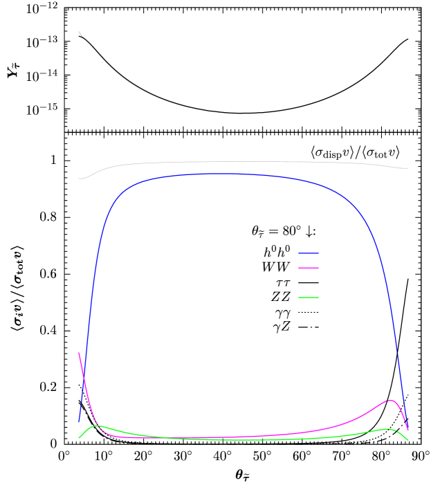
In Fig. 5.4 we demonstrate the effect associated with a large coupling by presenting the -dependence of (upper panel) and of the relative importance of the dominant thermally averaged cross sections, , at (lower panel) for the pMSSM scenario associated with , , , and . In this scenario, stays in the range and the lightest neutralino is bino-like with a mass of . Stau annihilation into heavy Higgses remains kinematically forbidden. The curves in the lower panel are associated with stau annihilation into , , , , , and (at , from top to bottom). As is evident, the annihilation into is enhanced already well before . At the peak position, for (no thermal average), which is still three orders of magnitude below the unitarity bound for inelastic s-wave annihilation, [206, 36]. Also the cross sections for stau annihilation into and are strongly enhanced towards since the -channel contribution of becomes very important. At their respective peak positions, and for . (Because of the dominance of the channel, the corresponding maxima do not show up in Fig. 5.4 where is shown.) By the same token, the cross sections of all (kinematically allowed) channels with a fermion-antifermion final state (e.g. )—which are subdominant in the scenario considered in Fig. 5.4—experience an enhancement for . In total, there is an enhancement of that delays the thermal freeze out of the staus significantly, i.e., for . As can be seen in the upper panel of Fig. 5.4, the decoupling yield is thereby reduced dramatically down to a minimum value of for maximal left–right mixing of the staus.
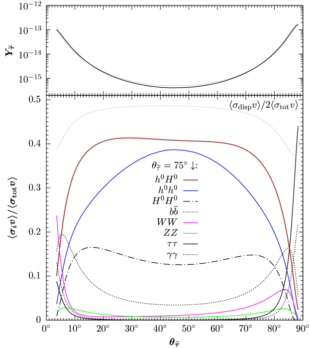
In the previous pMSSM examples, annihilation into final states containing heavy Higgs bosons is kinematically forbidden. We can allow for those channels by reducing the input value . Indeed, scenarios in which all Higgs bosons are very light in conjunction with large have been studied in the literature, see, e.g., [207, 208] and references therein. We thus consider now the following pMSSM scenario: , , , , and . In Fig. 5.5, the associated -dependence of and of at for the now dominant channels is shown in a similar way as in Fig. 5.4; only the relative importance of the sum of the displayed cross sections is scaled down by a factor of 1/2, , to allow for an optimized presentation of the single dominant channels. Throughout the considered range, the masses of both CP-even Higgs bosons are relatively light and remain rather constant: and . Here the dominant annihilation channels are associated with the following final states: , , , , , , , and (at , from top to bottom). As can be seen, stau annihilation into is now more dominant than the one into and also the channel becomes important, where each of those channels is indeed associated with an (absolute) annihilation cross section that peaks at . Also the annihilation into is significant—a process which we will discuss in detail in the following section. In this respect, one should stress that all processes with -channel exchange are here less suppressed by in the respective propagator than in the previously considered scenarios. Note that the asymmetry of of those dominant channels (, , , ) with respect to a reflection at is dominantly caused by the -dependent modulation of the channel. As in the pMSSM scenario considered in Fig. 5.4, there is again an significant enhancement of that delays the stau freeze out such that at . Thereby, the efficient annihilation into final state Higgses is accompanied by a significant drop in down to at as can be seen in Fig. 5.5. At this minimum, there is a disagreement between from our calculation of stau decoupling (solid line) and the micrOMEGAs result (thin gray line) which is a consequence of the different treatments of the Higgs sector described above.
Let us finally remark that the Higgs couplings to fermions and vector bosons as well as the Higgs self-couplings develop a strong dependence on once we leave the decoupling regime (); for a comprehensive review see, e.g., Ref. [209].999The Higgs sector is also particularly sensitive to the mixing in the stop sector. In the considered pMSSM scenarios, which corresponds to the “typical-mixing scenario” [210]. Changes in can therefore be accompanied by shifts in the relative importance of the corresponding annihilation cross sections. This underlines the fact that the details in the Higgs sector may very well be crucial for the determination of the relic abundance of a long-lived .
5.5 Resonant stau annihilation
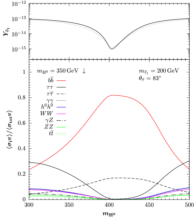
By inspection of Table 5.1 it becomes clear that primordial stau annihilation can also proceed resonantly via -channel exchange of the heavy CP-even Higgs boson for . While the LEP bound on the stau mass [32] forbids to become on-shell (, e.g., [209]), the -channel exchange of is absent101010Even in absence of SUSY-induced CP violation, resonant annihilation via -exchange may still proceed through - coannihilation. However, this scenario requires considerable fine-tuning in the stau mass-squared matrix since and have to be nearly degenerate. because of (see Sec. 5.4). Again, our choice to work in the framework of the pMSSM proves to be very helpful. Since the resonance occurs for , one runs quickly into the decoupling limit in which is governed by the input parameter according to the simple relation (5.13). This allows us to scan through the resonance easily.
Let us explore resonant stau annihilation by considering the exemplary pMSSM scenario associated with , (i.e., a mostly ‘right-handed’ ), , and , for which we vary (and thereby ) to scan through the resonance. Figure 5.6 shows the resulting -dependence of (upper panel) and of at for the dominant annihilation channels (lower panel). Those channels are now associated with the following final states: , , , , , , , , and (at , from top to bottom). In Table 5.1 all resonant channels can be identified. Close to the resonance condition , the most important processes are stau annihilation into and . This is because the couplings of those final state fermions to are enhanced: for , the coupling with [203]. The (broad) peak associated with the resonance111111Notice that we plot so that the actual shape of the resonance looks somewhat different. already builds up for . At zero relative velocity, this would be a region in which the resonance cannot occur. However, since is in kinetic equilibrium at the time of freeze out, resonant annihilation takes place already for [29]. For , the processes containing -channel exchange proceed with a slightly faster rate (if kinematically allowed). The impact of the resonance on the thermal freeze out and the resulting is substantial. Since the total width of is for in the considered pMSSM scenario, the reduction of extends over a relatively large range. In this regard, note that could be substantially larger had we not essentially decoupled all sfermions—except , , and —by choosing . For , i.e., at the dip of the resonance, we find and a minimum stau decoupling yield of (dark line). Thus, despite the (still) moderate value of , a significant reduction of is encountered. Indeed, can be even further suppressed for a larger value of . Let us remark that an accurate determination of in the resonance region requires to take special care of the vertex. This coupling is well known to receive substantial radiative corrections for sizable values of . Therefore, we rely again on the computer tool FeynHiggs to compute all quark–antiquark–Higgs couplings and the total width . Also the micrOMEGAs code takes special care of the vertex. We therefore think that the difference between the yields shown in the upper panel of Fig. 5.6 reflects the theoretical uncertainty involved in the determination of as well as the vertex.
5.6 On the viability of a - asymmetry
Given the strong bounds on the abundance of negatively charged from bound-state effects during BBN, i.e., from CBBN of 6Li and 9Be, it is natural to ask whether it is possible to have an excess of positively charged ’s over negatively charged ’s. The generation of a particle-antiparticle asymmetry requires a departure from thermal equilibrium. Therefore, one might think that a - asymmetry can be produced at the time of the stau freeze out if the (slepton number violating) process occurs at a different rate than its conjugate counterpart. Such a situation might indeed occur if we allow for (CP-violating) complex values of the parameters , , and in the SUSY sector. However, the staus are still tightly coupled to Standard Model particles so that they remain in kinetic equilibrium with the primordial plasma. Therefore, any excess of over arising will be washed out quickly by the inelastic scattering process .121212Additional equilibrating processes are, e.g., or , which are however Boltzmann-suppressed. Also note that a lepton asymmetry of the order of the baryon asymmetry is expected because of charge neutrality of the Universe; cf. [211] and references therein. Indeed, it is well-known [29] that processes of the latter type occur at much larger rates than the rates for the mutual annihilation of the decoupling particle species. The same argument given in [29] can be adopted to our case. At the time of freeze out, the reaction rates of interest can be estimated as
| (5.20) | ||||
| (5.21) |
since is approximately Boltzmann distributed. For simplicity, we have treated the tau lepton as a (still) relativistic species. By taking the ratio of (5.21) with respect to (5.20),
| (5.22) |
we find that the equilibrating process is by far more dominant. Here, we have used that and are not too different. In fact, both processes proceed at tree level exclusively via exchange so that one cannot decouple (5.21) from (5.20) by a simple adjustment of the neutralino mass spectrum.
5.7 Exceptionally small abundances within the CMSSM
We have shown above that the total stau annihilation cross section can be significantly enhanced. The thermal freeze out of ’s is thereby delayed such that their abundance prior to decay, , is suppressed. In the following we focus on the CMSSM to see whether the effects discussed in Sects. 5.4 and 5.5 do appear also in models in which the pattern of soft-SUSY breaking parameters fulfills certain boundary conditions at a high scale. Note that we compute with micrOMEGAs in this section since coannihilation processes are not included in our relic density code. In addition, we employ SPheno 2.2.3 [157] for the computation of the mass spectrum and the low energy constraints associated with and the anomalous magnetic moment of the muon . Let us now proceed by discussing two exemplary CMSSM parameter scans.
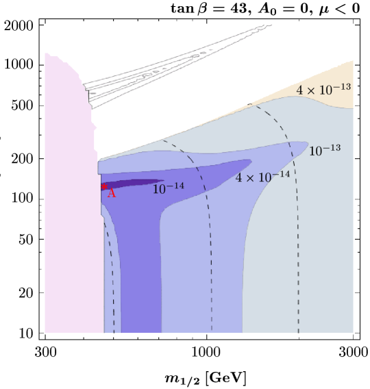
Figure 5.7 shows contours of constant in the (, ) plane for , , and a negative sign of the parameter. The contour lines represent the values , , , and , where darker shadings imply smaller values of . The dashed lines are contours of , and (from left to right). The light-shaded region at is excluded by the mass bound from Higgs searches at LEP [32]. The white area indicates the region in which either correct electroweak symmetry breaking is not established (in the very upper left corner) or in which . Since , the plane is actually in tension because of (negative) SUSY contributions to the anomalous magnetic moment of the muon, .
Figure 5.8 presents a scan over the (, ) plane for , , and
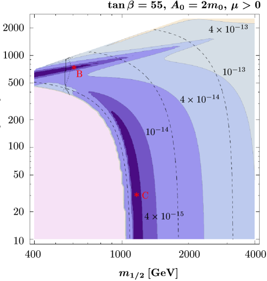
with contours of , , , , and (darker shadings indicate smaller values) and , , and (dashed lines, from left to right). The large light-shaded region in the lower left corner is excluded by the robust bound [32] from collider searches of charged sleptons (or by the appearance of a tachyonic spectrum). The LEP Higgs bound [32] is situated within this region in close vicinity to its boundary for and is indicated by the solid line for . In the region to the left of the dotted line, [212], which is in tension with the bounds from inclusive decays.
Let us now discuss some generic features of the stau yield within the CMSSM on the basis of Figs. 5.7 and 5.8. We note beforehand that our more general statements on the NLSP region in the CMSSM are corroborated by a parameter scan over the following range131313Here, we disregard CMSSM parameter points in which SPheno flags an error in the spectrum calculation.
| (5.23) |
In both figures an almost horizontal, narrow band of low appears in which holds so that stau annihilation proceeds via resonant production of the heavy CP-even Higgs boson . We have marked points the centers of the respective regions with “A” and “B” for which we provide detailed information in Table 5.2. Given a present uncertainty of in the determination of [213], we note that the LEP Higgs bound has to be treated with some care. For example, a (vertical) contour would be situated at in the resonance region of Fig. 5.8. Accordingly, one could consider the entire resonance region shown to be compatible with direct Higgs searches. However, due to the large value of , the bound on is very strong so that a large part of the resonance region remains excluded by this constraint. In this regard, it is interesting to see (Fig. 5.7) that also appears in the NLSP region for lower values of . In the center of both resonance regions, the yield becomes as low as (point A) and (point B). Despite the heavier mass of the lighter stau (see Table 5.2), the suppression of is still more pronounced in Fig. 5.8 than in Fig. 5.7. This is because the bottom Yukawa coupling becomes larger with increasing , as discussed already in Sec. 5.5. In fact, annihilation into final states is in both cases by far the dominant process with relative importance of (point A) and (point B). The extension of both resonance regions is due to the total width of of respectively (point A) and (point B); note the logarithmic scales in Figs 5.7 and 5.8. We note in passing that the appearance of the resonance does not imply the absence of the neutralino funnel region which is indicated by the (unshaded) contour lines in the white area of Fig. 5.7
Of course, the question arises whether the appearance of the resonance region is encountered more generically within the framework of the CMSSM. In principle, it is not easy to provide a simple quantitative connection between and for arbitrary values of the CMSSM parameters. However, without emphasis on an overall applicability, a qualitative picture can be drawn. Let us start with the mass of the CP-odd Higgs boson which can be written as [214, 215]
| (5.24) |
Here, the ellipsis stand for contributions from the bottom and tau Yukawa couplings. For , , and the corrections from the bottom and tau Yukawa couplings become important so that is driven towards lower values;141414The latter relation ignores contributions from -terms which can be important but complicate the envisaged illustrative picture; for the derivation, we have used in Eq. (2.25a) of Ref. [215]. note that for . Indeed, this property can be used to constrain from above by confronting with the lower bound from LEP, [32]. On the other hand, for large , one also enters the decoupling limit of the MSSM so that and will be nearly degenerate in mass; cf. (5.13). This can be also seen from the exemplary points presented in Table 5.2. Therefore, also will be driven towards lower values for growing . Now, left-right mixing of the lighter stau for not too large values of is small within the CMSSM, , so that approximately [215]. Therefore, is the relation that holds usually in the region in which is the lightest Standard Model superpartner. However, for large , the contributions from the bottom Yukawa coupling in (5.24) can become strong enough (growing with [215]) to overcome any additional decrease of due to left-right mixing so that the resonance condition can indeed be met. Nevertheless, from scanning over the CMSSM parameter range (5.7) it seems to us that the resonance condition is not easily realized in the part of the NLSP region in which - coannihilations are negligible. Conversely, it is clear that relaxing the universality conditions for the soft-SUSY breaking masses at will make it easier to find parameter regions in which the resonance condition is satisfied. Of particular interest in this respect is the model with non-universal Higgs masses (NUHM) with at . There, one can adjust the input parameters in order to realize resonant stau annihilation. Indeed, this model is qualitatively the same as the class of pMSSM scenarios considered in the previous sections, where and are traded (at the low-scale) against and by using the electroweak symmetry breaking conditions.
Low values are also realized in the narrow vertical region around in Fig. 5.8. At the representative point “C” of that region, and the main stau annihilation channels are the ones into () and (); see Table 5.2. For larger values of , exhibits its well known behavior and grows with . To the left of the contour, the yield increases quickly since the annihilation into becomes kinematically forbidden. Indeed, regions of low which are due to the aforementioned annihilation channels are a commonplace appearance in the CMSSM parameter space. They are found slightly above the lowest feasible values of , i.e., close to the boundary of the region which is excluded by direct Higgs and SUSY searches and where still holds. This is because is light in that region since the SUSY particle spectrum scales with (typically, for NLSP). Moreover, we find that the LEP Higgs bound drops hardly below for and .151515The position of the LEP Higgs bound (which appears as a near to vertical line for low ) is very sensitive to the value of . Lowering shifts the bound towards larger values of . Due to a strong correlation between the gaugino mass parameter and the size of the parameter, [216], the value of in the experimentally allowed region is large. Recall from Sec. 5.4 that the coupling is () so that will become sizeable by increasing . This leads then to efficient stau annihilation into final states. Indeed, in those CMSSM regions, also is maximized so that already starts to drop below the estimate (4.1) for . Note, however, that the left-right mixing of within the CMSSM is somewhat constrained. Neglecting -Yukawa contributions, the RG-evolution induced splitting reads [215] and indeed remains mainly right-handed: By scanning over the parameter space, we typically find and thus in the NLSP region in which and holds.
| Point | A | B | C | |
|---|---|---|---|---|
| 456 | 600 | 1138 | ||
| 124 | 748 | 30 | ||
| 43 | 55 | 55 | ||
| 130 | 197 | 127 | ||
| 352 | 673 | 739 | ||
| 114 | 80 | 75 | ||
| 114.6 | 115 | 117.9 | ||
| 265 | 390 | 799 | ||
| 9.6 | 22 | 41 | ||
| -565 | 666 | 1262 | ||
| -63 | 473 | -164 | ||
| 1052 | 1375 | 2446 | ||
| 740 | 1091 | 1757 | ||
| 76 | 87 | |||
| 10 | 90 | |||
| 9 | 11 | |||
| 2 | 6 | |||
| 30 | 30 | 32 | ||
| 4.2 | 2.5 | 2.2 | ||
| 100 | 100 | 100 | ||
| (50) | (50) | (50) | ||
| () | () | () | ||
| () | () | () |
5.8 Prospects for collider phenomenology
If a SUSY model with a long-lived of is realized in nature, the discovery potential will be promising at the LHC with a luminosity of 100 fb-1 [141]. For (0.5 TeV), ’s can also be examined in precision studies at the ILC with a c.m. range up to (1 ). Once long-lived ’s are produced, one should be able to distinguish them from muons by considering the associated highly ionizing tracks and with time-of-flight measurements. One should then also be able to infer from measurements of the velocity and its momentum [217] and complementary from (threshold) studies of the process at the ILC.
Both mechanisms leading to exceptionally small values come with testable predictions: certain ranges of the stau-mixing angle together with large values of , , and/or and, in the case of resonant stau annihilation, also . In particular, the large stau-Higgs couplings lead to an enhanced production of light Higgs bosons in association with staus via and . The associated cross sections can then be relatively large at the ILC with a sufficiently high c.m. energy [218]. In addition, the above reactions with instead of in the final state can have also relatively large cross sections if and are sufficiently light. These reactions will then allow for an experimental determination of the stau-Higgs couplings and clarify whether its values are compatible with an extremely small value of [218]. Moreover, a measurement of pointing to could be an experimental hint for resonant stau annihilation in the early Universe.
Indeed, the scenarios considered could allow for a determination of both and already at the LHC. Because of the large values of , the dominant production mechanism for will be the associated production of the neutral Higgs bosons with bottom quark pairs, ; see, e.g., [219, 220, 221] and references therein. In fact, associated production with is considered as one of the most promising processes for measurements of at the LHC despite the relatively small branching ratio [222]. In SUSY scenarios with a sufficiently light long-lived NLSP, these processes will be complemented by associated production with , where measurements of the invariant mass of the pair could potentially provide a unique way to infer and at the LHC. In fact, will occur most prominently exactly in the regions associated with the exceptional values due to the enhanced stau–Higgs couplings. Having outlined these proposals, we leave a dedicated study for future work.
Table 5.2 illustrates that the kinematical reach of both the LHC and the ILC could be sufficiently large to allow for the studies mentioned above. In none of the given points does exceed so that pair production would already be possible at the ILC with . There, one could also produce final states in scenarios A and C. Even the condition could be probed in both scenarios A and B that allow for resonant stau annihilation.
5.9 Implications for gravitino dark matter scenarios
We have seen in this thesis that is subject to stringent cosmological constraints. Indeed, to decide on the cosmological viability of a SUSY model, one has to confront the associated values with those constraints. For gravitino LSP scenarios with unbroken R-parity, we have obtained restrictive cosmological constraints in Part II. In particular, in Sects. 4.1, 4.2.1, and 4.2.2 we have derived constraints and implications thereof under the assumption that can be described by (4.3). However, while (4.3) is quite reliable for [31, 138, 1, 36], we have shown in the previous sections that (for a given ) can be about two orders of magnitude smaller than (4.3).
Generally speaking, in this chapter we have shown that islands exist in which can be significantly below (4.3) even within the CMSSM and for a standard cosmological history. Thus, in gravitino dark matter scenarios with such exceptionally small values, our understanding of the cosmological constraints and the associated implications could change significantly. To demonstrate this point, let us indicate for which values the existing cosmological constraints are respected:
-
•
For , the upper limit on imposed by the non-thermal production of gravitinos in decays, —given explicitly in (22) of Ref. [139]—is respected for even if only a small fraction of dark matter is assumed to originate from decays; cf. Fig. 13 of Ref. [139]. This applies equally to other scenarios with an extremely weakly interacting LSP—such as the axino LSP [223, 188, 224]—originating from decays.
-
•
For , the BBN constraints associated with effects of hadronic energy release on the primordial D abundance can be respected for and up to independent of the lifetime; cf. Fig. 11 of Ref. [139]. For a sizable admixture of in , this constraint can become more restrictive in particular with the enhanced stau–Higgs couplings allowing for exceptionally small values. Nevertheless, these exceptional values are typically associated with where the limit is significantly more relaxed: for . A tightening to () will then require an increase of (hadronic) by a factor of (). On the other hand, sufficiently degenerate and will always be associated with small values of and thereby with relaxed limits from energy release, even in the case of strongly enhanced stau–Higgs couplings.
- •
-
•
For , the BBN constraints associated with bound state effects allowing for CBBN of 6Li and 9Be can be respected even for ; see Fig. 2.9. Recall, that these values correspond to upper limits on the primordial fractions of 9Be/H and 6Li/H of and to the generous range , respectively.
Thus, the SUSY models which come with thermal relic stau abundances of can respect each of those cosmological constraints independently of the stau lifetime if a primordial 6Li/H abundance of about is viable. In particular, the limit (4.8) of and its implications discussed in Chapter 4 are then no longer valid even for a standard cosmological history with primordial temperatures of . Thereby, the regions with are associated with particularly attractive gravitino dark matter scenarios:
-
•
The gravitino mass can be within the range for which its kinematical determination could be viable [154, 190, 191]. Together with measurements of and , a kinematically determined would allow one to measure the Planck scale at colliders [154, 190, 191]. Indeed, an agreement of the value determined in collider experiments with the one inferred from Newton’s constant would support the existence of supergravity in nature [154].
-
•
For sufficiently close to , the spin-3/2 character of the gravitino becomes relevant so that it could be probed in principle by analyzing the decays [154].
-
•
With , is negligible so that basically all of can be provided by gravitinos from other sources such as thermal production. Indeed, if also gravitino production in decays of scalar fields such as the inflaton [121, 123] is negligible, reheating temperatures of could become viable for and not too heavy gaugino masses; see, in particular, Sec. 3.4. This would mean that thermally produced gravitinos could provide the right amount of dark matter and that thermal leptogenesis (with as a benchmark value [134, 135]) would be a viable explanation of the cosmic baryon asymmetry, i.e., there would be no gravitino problem.
-
•
With a kinematically determined , one would be able to probe the reheating temperature at colliders and thereby the viability of thermal leptogenesis [119].
-
•
For , the small values could still allow for the primordial catalysis of 6Li and 9Be in agreement with existing astrophysical observations; see Sec. 2.6.
Table 5.2 illustrates that gravitino dark matter scenarios of the type discussed above can even be accommodated within the CMSSM. For gravitino masses of and , we list the associated values of , of , and of the maximum reheating temperature under the assumption that other gravitino sources can be neglected. The stau lifetime is given in (4.4) and the values imposed by can be inferred from (4.12). At each CMSSM point and for both values, is very long lived, , and gravitino production from decays is negligible, . In all cases, the gravitino mass is sufficiently close to so that the spin-3/2 character of the gravitino can in principle be probed [154]. A reheating temperature of is viable only for the points A and B with significantly below , i.e., at the points at which resonant stau annihilation leads to the reduction of . Because of , the limit from CBBN of 9Be is at for each point as can be inferred from Fig. 2.9. This bound disfavors point A while the points B and C are associated with values very close to this limit and thereby with () values of about ().
Conclusions
In this thesis we have worked out the cosmological implications of a long-lived electromagnetically charged massive particle species also called CHAMP. Our working hypothesis has been that possesses a weak-scale mass and typically a lifetime . We have assumed that the temperature of the early Universe was high enough so that has achieved chemical equilibrium with the primordial plasma. Then, following a standard cosmological evolution, experienced a thermal freeze-out once . This makes to what is called a thermal relic (prior to its decay).
BBN with a long-lived CHAMP
We have started our investigation with a brief introduction into the framework of standard Big Bang Nucleosynthesis (SBBN) where we also have given account to some of the latest measurements from which primordial light element abundances are inferred. In a simplified discussion of -decoupling we have argued that its expected cosmological abundance prior to decay reads . We have recalled that the long-lived CHAMP scenario is strongly constrained by BBN limits on electromagnetic and hadronic energy release in the -decay. For a reliability check on hadronic BBN constraints we have worked out the Coulomb stopping power of charged hadrons in the plasma. In particular, we have developed on a refined approach taking into account peculiarities in the plasma-screening of the Coulomb interaction and paying close attention to the velocity dependencies of the cross sections. We find reasonably good agreement with the treatment used in Ref. [41] from which we have incorporated the associated constraints.
Subsequently, the effects of on BBN due to its binding onto the light nuclei have been considered. Given that the -catalysis of thermal nucleosynthesis reactions had only been discovered recently [79], we have laid out in detail the central points of CBBN. Using the variational approach, we have obtained ground state energies for bound states by taking into account the finite nuclear charge radius of . This leads to a reduction (in magnitude) from the naïve point-like Coulomb values, e.g., for by and for by which has also been confirmed upon numerical solution of the Schrödinger equation. For the examples of and also the complete spectrum for has been computed. We have further obtained the wave functions for the –continuum. This has allowed us to calculate the cross sections for photo-dissociation, , and radiative recombination, , including the finite charge radius correction and taking into account recombinations into 1S as well as 2S states. Those rates (per particle pair) are important since they control the fractional bound state abundance and thus the timing and efficiency of CBBN. For example, for and we find a reduction of from the hydrogen-like case by and by , respectively.
From observations of beryllium in Population II halo stars at very low metallicities, we have extracted a nominal upper limit on primordial beryllium of . This limit allows one to set constraints on models in which the primordial divide is bridged by catalytic effects. Considering the primordial catalysis of 9Be [63], we have derived -dependent upper limits on the -yield prior to decay, . For a typical relic abundance (), we find that this limit translates into an upper limit on the lifetime of (). Furthermore, we have also worked out the catalytic production of which, depending on the adopted upper limit on primordial , gives rise to similar bounds.
We have clarified that the presence of () bound states cannot relax the limits at long lifetimes in any substantial way. Indeed, we have shown explicitly by solving the associated full set of Boltzmann equations that late-time effects of () bound states can affect the lithium and beryllium abundances synthesized at by not more than a few percent. Any substantial formation of () at is immediately intercepted by the very efficient charge exchange reaction of () with . This comes as no surprise given the large size of the () system and the fact that the proton deconfinement probability approaches unity already for a – distance of . In particular, we find that the fractional density of protons in bound states does not exceed the level of for . By the same argument, the yield also remains unaffected by late-time catalysis. Thus, we find that the possibility of allowed islands in the parameter region with typical and large —which was advocated in Ref. [90]—does not exist.
The gravitino-stau scenario
In the second part of this thesis we have considered cosmological constraints and their implications for models in which the gravitino is the LSP and the stau is the NLSP. We have first focused on as a dark matter candidate. Using the full gauge-invariant result for the thermally produced gravitino abundance to leading order in the Standard Model gauge couplings [108, 119], we have studied bounds on the reheating temperature from the constraint . In particular, taking into account the dependence of on the masses of the gauginos has allowed us to explore the dependence of the bounds on the gaugino-mass relation at the scale of grand unification . We have explicitly studied the effect of regeneration during a post-inflationary perturbative reheating phase. Thereby, we have made contact between the notion of as the initial temperature of the radiation-dominated epoch in the analytical expression (3.6) for the abundance and the definition of in terms of the decay width of the inflaton.
Applying the -dependent upper limits on derived from the primordial catalysis of and in Part I, we have analyzed the emerging constraints in the gravitino-stau scenario, i.e., for . For typical values (4.3) of the stau NLSP yield after decoupling, the and constraints have been found in close vicinity to each other so that they lead to the same implications. For example, for , the CBBN constraints impose the lower limit with rising tendency for growing . For being the lightest Standard Model superpartner such a limit directly affects the testability of those SUSY scenarios at future colliders. Furthermore, for a primordial limit of the calculated abundance drops below this observational bound only for (likewise for ). Taken at face value, we find that this constraint translates into a lower limit on the gaugino mass parameter in the entire natural region of the CMSSM parameter space. This limit implies a restrictive upper bound .
Using exemplary (,) CMSSM planes where we explicitly compute in every point, we have further explored gravitino dark matter scenarios and the associated bounds for and for temperatures as low as . Taking into account the CBBN constraint as well as the constraints on electromagnetic and hadronic energy injection from -decays, we have illustrated that in the considered regions of the CMSSM parameter space indeed is the highest cosmologically viable temperature of the radiation-dominated epoch in case of a standard thermal history of the Universe. Moreover, in the NLSP region the lower bound on typically implies a very heavy superparticle mass spectrum where, e.g., can be well excluded and which makes such scenarios hard to probe at the LHC. The bound on imposes a serious constraint for inflation models. Moreover, thermal leptogenesis seems to be strongly disfavored in the considered regions of the CMSSM parameter space.
With late-time entropy release, the obtained limit can be relaxed. For example, the dilution of the thermally produced gravitino yield by a factor of relaxes the bound by about one order of magnitude in regions where dominates . In the case of entropy production after NLSP decoupling, the yield of the NLSP prior to its decay, , is reduced so that the BBN constraints can be weakened. Although the 6Li bound is persistent, we find that it disappears provided is diluted by a factor of . We have discussed the viability of thermal leptogenesis in a cosmological scenario with entropy production after NLSP decoupling. We find that successful thermal leptogenesis can be revived in generic regions of the CMSSM parameters space for and , where is the mass of the lightest among the heavy right-handed Majorana neutrinos. There, the collider-friendly NLSP region with reopens as a cosmologically allowed region in the CMSSM with the gravitino LSP.
Thermal relic stau abundances
In the final part of this thesis we have carried out a thorough study of primordial stau annihilation and the associated thermal freeze-out. Taking into account the complete set of stau annihilation channels within the MSSM with real parameters for cases with negligible sparticle coannihilation, the resulting thermal relic yield has been examined systematically. While we have often (implicitly) focused on the case in Part II by employing (4.3), we have investigated cases in Part III in which contains a significant admixture of including the maximal mixing case as well as .
We find that the variation of the stau mixing angle affects the relative importance of the different annihilation channels significantly but not necessarily the resulting value for relatively small values of . By increasing , however, we encounter a dramatic change of this picture for large absolute values of the Higgs-higgsino mass parameter and/or of the trilinear coupling , which are the dimensionful SUSY parameters that govern simultaneously stau left-right mixing and the stau–Higgs couplings: Stau annihilation into , , and can become very efficient (if kinematically allowed) so that can decrease to values well below . The scalar nature of allows those parameters to enter directly into the annihilation cross sections. This mechanism has no analogue in calculations of the thermal relic density of the lightest neutralino .
The stau–Higgs couplings are crucial also for the second reduction mechanism identified in this work: Even for moderate values of , we find that staus can annihilate very efficiently into a pair via -channel exchange of the heavy CP-even Higgs boson provided the MSSM spectrum exhibits the resonance condition . We have shown explicitly that the associated values can be below as well. This mechanism is similar to the one that leads to the reduction of the density in the Higgs funnel region in which neutralino annihilation proceeds at the resonance of the CP-odd Higgs boson .
We have worked with an effective low energy version of the MSSM to investigate the -dependence of and the two -reduction mechanisms in a controlled way. In addition, we have shown that the considered effects can be accommodated also with restrictive assumptions on the soft-SUSY breaking sector at a high scale. Within the CMSSM, we encounter both mechanisms each of which leading to in two distinct regions of a single plane.
We have discussed possibilities to probe the viability of the presented -reduction mechanisms at colliders. While a measurement pointing to would support resonant primordial stau annihilation, studies of Higgs boson production in association with staus, could allow for an experimental determination of the relevant stau–Higgs couplings, for example, at the ILC. Moreover, we have outlined that associated production with has the potential to allow for a determination of both and at the LHC if a SUSY scenario with large and large stau–Higgs couplings is realized.
With the obtained small values, even the restrictive constraints associated with CBBN could be respected so that attractive gravitino dark matter scenarios could be revived to be cosmologically viable even for a standard cosmological history. Within this class of models, collider evidence for supergravity, for the gravitino being the LSP, and for high values of the reheating temperatures of up to is conceivable, which could thereby accommodate simultaneously the explanation of the cosmic baryon asymmetry provided by thermal leptogenesis and the hypothesis of thermally produced gravitinos being the dark matter in our Universe.
References
- [1] J. Pradler and F. D. Steffen, Constraints on the reheating temperature in gravitino dark matter scenarios, Phys. Lett. B648 (2007) 224–235 [hep-ph/0612291].
- [2] J. Pradler and F. D. Steffen, Implications of Catalyzed BBN in the CMSSM with Gravitino Dark Matter, Phys. Lett. B666 (2008) 181–184 [0710.2213].
- [3] J. Pradler and F. D. Steffen, CBBN in the CMSSM, Eur. Phys. J. C56 (2008) 287–291 [0710.4548].
- [4] M. Pospelov, J. Pradler and F. D. Steffen, Constraints on Supersymmetric Models from Catalytic Primordial Nucleosynthesis of Beryllium, JCAP 0811 (2008) 020 [0807.4287].
- [5] J. Pradler and F. D. Steffen, Thermal relic abundances of long-lived staus, Nucl. Phys. B809 (2009) 318–346 [0808.2462].
- [6] WMAP Collaboration, D. N. Spergel et. al., First Year Wilkinson Microwave Anisotropy Probe (WMAP) Observations: Determination of Cosmological Parameters, Astrophys. J. Suppl. 148 (2003) 175–194 [astro-ph/0302209].
- [7] D. N. Spergel et. al., Wilkinson microwave anisotropy probe (WMAP) three year results: Implications for cosmology, Astrophys. J. Suppl. 170 (2007) 377 [astro-ph/0603449].
- [8] E. Komatsu et. al., Five-Year Wilkinson Microwave Anisotropy Probe (WMAP) Observations: Cosmological Interpretation, Astrophys. J. Suppl. 180 (2009) 330–376 [0803.0547].
- [9] J. Dunkley et. al., Five-Year Wilkinson Microwave Anisotropy Probe (WMAP) Observations: Likelihoods and Parameters from the WMAP data, Astrophys. J. Suppl. 180 (2009) 306–329 [0803.0586].
- [10] G. Steigman, The cosmological evolution of the average mass per baryon, JCAP 0610 (2006) 016 [astro-ph/0606206].
- [11] M. Pettini, B. J. Zych, M. T. Murphy, A. Lewis and C. C. Steidel, Deuterium Abundance in the Most Metal-Poor Damped Lyman alpha System: Converging on , 0805.0594.
- [12] V. Simha and G. Steigman, Constraining The Universal Lepton Asymmetry, JCAP 0808 (2008) 011 [0806.0179].
- [13] G. Steigman, Primordial Nucleosynthesis in the Precision Cosmology Era, Ann. Rev. Nucl. Part. Sci. 57 (2007) 463–491 [0712.1100].
- [14] R. H. Cyburt, B. D. Fields and K. A. Olive, An update on the big bang nucleosynthesis prediction for Li-7: The problem worsens, JCAP 0811 (2008) 012.
- [15] F. Spite and M. Spite, Abundance of lithium in unevolved halo stars and old disk stars: Interpretation and consequences, Astron. Astrophys. 115 (1982) 357–366.
- [16] M. Asplund, N. Grevesse and A. J. Sauval, The Solar Chemical Composition, vol. 336 of Astronomical Society of the Pacific Conference Series. Barnes, III, T. G. and Bash, F. N., Sept., 2005.
- [17] S. G. Ryan, J. E. Norris and T. C. Beers, The Spite Lithium Plateau: Ultra-Thin but Post- Primordial, Astrophys. J. 523 (1999) 654–677 [astro-ph/9903059].
- [18] M. Asplund, D. L. Lambert, P. E. Nissen, F. Primas and V. V. Smith, Lithium isotopic abundances in metal-poor halo stars, Astrophys. J. 644 (2006) 229–259 [astro-ph/0510636].
- [19] P. Bonifacio, P. Molaro, T. Sivarani, R. Cayrel, M. Spite, F. Spite, B. Plez, J. Andersen, B. Barbuy, T. C. Beers, E. Depagne, V. Hill, P. François, B. Nordström and F. Primas, First stars VII - Lithium in extremely metal poor dwarfs, A&A 462 (Feb., 2007) 851–864 [astro-ph/0610245].
- [20] W. Aoki et. al., Lithium Abundances of Extremely Metal-Poor Turn-off Stars, Astrophys. J. 698 (2009) 1803–1812 [0904.1448].
- [21] V. V. Smith, D. L. Lambert and P. E. Nissen, The 6Li/7Li ratio in the metal-poor halo dwarfs HD 19445 and HD 84937, ApJ 408 (May, 1993) 262–276.
- [22] L. M. Hobbs and J. A. Thorburn, Lithium isotope ratios in six halo stars, ApJ 428 (June, 1994) L25–L28.
- [23] V. V. Smith, D. L. Lambert and P. E. Nissen, Isotopic Lithium Abundances in Nine Halo Stars, ApJ 506 (Oct., 1998) 405–423.
- [24] R. Cayrel, M. Spite, F. Spite, E. Vangioni-Flam, M. Cassé and J. Audouze, New high S/N observations of the 6Li/7Li blend in HD 84937 and two other metal-poor stars, A&A 343 (Mar., 1999) 923–932 [astro-ph/9901205].
- [25] C. P. Deliyannis, P. Demarque and S. D. Kawaler, Lithium in halo stars from standard stellar evolution, ApJS 73 (May, 1990) 21–65.
- [26] M. H. Pinsonneault, C. P. Deliyannis and P. Demarque, Evolutionary models of halo stars with rotation. II - Effects of metallicity on lithium depletion, and possible implications for the primordial lithium abundance, ApJS 78 (Jan., 1992) 179–203.
- [27] F. Takayama, Extremely Long-Lived Charged Massive Particles as a Probe for Reheating of the Universe, Phys. Rev. D77 (2007) 116003 [0704.2785].
- [28] P. Gondolo and G. Gelmini, Cosmic abundances of stable particles: Improved analysis, Nucl. Phys. B360 (1991) 145–179.
- [29] K. Griest and D. Seckel, Three exceptions in the calculation of relic abundances, Phys. Rev. D43 (1991) 3191–3203.
- [30] M. Drees, R. Godbole and P. Roy, Theory and phenomenology of Sparticles: An account of four- dimensional supersymmetry in high energy physics, . Hackensack, USA: World Scientific (2004) 555 p.
- [31] T. Asaka, K. Hamaguchi and K. Suzuki, Cosmological gravitino problem in gauge mediated supersymmetry breaking models, Phys. Lett. B490 (2000) 136–146 [hep-ph/0005136].
- [32] Particle Data Group Collaboration, W. M. Yao et. al., Review of particle physics, J. Phys. G33 (2006) 1–1232.
- [33] P. Gondolo et. al., DarkSUSY: Computing supersymmetric dark matter properties numerically, JCAP 0407 (2004) 008 [astro-ph/0406204].
- [34] J. M. Blatt and V. F. Weisskopf, Theoretical nuclear physics. John Wiley & Sons Inc., New York, 1952.
- [35] T. K. Hemmick et. al., A search for anomalously heavy isotopes of low nuclei, Phys. Rev. D41 (1990) 2074–2080.
- [36] C. F. Berger, L. Covi, S. Kraml and F. Palorini, The number density of a charged relic, JCAP 0810 (2008) 005 [0807.0211].
- [37] M. H. Reno and D. Seckel, Primordial Nucleosynthesis: The Effects of Injecting Hadrons, Phys. Rev. D37 (1988) 3441.
- [38] S. Dimopoulos, R. Esmailzadeh, L. J. Hall and G. D. Starkman, Limits on late decaying particles from nucleosynthesis, Nucl. Phys. B311 (1989) 699.
- [39] R. H. Cyburt, J. R. Ellis, B. D. Fields and K. A. Olive, Updated nucleosynthesis constraints on unstable relic particles, Phys. Rev. D67 (2003) 103521 [astro-ph/0211258].
- [40] K. Jedamzik, Did something decay, evaporate, or annihilate during big bang nucleosynthesis?, Phys. Rev. D70 (2004) 063524 [astro-ph/0402344].
- [41] M. Kawasaki, K. Kohri and T. Moroi, Big-bang nucleosynthesis and hadronic decay of long-lived massive particles, Phys. Rev. D71 (2005) 083502 [astro-ph/0408426].
- [42] S. Bailly, K. Jedamzik and G. Moultaka, Gravitino Dark Matter and the Cosmic Lithium Abundances, 0812.0788.
- [43] M. Kawasaki and T. Moroi, Electromagnetic cascade in the early Universe and its application to the big bang nucleosynthesis, Astrophys. J. 452 (1995) 506 [astro-ph/9412055].
- [44] G. Audi, A. H. Wapstra and C. Thibault, The Ame2003 atomic mass evaluation (II). Tables, graphs and references, Nucl. Phys. A729 (2002) 337–676.
- [45] K. Jedamzik, Lithium-6: A Probe of the Early Universe, Phys. Rev. Lett. 84 (2000) 3248 [astro-ph/9909445].
- [46] K. Jedamzik, Neutralinos and Big Bang nucleosynthesis, Phys. Rev. D70 (2004) 083510 [astro-ph/0405583].
- [47] M. Kawasaki, K. Kohri and T. Moroi, Hadronic decay of late-decaying particles and big-bang nucleosynthesis, Phys. Lett. B625 (2005) 7–12 [astro-ph/0402490].
- [48] V. B. Berestetsky, E. M. Lifshitz and L. P. Pitaevsky, Quantum Electrodynamics. Oxford, Uk: Pergamon 652 P. ( Course Of Theoretical Physics, 4), 1982.
- [49] R. G. Sachs, High-Energy Behavior of Nucleon Electromagnetic Form Factors, Phys. Rev. 126 (1962) 2256–2260.
- [50] M. N. Rosenbluth, High Energy Elastic Scattering of Electrons on Protons, Phys. Rev. 79 (1950) 615–619.
- [51] R. C. Walker et. al., Measurements of the proton elastic form-factors for at SLAC, Phys. Rev. D49 (1994) 5671–5689.
- [52] R. Schiavilla and I. Sick, Neutron charge form factor at large , Phys. Rev. C64 (2001) 041002 [nucl-ex/0107004].
- [53] G. G. Raffelt, Astrophysical axion bounds diminished by screening effects, Phys. Rev. D33 (1986) 897.
- [54] G. G. Raffelt, Stars as laboratories for fundamental physics: The astrophysics of neutrinos, axions, and other weakly interacting particles. Chicago, USA: Univ. Pr. 664 p, 1996.
- [55] T. Hahn, Cuba: A library for multidimensional numerical integration, Comput. Phys. Commun. 168 (2005) 78–95 [hep-ph/0404043].
- [56] J. Bernstein, Kinetic theory in the expanding universe. Cambridge, USA: Univ. Pr. 149p, 1988.
- [57] T. Bringmann and S. Hofmann, Thermal decoupling of WIMPs from first principles, JCAP 0407 (2007) 016 [hep-ph/0612238].
- [58] E. M. Lifshitz, L. D. Landau and L. P. Pitaevskii, Electrodynamics of continuous media. Pergamon Press, 1984.
- [59] J. D. Jackson, Classical electrodynamics. John Wiley & Sons Inc., New York, 1975.
- [60] E. Braaten and M. H. Thoma, Energy loss of a heavy fermion in a hot plasma, Phys. Rev. D44 (1991) 1298–1310.
- [61] I. Angeli, A consistent set of nuclear rms charge radii: properties of the radius surface R(N,Z), Atomic Data and Nuclear Data Tables 87 (July, 2004) 185–206.
- [62] L. Visscher and K. G. Dyall, Dirac-Fock Atomic Electronic Structure Calculations Using Different Nuclear Charge Distributions, Atomic Data and Nuclear Data Tables 67 (1997) 207.
- [63] M. Pospelov, Bridging the primordial A=8 divide with Catalyzed Big Bang Nucleosynthesis, 0712.0647.
- [64] M. Kamimura, Y. Kino and E. Hiyama, Big-Bang Nucleosynthesis Reactions Catalyzed by a Long- Lived Negatively-Charged Leptonic Particle, 0809.4772.
- [65] E. Hiyama, M. Kamimura, T. Motoba, T. Yamada and Y. Yamamoto, Three- and four-body cluster models of hypernuclei using the G-matrix N interaction: , , and , Prog. Theor. Phys. 97 (1997) 881–899.
- [66] F. L. Yost, J. A. Wheeler and G. Breit, Coulomb Wave Functions in Repulsive Fields, Phys. Rev. 49 (1936) 174–189.
- [67] M. L. Goldberger and K. M. Watson, Collision theory. New York : Wiley, c1964. Structure of matter series, 1964.
- [68] M. Abramowitz and I. A. Stegun, Handbook of Mathematical Functions with Formulas, Graphs, and Mathematical Tables. Dover, New York, tenth ed., 1964.
- [69] E. T. Whittaker and G. N. Watson, A course of modern analysis. Cambridge: University Press, 4th ed., 1963.
- [70] A. Burgess and M. J. Seaton, A general formula for the calculation of atomic photo-ionization cross-sections, MNRAS 120 (1960) 121.
- [71] M. J. Seaton, The Quantum Defect Method, MNRAS 118 (1958) 504.
- [72] J. G. Beckerley, Expansion of positive energy Coulomb wave functions in powers of the energy, Phys. Rev. 67 (Jan, 1945) 11–14.
- [73] K. Kohri and F. Takayama, Big Bang Nucleosynthesis with Long Lived Charged Massive Particles, Phys. Rev. D76 (2007) 063507 [hep-ph/0605243].
- [74] L. D. Landau and E. M. Lifshitz, Quantum mechanics. Course of theoretical physics, Oxford: Pergamon Press, 1965, 1965.
- [75] C. Bird, K. Koopmans and M. Pospelov, Primordial Lithium Abundance in Catalyzed Big Bang Nucleosynthesis, Phys. Rev. D78 (2008) 083010 [hep-ph/0703096].
- [76] S. Dimopoulos, D. Eichler, R. Esmailzadeh and G. D. Starkman, Getting a charge out of dark matter, Phys. Rev. D41 (1990) 2388.
- [77] A. De Rujula, S. L. Glashow and U. Sarid, Charged Dark Matter, Nucl. Phys. B333 (1990) 173.
- [78] J. Rafelski, M. Sawicki, M. Gajda and D. Harley, Reactions of charged massive particle in a deuterium environment, Phys. Rev. A44 (1991) 4345.
- [79] M. Pospelov, Particle physics catalysis of thermal big bang nucleosynthesis, Phys. Rev. Lett. 98 (2007) 231301 [hep-ph/0605215].
- [80] C. Angulo et. al., A compilation of charged-particle induced thermonuclear reaction rates, Nucl. Phys. A656 (1999) 3–183.
- [81] R. H. Cyburt and B. Davids, Evaluation of Modern Be Data, Phys. Rev. C78 (2008) 064614 [0809.3240].
- [82] K. M. Nollett, R. B. Wiringa and R. Schiavilla, A six-body calculation of the alpha-deuteron radiative capture cross section, Phys. Rev. C63 (2001) 024003 [nucl-th/0006064].
- [83] O. Pisanti et. al., PArthENoPE: Public Algorithm Evaluating the Nucleosynthesis of Primordial Elements, Comp. Phys. Commun. 178 (2008) 956 [0705.0290].
- [84] K. Hamaguchi, T. Hatsuda, M. Kamimura, Y. Kino and T. T. Yanagida, Stau-catalyzed Li-6 production in big-bang nucleosynthesis, Phys. Lett. B650 (2007) 268–274 [hep-ph/0702274].
- [85] P. J. Mohr and B. N. Taylor, CODATA recommended values of the fundamental physical constants: 2002, Rev. Mod. Phys. 77 (2005) 1–107.
- [86] G. R. Caughlan and W. A. Fowler, Thermonuclear reaction rates. 5, Atom. Data Nucl. Data Tabl. 40 (1988) 283–334.
- [87] D. Thomas, D. N. Schramm, K. A. Olive and B. D. Fields, Primordial nucleosynthesis and the abundance of beryllium and boron, Astrophys. J. 406 (1993) 569–579 [astro-ph/9206002].
- [88] V. F. Mukhanov, Nucleosynthesis Without a Computer, Int. J. Theor. Phys. 43 (2004) 669–693 [astro-ph/0303073].
- [89] L. Kawano, Let’s go: Early Universe. 2. Primordial nucleosynthesis: The Computer way, . FERMILAB-PUB-92-004-A.
- [90] K. Jedamzik, The cosmic 6Li and 7Li problems and BBN with long-lived charged massive particles, Phys. Rev. D77 (2008) 063524 [0707.2070].
- [91] R. Svensson and A. Zdziarski, Photon-photon scattering of gamma rays at cosmological distances, ApJ 349 (Feb., 1990) 415–428.
- [92] J. M. Jauch and F. Rohrlich, The theory of photons and electrons. The relativistic quantum field theory of charged particles with spin one-half. Texts and Monographs in Physics, New York: Springer, 2nd ed., 1976.
- [93] H. Reeves, W. A. Fowler and F. Hoyle, Galactic Cosmic Ray Origin of Li, Be and B in Stars, Nature 226 (May, 1970) 727.
- [94] M. Meneguzzi, J. Audouze and H. Reeves, The production of the elements Li, Be, B by galactic cosmic rays in space and its relation with stellar observations., A&A 15 (1971) 337–359.
- [95] E. Vangioni-Flam, J. Audouze, Y. Oberto and M. Casse, The evolution of Be-9, ApJ 364 (Dec., 1990) 568–572.
- [96] B. D. Fields, K. A. Olive, E. Vangioni-Flam and M. Casse, Testing Spallation Processes With Beryllium and Boron, Astrophys. J. 540 (2000) 930–945 [astro-ph/9911320].
- [97] F. Primas, M. Asplund, P. E. Nissen and V. Hill, The beryllium abundance in the very metal-poor halo star G 64-12 from VLT/UVES observations, astro-ph/0009482.
- [98] A. M. Boesgaard and M. C. Novicki, Beryllium in Disk and Halo Stars – Evidence for a Beryllium Dispersion in Old Stars, Astrophys. J. 641 (2006) 1122–1130 [astro-ph/0512317].
- [99] B. D. Fields, K. A. Olive and E. Vangioni-Flam, Implications of a new temperature scale for halo dwarfs on LiBeB and chemical evolution, Astrophys. J. 623 (2005) 1083–1091 [astro-ph/0411728].
- [100] F. Takayama and M. Yamaguchi, Gravitino dark matter without R-parity, Phys. Lett. B485 (2000) 388–392 [hep-ph/0005214].
- [101] W. Buchmüller, L. Covi, K. Hamaguchi, A. Ibarra and T. Yanagida, Gravitino dark matter in R-parity breaking vacua, JHEP 03 (2007) 037 [hep-ph/0702184].
- [102] A. Ibarra and D. Tran, Antimatter Signatures of Gravitino Dark Matter Decay, JCAP 0807 (2008) 002 [0804.4596].
- [103] K. Hamaguchi, F. Takahashi and T. T. Yanagida, Decaying gravitino dark matter and an upper bound on the gluino mass, Phys. Lett. B677 (2009) 59–61 [0901.2168].
- [104] S. R. Coleman and J. Mandula, All possible symmetries of the S-matrix, Phys. Rev. 159 (1967) 1251–1256.
- [105] H. E. Haber and G. L. Kane, The search for supersymmetry: Probing physics beyond the standard model, Phys. Rept. 117 (1985) 75–263.
- [106] S. P. Martin, A supersymmetry primer, hep-ph/9709356.
- [107] W. Rarita and J. S. Schwinger, On a theory of particles with half-integral spin, Phys. Rev. 60 (1941) 61.
- [108] J. Pradler, Electroweak Contributions to Thermal Gravitino Production, 0708.2786. Diploma Thesis, MPP-2006-257.
- [109] J. Wess and J. Bagger, Supersymmetry and supergravity. Princeton, USA: Univ. Pr. 259 p, 1992.
- [110] T. Lee and G.-H. Wu, Interactions of a single goldstino, Phys. Lett. B447 (1999) 83–88 [hep-ph/9805512].
- [111] A. D. Linde, Particle Physics and Inflationary Cosmology, hep-th/0503203.
- [112] E. W. Kolb and M. S. Turner, The early Universe. Frontiers in Physics, Reading, MA: Addison-Wesley, 1988, 1990, 1990.
- [113] A. D. Linde, Axions in inflationary cosmology, Phys. Lett. B259 (1991) 38–47.
- [114] M. Y. Khlopov and A. D. Linde, Is it easy to save the gravitino?, Phys. Lett. B138 (1984) 265–268.
- [115] J. R. Ellis, J. E. Kim and D. V. Nanopoulos, Cosmological gravitino regeneration and decay, Phys. Lett. B145 (1984) 181.
- [116] T. Moroi, H. Murayama and M. Yamaguchi, Cosmological constraints on the light stable gravitino, Phys. Lett. B303 (1993) 289–294.
- [117] M. Bolz, W. Buchmüller and M. Plümacher, Baryon asymmetry and dark matter, Phys. Lett. B443 (1998) 209–213 [hep-ph/9809381].
- [118] M. Bolz, A. Brandenburg and W. Buchmüller, Thermal production of gravitinos, Nucl. Phys. B606 (2001) 518–544 [hep-ph/0012052].
- [119] J. Pradler and F. D. Steffen, Thermal gravitino production and collider tests of leptogenesis, Phys. Rev. D75 (2007) 023509 [hep-ph/0608344].
- [120] V. S. Rychkov and A. Strumia, Thermal production of gravitinos, Phys. Rev. D75 (2007) 075011 [hep-ph/0701104].
- [121] T. Asaka, S. Nakamura and M. Yamaguchi, Gravitinos from heavy scalar decay, Phys. Rev. D74 (2006) 023520 [hep-ph/0604132].
- [122] M. Endo, K. Hamaguchi and F. Takahashi, Moduli / inflaton mixing with supersymmetry breaking field, Phys. Rev. D74 (2006) 023531 [hep-ph/0605091].
- [123] M. Endo, F. Takahashi and T. T. Yanagida, Inflaton Decay in Supergravity, Phys. Rev. D76 (2007) 083509 [0706.0986].
- [124] E. Braaten and T. C. Yuan, Calculation of screening in a hot plasma, Phys. Rev. Lett. 66 (1991) 2183–2186.
- [125] E. Braaten and R. D. Pisarski, Soft amplitudes in hot gauge theories: A general analysis, Nucl. Phys. B337 (1990) 569.
- [126] A. Brandenburg and F. D. Steffen, Axino dark matter from thermal production, JCAP 0408 (2004) 008 [hep-ph/0405158].
- [127] W. Buchmüller, M. Endo and T. Shindou, Superparticle Mass Window from Leptogenesis and Decaying Gravitino Dark Matter, JHEP 11 (2008) 079 [0809.4667].
- [128] E. W. Kolb, A. Notari and A. Riotto, On the reheating stage after inflation, Phys. Rev. D68 (2003) 123505 [hep-ph/0307241].
- [129] K. Kohri, T. Moroi and A. Yotsuyanagi, Big-bang nucleosynthesis with unstable gravitino and upper bound on the reheating temperature, Phys. Rev. D73 (2006) 123511 [hep-ph/0507245].
- [130] M. Kawasaki, K. Kohri, T. Moroi and A. Yotsuyanagi, Big-Bang Nucleosynthesis and Gravitino, Phys. Rev. D78 (2008) 065011 [0804.3745].
- [131] R. Rangarajan and N. Sahu, Perturbative Reheating and Gravitino Production in Inflationary Models, 0811.1866.
- [132] M. Bolz, A. Brandenburg and W. Buchmüller, Erratum to: "Thermal production of gravitinos" [Nucl. Phys. B 606 (2001) 518-544], Nucl. Phys. B790 (2008) 336 – 337.
- [133] M. Fukugita and T. Yanagida, Baryogenesis without grand unification, Phys. Lett. B174 (1986) 45.
- [134] S. Davidson and A. Ibarra, A lower bound on the right-handed neutrino mass from leptogenesis, Phys. Lett. B535 (2002) 25–32 [hep-ph/0202239].
- [135] W. Buchmüller, P. Di Bari and M. Plümacher, Leptogenesis for pedestrians, Ann. Phys. 315 (2005) 305–351 [hep-ph/0401240].
- [136] G. Anderson et. al., Motivations for and implications of non-universal GUT- scale boundary conditions for soft SUSY-breaking parameters, hep-ph/9609457.
- [137] D. G. Cerdeno, K.-Y. Choi, K. Jedamzik, L. Roszkowski and R. Ruiz de Austri, Gravitino dark matter in the CMSSM with improved constraints from BBN, JCAP 0606 (2006) 005 [hep-ph/0509275].
- [138] M. Fujii, M. Ibe and T. Yanagida, Upper bound on gluino mass from thermal leptogenesis, Phys. Lett. B579 (2004) 6–12 [hep-ph/0310142].
- [139] F. D. Steffen, Gravitino dark matter and cosmological constraints, JCAP 0609 (2006) 001 [hep-ph/0605306].
- [140] F. D. Steffen, Probing the Reheating Temperature at Colliders and with Primordial Nucleosynthesis, Phys. Lett. B669 (2008) 74–80 [0806.3266].
- [141] J. L. Feng, S. Su and F. Takayama, Supergravity with a gravitino LSP, Phys. Rev. D70 (2004) 075019 [hep-ph/0404231].
- [142] F. D. Steffen, Constraints on gravitino dark matter scenarios with long- lived charged sleptons, AIP Conf. Proc. 903 (2007) 595–598 [hep-ph/0611027].
- [143] G. Sigl, K. Jedamzik, D. N. Schramm and V. S. Berezinsky, Helium photodisintegration and nucleosynthesis: Implications for topological defects, high-energy cosmic rays, and massive black holes, Phys. Rev. D52 (1995) 6682–6693 [astro-ph/9503094].
- [144] K. Jedamzik, Big bang nucleosynthesis constraints on hadronically and electromagnetically decaying relic neutral particles, Phys. Rev. D74 (2006) 103509 [hep-ph/0604251].
- [145] R. H. Cyburt, J. R. Ellis, B. D. Fields, K. A. Olive and V. C. Spanos, Bound-state effects on light-element abundances in gravitino dark matter scenarios, JCAP 0611 (2006) 014 [astro-ph/0608562].
- [146] K. Jedamzik, Bounds on long-lived charged massive particles from Big Bang nucleosynthesis, JCAP 0803 (2008) 008 [0710.5153].
- [147] R. Cayrel et. al., Line shift, line asymmetry, and the 6Li/7Li isotopic ratio determination, 0708.3819.
- [148] R. Cayrel, M. Steffen, P. Bonifacio, H.-G. Ludwig and E. Caffau, Overview of the lithium problem in metal-poor stars and new results on 6Li, 0810.4290.
- [149] A. J. Korn et. al., A probable stellar solution to the cosmological lithium discrepancy, Nature 442 (2006) 657–659 [astro-ph/0608201].
- [150] F. Primas, P. Molaro, P. Bonifacio and V. Hill, First UVES observations of beryllium in very metal-poor stars, astro-ph/0008402.
- [151] A. M. Boesgaard and M. C. Novicki, Beryllium in the Ultra-Lithium-Deficient,Metal-Poor Halo Dwarf, G186-26, Astrophys. J. 633 (2005) L125–L128 [astro-ph/0509483].
- [152] H. Utsunomiya, Y. Yonezawa, H. Akimune, T. Yamagata, M. Ohta, M. Fujishiro, H. Toyokawa and H. Ohgaki, Photodisintegration of with laser-induced compton backscattered rays, Phys. Rev. C 63 (Dec, 2000) 018801.
- [153] K. Sumiyoshi, H. Utsunomiya, S. Goko and T. Kajino, Astrophysical reaction rate for Be by photodisintegration, Nucl. Phys. B709 (2002) 467 – 486.
- [154] W. Buchmüller, K. Hamaguchi, M. Ratz and T. Yanagida, Supergravity at colliders, Phys. Lett. B588 (2004) 90–98 [hep-ph/0402179].
- [155] J. L. Diaz-Cruz, J. R. Ellis, K. A. Olive and Y. Santoso, On the feasibility of a stop NLSP in gravitino dark matter scenarios, JHEP 05 (2007) 003 [hep-ph/0701229].
- [156] L. Roszkowski, R. Ruiz de Austri and K.-Y. Choi, Gravitino dark matter in the CMSSM and implications for leptogenesis and the LHC, JHEP 08 (2005) 080 [hep-ph/0408227].
- [157] W. Porod, SPheno, a program for calculating supersymmetric spectra, SUSY particle decays and SUSY particle production at colliders, Comput. Phys. Commun. 153 (2003) 275–315 [hep-ph/0301101].
- [158] S. P. Martin and P. Ramond, Sparticle spectrum constraints, Phys. Rev. D48 (1993) 5365–5375 [hep-ph/9306314].
- [159] J. Kersten and K. Schmidt-Hoberg, The Gravitino-Stau Scenario after Catalyzed BBN, JCAP 0801 (2008) 011 [0710.4528].
- [160] S. Bailly, K.-Y. Choi, K. Jedamzik and L. Roszkowski, A Re-analysis of Gravitino Dark Matter in the Constrained MSSM, JHEP 05 (2009) 103 [0903.3974].
- [161] A. Djouadi, J.-L. Kneur and G. Moultaka, Suspect: A fortran code for the supersymmetric and higgs particle spectrum in the mssm, Comput. Phys. Commun. 176 (2007) 426–455 [hep-ph/0211331].
- [162] G. Belanger, F. Boudjema, A. Pukhov and A. Semenov, micrOMEGAs: A program for calculating the relic density in the MSSM, Comput. Phys. Commun. 149 (2002) 103–120 [hep-ph/0112278].
- [163] G. Belanger, F. Boudjema, A. Pukhov and A. Semenov, MicrOMEGAs: Version 1.3, Comput. Phys. Commun. 174 (2006) 577–604 [hep-ph/0405253].
- [164] R. Allahverdi, K. Enqvist, J. Garcia-Bellido and A. Mazumdar, Gauge invariant MSSM inflaton, Phys. Rev. Lett. 97 (2006) 191304 [hep-ph/0605035].
- [165] M. C. Gonzalez-Garcia and M. Maltoni, Phenomenology with Massive Neutrinos, Phys. Rept. 460 (2008) 1–129 [0704.1800].
- [166] G. D. Coughlan, W. Fischler, E. W. Kolb, S. Raby and G. G. Ross, Cosmological Problems for the Polonyi Potential, Phys. Lett. B131 (1983) 59.
- [167] T. Banks, D. B. Kaplan and A. E. Nelson, Cosmological Implications of Dynamical Supersymmetry Breaking, Phys. Rev. D49 (1994) 779–787 [hep-ph/9308292].
- [168] B. de Carlos, J. A. Casas, F. Quevedo and E. Roulet, Model independent properties and cosmological implications of the dilaton and moduli sectors of 4-d strings, Phys. Lett. B318 (1993) 447–456 [hep-ph/9308325].
- [169] S. Kasuya and F. Takahashi, Entropy production by Q-ball decay for diluting long-lived charged particles, JCAP 0711 (2007) 019 [0709.2634].
- [170] E. A. Baltz and H. Murayama, Gravitino warm dark matter with entropy production, JHEP 05 (2003) 067 [astro-ph/0108172].
- [171] M. Fujii and T. Yanagida, Natural gravitino dark matter and thermal leptogenesis in gauge-mediated supersymmetry-breaking models, Phys. Lett. B549 (2002) 273–283 [hep-ph/0208191].
- [172] M. Fujii, M. Ibe and T. Yanagida, Thermal leptogenesis and gauge mediation, Phys. Rev. D69 (2004) 015006 [hep-ph/0309064].
- [173] K. Jedamzik, M. Lemoine and G. Moultaka, Gravitino dark matter in gauge mediated supersymmetry breaking, Phys. Rev. D73 (2006) 043514 [hep-ph/0506129].
- [174] M. Lemoine, G. Moultaka and K. Jedamzik, Natural gravitino dark matter in SO(10) gauge mediated supersymmetry breaking, Phys. Lett. B645 (2007) 222–227 [hep-ph/0504021].
- [175] W. Buchmüller, K. Hamaguchi, M. Ibe and T. T. Yanagida, Eluding the BBN constraints on the stable gravitino, Phys. Lett. B643 (2006) 124–126 [hep-ph/0605164].
- [176] R. J. Scherrer and M. S. Turner, Decaying particles do not heat up the universe, Phys. Rev. D31 (1985) 681.
- [177] M. Kawasaki, K. Kohri and N. Sugiyama, Cosmological Constraints on Late-time Entropy Production, Phys. Rev. Lett. 82 (1999) 4168 [astro-ph/9811437].
- [178] M. Kawasaki, K. Kohri and N. Sugiyama, Mev-scale reheating temperature and thermalization of neutrino background, Phys. Rev. D62 (2000) 023506 [astro-ph/0002127].
- [179] S. Hannestad, What is the lowest possible reheating temperature?, Phys. Rev. D70 (2004) 043506 [astro-ph/0403291].
- [180] K. Ichikawa, M. Kawasaki and F. Takahashi, The oscillation effects on thermalization of the neutrinos in the universe with low reheating temperature, Phys. Rev. D72 (2005) 043522 [astro-ph/0505395].
- [181] K. A. Olive, D. N. Schramm and G. Steigman, Limits on New Superweakly Interacting Particles from Primordial Nucleosynthesis, Nucl. Phys. B180 (1981) 497.
- [182] M. Endo, K. Hamaguchi and F. Takahashi, Moduli-induced gravitino problem, Phys. Rev. Lett. 96 (2006) 211301 [hep-ph/0602061].
- [183] S. Nakamura and M. Yamaguchi, Gravitino production from heavy moduli decay and cosmological moduli problem revived, Phys. Lett. B638 (2006) 389–395 [hep-ph/0602081].
- [184] S. Blanchet and P. Di Bari, Flavor effects on leptogenesis predictions, JCAP 0703 (2007) 018 [hep-ph/0607330].
- [185] S. Antusch and A. M. Teixeira, Towards constraints on the susy seesaw from flavour- dependent leptogenesis, JCAP 0702 (2007) 024 [hep-ph/0611232].
- [186] W. Buchmüller, P. Di Bari and M. Plümacher, Cosmic microwave background, matter-antimatter asymmetry and neutrino masses, Nucl. Phys. B643 (2002) 367–390 [hep-ph/0205349].
- [187] W. Buchmüller, P. Di Bari and M. Plümacher, A bound on neutrino masses from baryogenesis, Phys. Lett. B547 (2002) 128–132 [hep-ph/0209301].
- [188] A. Brandenburg, L. Covi, K. Hamaguchi, L. Roszkowski and F. D. Steffen, Signatures of axinos and gravitinos at colliders, Phys. Lett. B617 (2005) 99–111 [hep-ph/0501287].
- [189] F. D. Steffen, Collider signatures of axino and gravitino dark matter, hep-ph/0507003.
- [190] H. U. Martyn, Detecting metastable staus and gravitinos at the ILC, Eur. Phys. J. C48 (2006) 15–24 [hep-ph/0605257].
- [191] K. Hamaguchi, M. M. Nojiri and A. de Roeck, Prospects to study a long-lived charged next lightest supersymmetric particle at the LHC, JHEP 03 (2007) 046 [hep-ph/0612060].
- [192] M. Ratz, K. Schmidt-Hoberg and M. W. Winkler, A note on the primordial abundance of stau NLSPs, JCAP 0810 (2008) 026 [0808.0829].
- [193] J. R. Ellis, T. Falk, K. A. Olive and M. Srednicki, Calculations of neutralino stau coannihilation channels and the cosmologically relevant region of MSSM parameter space, Astropart. Phys. 13 (2000) 181–213 [hep-ph/9905481].
- [194] T. Hahn, Generating Feynman diagrams and amplitudes with FeynArts 3, Comput. Phys. Commun. 140 (2001) 418–431 [hep-ph/0012260].
- [195] T. Hahn and C. Schappacher, The implementation of the minimal supersymmetric standard model in FeynArts and FormCalc, Comput. Phys. Commun. 143 (2002) 54–68 [hep-ph/0105349].
- [196] T. Hahn and M. Perez-Victoria, Automatized one-loop calculations in four and D dimensions, Comput. Phys. Commun. 118 (1999) 153–165 [hep-ph/9807565].
- [197] T. Hahn and M. Rauch, News from FormCalc and LoopTools, Nucl. Phys. Proc. Suppl. 157 (2006) 236–240 [hep-ph/0601248].
- [198] S. Heinemeyer, W. Hollik and G. Weiglein, FeynHiggs: A program for the calculation of the masses of the neutral CP-even Higgs bosons in the MSSM, Comput. Phys. Commun. 124 (2000) 76–89 [hep-ph/9812320].
- [199] G. Belanger, F. Boudjema, A. Pukhov and A. Semenov, micrOMEGAs2.0: A program to calculate the relic density of dark matter in a generic model, Comput. Phys. Commun. 176 (2007) 367–382 [hep-ph/0607059].
- [200] A. Pukhov, CalcHEP 3.2: MSSM, structure functions, event generation, batchs, and generation of matrix elements for other packages, hep-ph/0412191.
- [201] M. N. Dubinin and A. V. Semenov, Triple and quartic interactions of Higgs bosons in the general two-Higgs-doublet model, hep-ph/9812246.
- [202] J. F. Gunion and H. E. Haber, The CP-conserving two-Higgs-doublet model: The approach to the decoupling limit, Phys. Rev. D67 (2003) 075019 [hep-ph/0207010].
- [203] H. E. Haber, Higgs boson masses and couplings in the minimal supersymmetric model, hep-ph/9707213.
- [204] M. S. Carena, J. R. Espinosa, M. Quiros and C. E. M. Wagner, Analytical expressions for radiatively corrected Higgs masses and couplings in the MSSM, Phys. Lett. B355 (1995) 209–221 [hep-ph/9504316].
- [205] J. A. Casas, A. Lleyda and C. Munoz, Strong constraints on the parameter space of the MSSM from charge and color breaking minima, Nucl. Phys. B471 (1996) 3–58 [hep-ph/9507294].
- [206] K. Griest and M. Kamionkowski, Unitarity Limits on the Mass and Radius of Dark Matter Particles, Phys. Rev. Lett. 64 (1990) 615.
- [207] E. Boos, A. Djouadi, M. Mühlleitner and A. Vologdin, The MSSM Higgs bosons in the intense-coupling regime, Phys. Rev. D66 (2002) 055004 [hep-ph/0205160].
- [208] E. Boos, A. Djouadi and A. Nikitenko, Detection of the neutral MSSM Higgs bosons in the intense- coupling regime at the LHC, Phys. Lett. B578 (2004) 384–393 [hep-ph/0307079].
- [209] A. Djouadi, The anatomy of electro-weak symmetry breaking. II: The Higgs bosons in the minimal supersymmetric model, Phys. Rept. 459 (2008) 1–241 [hep-ph/0503173].
- [210] M. S. Carena, S. Heinemeyer, C. E. M. Wagner and G. Weiglein, Suggestions for improved benchmark scenarios for Higgs- boson searches at LEP2, hep-ph/9912223.
- [211] C. Caprini, S. Biller and P. G. Ferreira, Constraints on the electrical charge asymmetry of the universe, JCAP 0502 (2005) 006 [hep-ph/0310066].
- [212] F. Mahmoudi, New constraints on supersymmetric models from gamma, JHEP 12 (2007) 026 [0710.3791].
- [213] G. Degrassi, S. Heinemeyer, W. Hollik, P. Slavich and G. Weiglein, Towards high-precision predictions for the MSSM Higgs sector, Eur. Phys. J. C28 (2003) 133–143 [hep-ph/0212020].
- [214] M. Drees and M. M. Nojiri, One loop corrections to the Higgs sector in minimal supergravity models, Phys. Rev. D45 (1992) 2482–2492.
- [215] M. Drees and S. P. Martin, Implications of SUSY model building, hep-ph/9504324.
- [216] M. S. Carena, M. Olechowski, S. Pokorski and C. E. M. Wagner, Electroweak symmetry breaking and bottom - top Yukawa unification, Nucl. Phys. B426 (1994) 269–300 [hep-ph/9402253].
- [217] S. Ambrosanio, B. Mele, S. Petrarca, G. Polesello and A. Rimoldi, Measuring the SUSY breaking scale at the LHC in the slepton NLSP scenario of GMSB models, JHEP 01 (2001) 014 [hep-ph/0010081].
- [218] A. Datta, A. Djouadi and J.-L. Kneur, Probing the SUSY Higgs boson couplings to scalar leptons at high-energy colliders, Phys. Lett. B509 (2001) 299–306 [hep-ph/0101353].
- [219] S. Dittmaier, M. Kramer and M. Spira, Higgs radiation off bottom quarks at the Tevatron and the LHC, Phys. Rev. D70 (2004) 074010 [hep-ph/0309204].
- [220] S. Dawson, C. B. Jackson, L. Reina and D. Wackeroth, Exclusive Higgs boson production with bottom quarks at hadron colliders, Phys. Rev. D69 (2004) 074027 [hep-ph/0311067].
- [221] R. V. Harlander and W. B. Kilgore, Higgs boson production in bottom quark fusion at next-to- next-to-leading order, Phys. Rev. D68 (2003) 013001 [hep-ph/0304035].
- [222] CMS Collaboration, G. L. Bayatian et. al., CMS technical design report, volume II: Physics performance, J. Phys. G34 (2007) 995–1579.
- [223] L. Covi, J. E. Kim and L. Roszkowski, Axinos as cold dark matter, Phys. Rev. Lett. 82 (1999) 4180–4183 [hep-ph/9905212].
- [224] A. Freitas, F. D. Steffen, N. Tajuddin and D. Wyler, Upper Limits on the Peccei-Quinn Scale and on the Reheating Temperature in Axino Dark Matter Scenarios, 0904.3218.