Full Counting Statistics of Quantum Point Contact with Time-dependent Transparency

Abstract

We analyse the zero temperature Full Counting Statistics (FCS) for the charge transfer across a biased tunnel junction. We find the FCS from the eigenvalues of the density matrix of outgoing states of one lead. In the general case of a general time-dependent bias and time-dependent transparency we solve for these eigenvalues numerically. We report the FCS for the case of a step pulse applied between the leads and a constant barrier transparency (this case is equivalent to Fermi edge singularity problem). We have also studied combinations of a time-dependent barrier transparency and biases between the leads. In particular we look at protocols which excite the minimal number of excitations for a given charge transfer (low noise electron source) and protocols which maximise entanglement of charge states.

I Introduction

Charge fluctuations in mesoscopic devices are increasingly important as the devices become smaller. At low temperatures, the statistics of these fluctuations is determined by quantum effects. Attention has focused on the full distribution of probabilities $P_{n}$ for the transfer of $n$ charges from one part of a system to another—the so-called Full Counting Statistics. Levitov and Lesovik (1993) In fermionic systems, the quantum nature of the system, and how it is driven by external stimuli, manifests itself, even for non-interacting fermions, in the current-current correlation function and the higher order correlation functions which are becoming increasingly accessible to experiment. Gustavsson et al. (2006); Fujisawa et al. (2006); Gustavsson et al. (2008)

Most theoretical work has concentrated on the simplest possible device, namely a tunnel junction between two 1D leads. Levitov et al. (1996a); Ivanov et al. (1997); Belzig and Nazarov (2001); Muzykantskii and Adamov (2003); d’Ambrumenil and Muzykantskii (2005); Keeling et al. (2006); Vanević et al. (2007); Abanov and Ivanov (2008) It has been shown that, if a bias pulse, $V(t)$, is applied across a junction with fixed transparency at low temperature, the tunneling processes induced by the pulse are combinations of two elementary types of event called uni-directional and bi-directionalVanević et al. (2007). It is also known that the statistics of the transfer of charge induced by such pulses depend strongly on the driving protocol. In contrast to a general shape of ac pulse which leads to an indefinite number of electronic excitations in the leads, an optimal ac signal, which is composed of overlapping Lorentzian pulses, has been found to excite a strictly finite number of excitations per cycle and to bring the noise down to dc levels. Ivanov et al. (1997) The minimal excitation states (MES), Keeling et al. (2006) created by such optimal pulses, offer the prospect of being able to generate signals with well-defined charge transfer down to the level of single electron emission. Coupled with the high Fermi velocity in electronic systems there is the prospect of rapid solid-state information transfer at a level useful for quantum information processing. Neder et al. (2007); Beenakker et al. (2004, 2005); Trauzettel et al. (2006); Samuelsson et al. (2009)

Another area where the FCS have been studied is that of quantum pumps. These can lead to the pumping of electrons from one side of a tunneling barrier to the other. Several schemes for operating a tunnel junction, which can lead to the transfer of charges Andreev and Kamenev (2000); Beenakker et al. (2005) and produce entangled electron-hole pairs in separate leads, have been proposed. Samuelsson and Büttiker have proposed an orbital-entangler, which works with quantum Hall edge states. Samuelsson et al. (2004) Accurate control of the transparency may allow the generation and control of flying qubits, while Beenakker et al. have shown that such an electronic entangler based on a biased point contact could reach the theoretically maximum efficiency of $50$%. Beenakker (2006)

If the quantum effects are not to be obscured by thermal noise, the temperature $1/\beta$ must be low enough that $t_{f}<\beta$, where $t_{f}$ is the measurement time (or inverse repeat frequency for an ac measurement). Working at temperatures around $10$mK would require operating at frequencies around 200MHz, and this is the temperature and frequency regime used in some experiments. Fevè et al. (2007) However, even at zero temperature the so-called equilibrium noise is present and diverges logarithmically with the inverse repeat frequency or measurement time $t_{f}$. This equilibrium noise is present in both the proposed MES protocol for generating charge transfer and the protocol for the optimal electronic entangler.

Here we develop our approach to calculating the FCS for a tunnel junctionSherkunov et al. (2008) and examine protocols which we proposed for suppressing the equilibrium noise both in the case of the charge source and of the entangler. Sherkunov et al. (2009) We show how to solve for the FCS in the general case of fully time-dependent barrier profile with dynamic bias pulses applied between the leads. We compute the resulting FCS and induced entanglement entropy for a number of profiles and, in particular, those close to optimal (in the sense that they have low noise in the case of electron sources or maximum entanglement). Our approach is motivated partly by the result of Abanov and Ivanov (AI), Abanov and Ivanov (2008) who on quite general grounds deduced constraints on the analytic properties of the characteristic function (generating function for the probability distribution $P_{n}$). Although they have recently argued that at any temperature, the counting statistics can be regarded as generalized binomial statistics in which electrons scatter off the barrier with some effective transparency independently, Abanov and Ivanov (2009) our results are all for zero temperature.

The paper is organized as follows. In Sec. II we review FCS and we give a short alternative derivation of the AI formula. We then discuss the two ‘standard’ special cases: the biased contact with fixed transparency, and a contact with modulated barrier transparency. We establish a mapping between these two cases and use this to simplify the derivation of the FCS for these two cases and to explore the relation to the Fermi Edge Singularity (FES) problem. In Sec. III we describe a general purpose numerical procedure to solve for the general case inaccessible to analytical techniques. We use this to compute the effects of deviations from the ideal voltage pulses, which lead to minimal noise in the charge transferred across a tunnel barrier when operated as an electron source, and to study protocols close to optimal for the generation of electron entanglement. Concluding remarks can be found in Sec. IV.

II Full Counting Statistics

We consider a quantum point contact (QPC) at zero temperature with time-dependent transparency, $T(t)$, connecting two single channel ballistic conductors, as illustrated in Fig. 1. We assume there is no inelastic scattering inside the QPC or the leads. The two leads (assumed identical) are disconnected initially and contain non-interacting electrons in their respective groundstates $|0\rangle$. Electrons in the disconnected leads are described by the Hamiltonian $H_{0}=\sum_{j}\varepsilon_{j}\mathbf{c}_{j}^{\dagger}\mathbf{c}_{j}$, where we assume the system has a discrete energy spectrum. The electron creation operators $\mathbf{c}^{\dagger}$ have been written as a vector $\mathbf{c}^{\dagger}=(c_{L}^{\dagger},c_{R}^{\dagger})$, where $c_{L,R}^{\dagger}$ is the creation operator for states in the left and right lead respectively. The groundstate of a single lead $|0\rangle$ is the Fermi sea, $|0\rangle=\prod_{\varepsilon_{j}<\mu}c^{\dagger}_{j}|\rangle$, where $|\rangle$ is the “true” vacuum and $\mu$ is the Fermi energy. Where necessary, we will assume a cut-off of order the Fermi energy.

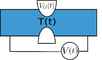
Figure 1: (Color online) A quantum point contact with time-dependent bias voltage $V(t)$ applied on the right lead. The transparency of the QPC, $T(t)$, is controlled by the gate voltage $V_{G}(t)$.Gershon et al. (2008)

The two Fermi seas are initially uncoupled. Usually it is assumed Muzykantskii and Adamov (2003) that the tunneling barrier is lowered at time $t=0$, allowing electrons to tunnel between the two leads, and is restored to fully reflective after a measurement time, $t_{f}$. In general, the evolution of outgoing states should be described by solving the fully time-dependent Hamiltonian $H(t)=H_{0}+H^{\prime}(t)$, with

$$H^{\prime}(t)=\sum_{j,j^{\prime}}\mathbf{c}_{j}^{\dagger}\mathbf{M}(t,\varepsilon_{j},\varepsilon_{j^{\prime}})\mathbf{c}_{j^{\prime}}.$$ (1)

The matrix $\mathbf{M}(t)=0$ for $t<0$ and $t>t_{f}$. However, if the scattering potential varies slowly on the scale of the Wigner delay time $\tau_{d}\ll\tau_{W}\sim S^{-1}\frac{\partial S}{\partial E}$, with $\hbar=e=1$, the properties of the system can be determined from the instantaneous value of scattering matrix $S(t)$ evaluated on states at the Fermi energy

$$S(t,E=\mu)=\left(\begin{array}[]{cc}B(t)&A(t)\\ -A^{\ast}(t)&B^{\ast}(t)\end{array}\right).$$ (2)

Here $A(t)$ and $B(t)$ are time-dependent transmission and reflection amplitudes and are determined by both the QPC gate voltage and the bias voltage applied between the leads. This relates eigenstates $c_{j}$ of $H_{0}$, which we separate into incoming $a_{j}$ and outgoing states $b_{j}$, via

$$\begin{pmatrix}b_{L}(t)\\ b_{R}(t)\end{pmatrix}=S(t)\begin{pmatrix}a_{L}\\ a_{R}\end{pmatrix}.$$ (3)

We are interested in the distribution $P_{n}$, which is the probability that there is a net transfer of $n$ charges from the left to the right lead during the measurement period $0<t<t_{f}$. A convenient way of characterizing the Full Counting Statistics (FCS), $P_{n}$, is via the function $\chi(\lambda)$:

$$\chi(\lambda)=\sum_{n=-\infty}^{\infty}P_{n}e^{i\lambda n}.$$ (4)

The current, noise and higher order cumulants, $\langle\langle Q^{m}\rangle\rangle$, can be computed from $\chi(\lambda)$: $\langle\langle Q^{m}\rangle\rangle=\frac{\partial^{m}\ln(\chi)}{\partial(i\lambda)^{m}}|_{\lambda=0}$, where $m$ is the order of the cumulant. The formula for the FCS is:Levitov and Lesovik (1993); Klich (2003); Muzykantskii and Adamov (2003)

$$\chi(\lambda)=\det(1+n(S^{\dagger}e^{i\lambda L}Se^{-i\lambda L}-1)),$$ (5)

where $n$ is the number operator for the fermions. The matrix $L$ projects onto states in the left lead: $\begin{pmatrix}1&0\\ 0&0\end{pmatrix}$ in lead space. The matrix inside the determinant is infinite dimensional in the energy or time domain and $2\times 2$ in lead space. Because of the infinite dimensionality of the space of states in (5), careful regularization of the formula is required. Klich (2003); Muzykantskii and Adamov (2003); Avron et al. (2007) For example, at very high energies $\varepsilon\rightarrow+\infty$, $n=0$, the argument of the determinant approaches the identity and the contributions remain finite and computable. However, when $\varepsilon\rightarrow-\infty$, $n=1$, and the matrix has the asymptotic form $S^{\dagger}e^{i\lambda L}Se^{-i\lambda L}$, which makes the determinant ill-defined for an infinitely deep Fermi sea.

A simple and correctly regularized approach to the computation of $\chi(\lambda)$ works with the density matrix for the outgoing states in one of the leads. The density matrices for incoming states in both leads can be written $n^{in}=\langle 0|a^{\dagger}_{j}a_{j}|0\rangle=n_{j}=\theta(\mu-\varepsilon_{j})$, which is the Fermi distribution function at zero temperature. Fourier transformed to the time domain, the density matrix has the form $n^{in}(t,t^{\prime})=\int d\varepsilon\theta(\mu-\varepsilon)e^{i(t-t^{\prime})(\varepsilon-\mu)}=\frac{i}{2\pi}\frac{1}{t-t^{\prime}+i0}$. The density matrix of the outgoing states in, say, the left lead $n^{out}(t,t^{\prime})$ can be obtained from (3):

$$n^{out}(t,t^{\prime}) = \langle b_{L}^{\dagger}(t)b_{L}(t^{\prime})\rangle$$ (6)

$$= B^{\ast}(t)n^{in}_{L}(t,t^{\prime})B(t^{\prime})+A^{\ast}(t)n^{in}_{R}(t,t^{\prime})A(t^{\prime}).$$

In the second equation, we have used the fact that terms like $\langle a^{\dagger}_{L}a_{R}\rangle$ are zero, because the incoming states between different leads are uncorrelated.

From $n^{out}$, it is possible to compute the cumulants directly. For example, the second cumulant (noise) is Lee and Levitov (1993)

$$\langle\langle Q^{2}\rangle\rangle = 2\iint dtdt^{\prime}n^{in}(t,t^{\prime})\left[1-n^{in}(t^{\prime},t)\right]$$ (7)

$$\left[|A(t)|^{2}|A(t^{\prime})|^{2}+A^{\ast}(t)B(t)A(t^{\prime})B^{\ast}(t^{\prime})\right].$$

In the case, when the barrier transparency is switched on and off with $A(t)=A_{0}=const$ for $0<t<t_{f}$ and $A(t)=0$ otherwise, and with no bias voltage applied between the leads, the so-called equilibrium noise is obtained from the integral in (7): $\langle\langle Q^{2}\rangle\rangle=\frac{A_{0}^{2}}{\pi^{2}}\log t_{f}\xi$. Here $\xi$ is the commonly used ultraviolet energy cut-off of the order of Fermi energy. The logarithmic term is present for almost all profiles and not just abrupt switching. It was found, for example, for the case of a Gaussian switching profile.Moskalets and Büttiker (2007)

The eigenvalues, $n_{j}$, of $n^{out}$ allow for the direct computation of the FCS. We consider first a simple case, where only one eigenvalue changes to $n_{j}$ and all other eigenvalues are unchanged. Since all eigenvalues initially are either 0 or 1, we need only to consider a change $0\rightarrow n_{j}$ or $1\rightarrow n_{j}$. In the first case, the probability of one additional particle being transferred into state $j$ from the right lead is $n_{j}$, while the probability, that no particle is added, $(1-n_{j})$. The counting statistics follow from (4) and are given by $\chi_{j}(\lambda)=1-n_{j}+e^{i\lambda}n_{j}$, with the average charge transfer given by $\langle Q\rangle=\frac{\partial\ln\chi}{\partial(i\lambda)}|_{\lambda=0}=n_{j}$. If the occupation changes from $1\rightarrow n_{j}$, a single hole is transferred with probability $1-n_{j}$ while no charge transfer takes place with probability $n_{j}$. For this case, $\chi_{j}(\lambda)=n_{j}+e^{-i\lambda}(1-n_{j})$, with the average charge transfer $\langle Q\rangle=n_{j}-1$. The results for the two cases can both be written

$$\chi_{j}(\lambda)=e^{i\lambda(\langle Q\rangle-n_{j})}[1+(e^{i\lambda}-1)n_{j}].$$ (8)

Since we work in the basis where $n^{out}$ is diagonal, the result for $\chi(\lambda)$ for the general case is simply a product over the factors, $\chi_{j}(\lambda)$. Taking account of all possible processes, we arrive at the formula Sherkunov et al. (2009); Abanov and Ivanov (2008); Klich (2003); Avron et al. (2007),

$$\chi(\lambda)=e^{i\lambda\langle Q\rangle}\prod_{j=1}^{N}e^{-i\lambda n_{j}}[1+(e^{i\lambda}-1)n_{j}].$$ (9)

It is correctly regularized as states unaffected by the perturbation contribute a factor $1$ to $\chi(\lambda)$. It is also well suited to direct numerical calculation.

In the following sections, we will discuss two special cases where the FCS can be obtained analytically. We rederive the known results for these cases by working directly with the density matrix, $n^{out}$. Then we show how the FCS for the general case are easy to obtain by diagonalizing $n^{out}$ numerically. To facilitate the interpretation of (9), we choose a specific form for the scattering matrix $S(t)$, and assume that the transmission and reflection amplitudes of the barrier $A(t)$ and $B(t)$ controlled by the QPC are real. If a bias voltage $V(t)$ is applied between the leads, its effect is to introduce an additional phase difference between the states in the two leads given by the Faraday flux $\psi(t)=\frac{e}{\hbar}\int_{0}^{t}V(t^{\prime})dt^{\prime}$. We incorporate this effect via a gauge transformation applied to states in the right lead: $a_{R}\rightarrow a_{R}e^{i\psi(t)}$. The resulting scattering matrix $S(t)$ is:

$$S(t)=\left(\begin{array}[]{cc}B(t)&A(t)e^{i\psi(t)}\\ -e^{-i\psi(t)}A(t)&B(t)\end{array}\right).$$ (10)

II.1 Bias-voltage applied between the leads

The case of a bias voltage pulse, $V(t)$, applied across a barrier with fixed transmission amplitude, $A$, for $0<t<t_{f}$ has been well studied. Levitov and Lesovik (1993); Levitov et al. (1996a); Ivanov et al. (1997) It has been shown that charge transfer processes at zero temperature are made up of combinations of two elementary events called uni-directional and bi-directional. Ivanov et al. (1997); Vanević et al. (2007) The uni-directional event relates to a single charge transfer process associated with the dc component of the bias voltage $V(t)$. A single state is occupied on one side of the barrier and not on the other. This leads to the possibility of the transfer of charge across the barrier but only in one direction. Unidirectional events contribute to the average current as well as higher order cumulants. Bi-directional events are the consequence of the ac component of $V(t)$, and relate to the excitation of equal numbers of particles and holes. These can both be transferred or reflected at the barrier so that charge can be transferred in either direction. No average current is generated in this case and only even cumulants are non-zero. The generic formula for the FCS for charge transfer is Vanević et al. (2007)

$$\chi(\lambda)=\prod_{i=1}^{N_{u}}(R+Te^{i\kappa\lambda})\prod_{j=1}^{N_{b}}[1+RT\sin^{2}\frac{\alpha_{j}}{2}(e^{i\lambda}+e^{-i\lambda}-2)].$$ (11)

$T=|A|^{2}$ is the barrier transparency and $R=1-T$. $N_{u}$ and $N_{b}$ correspond to the total number of uni- and bi-directional events. $\kappa=\pm 1$ depending on the polarity of the voltage pulse. The angles $\alpha_{j}/2$ determine the probability of exciting a single particle-hole pair in a bi-directional event. $N_{u}$, $N_{b}$ and $\alpha_{j}/2$ can be computedVanević et al. (2007) by diagonalizing matrix $h\tilde{h}$, where $h$ and $\tilde{h}$ are defined as $h=2n-1$ and $\tilde{h}=UhU^{\dagger}$, with $U(t)=e^{i\psi(t)}$.

We can understand the form of (11) by considering the density matrix of outgoing states, which in the case of constant transparency has the form

$$n^{out}(t,t^{\prime})=Rn^{in}_{L}(t,t^{\prime})+Te^{i\psi(t)}n^{in}_{R}(t,t^{\prime})e^{-i\psi(t^{\prime})}.$$ (12)

We assume that the measurement time is short enough that we can ignore the equilibrium noise contribution, which is a logarithmically divergent function of the measurement time $t_{f}$. Sherkunov et al. (2009) The equilibrium noise is associated with fluctuations in the number of particles in the left or right lead and occurs even in the absence of an applied voltage.

The dc component of the voltage pulse, associated with non-zero Faraday flux $\psi$, generates additional occupied particle (or hole) states in the right lead when compared with the incoming states in the left lead. The corresponding particle (or hole), after impinging on the barrier, will tunnel across with probability $T=A^{2}$ or be reflected with probability $R=1-T$. This gives rise to so-called uni-directional events. The eigenvalue of the density matrix for outgoing states in the left lead is then $n_{j}=T$, with an average charge transfer from right to left of $\langle Q\rangle=T$ if $j$ relates to a state above the Fermi energy, or $n_{j}=1-T$ and $\langle Q\rangle=-T$ if $j$ relates to a state below the Fermi energy. Inserting this in (9), gives $\chi_{u}(\lambda)=R+Te^{i\kappa\lambda}$, where $\kappa=\pm 1$ is determined by the type of transferred charge (particle or hole).

An example of unidirectional events is provided by the so-called minimal excitation states (MES). These excite a number of particles (or holes) with minimum noise. Ivanov et al. (1997); Keeling et al. (2006) The corresponding voltage pulse $V(t)$ is a sum of Lorentzian pulses: $V(t)=\sum_{j}^{N}\frac{2\tau_{j}}{(t-t_{j})^{2}+\tau_{j}^{2}}$, where $t_{j}$ and $|\tau_{j}|$ determine the center and width of the $j$th pulse respectively. The unitary transformation in (10) is

$$e^{i\psi(t)}=\prod_{j}^{N}\frac{t-t_{j}-i\tau_{j}}{t-t_{j}+i\tau_{j}}.$$ (13)

Choosing the signs of the $\tau_{j}$ to be the same leads to $N$ unidirectional events. For $N=1$, the pulse in (13) generates a single uni-directional event with one particle (electron or hole, depending on the polarity of the pulse) passing through the barrier with probability $T$ giving $\chi(\lambda)=R+Te^{ik\lambda}$. For $N=2$, with the polarities of the two pulses (set by the signs of the $\tau_{j}$) the same, the two uni-directional events are combined and $\chi(\lambda)=(R+Te^{i\kappa\lambda})^{2}$ irrespective of the relative widths ($|\tau_{j}|$) or positions ($t_{j}$).

The ac component of the voltage pulse, associated with zero total Faraday flux, gives rise to the so-called bi-directional events—the simplest example of which is given by a pulse of the type (13) with $N=2$ and $\tau_{1}\tau_{2}<0$. The operator $h\tilde{h}$ characterizes the differences between the states in the two leads following the application of the pulse. All states, which are either both occupied or both empty in the two leads and which therefore contribute a factor 1 to $\chi(\lambda)$, are eigen states of $h\tilde{h}$ with eigenvalue 1 ($\alpha_{j}=0$). All other eigenvalues occur in pairs and are equal to $e^{\pm i\alpha_{j}}$. Vanević et al. (2007) In the basis of the unperturbed states of either of the leads, the state described by $\tilde{h}$ contains an admixture of the unperturbed state and independent particle and hole excitations in each of the $2$ dimensional subspaces of the basis (labeled by $j$), in which $\tilde{h}$ is block diagonal. Its eigenvalues are $e^{\pm i\alpha_{j}}$. Each of these will lead to eigenvalues in $n^{out}$ of $n_{j}$ and $(1-n_{j})$, one associated with the particle excitation and one with the hole.

The contribution to $\chi(\lambda)$ from each of these bi-directional events (corresponding to the different $j$) is the product over the two factors of the type in (8), one with eigenvalue $n_{j}$ ($\langle Q\rangle=n_{j}$) and one with eigenvalue $1-n_{j}$ ($\langle Q\rangle=n_{j}-1$): $\chi_{b}(\lambda)=\left(1+(e^{i\lambda}-1)n_{j}\right)\times\left(1+(e^{-i\lambda}-1)(1-n_{j})\right)=1+n_{j}(1-n_{j})(e^{i\lambda}+e^{-i\lambda}-2)$. To make a connection between $n_{j}$ and rotation angle $\alpha_{j}/2$, we use the known resultVanević et al. (2007) $h=\begin{pmatrix}0&1\\ 1&0\end{pmatrix}$ and $\tilde{h}=\begin{pmatrix}0&e^{-i\alpha_{j}}\\ e^{i\alpha_{j}}&0\end{pmatrix}$ in the eigenbasis of $h\tilde{h}$. Substituting $h$ and $\tilde{h}$ into (12) and diagonalizing $n^{out}$ explicitly, we obtain $n_{j}=\frac{1}{2}\pm\frac{1}{2}\sqrt{1-4RT\sin^{2}\frac{\alpha_{j}}{2}}$ and

$$n_{j}(1-n_{j})=RT\sin^{2}\frac{\alpha_{j}}{2}.$$ (14)

After taking the product over all events labeled by $j$, and adding in the contribution of the uni-directional events, we recover (11). For a given voltage pulse between the leads and corresponding unitary transformation $U(t)$, the $\alpha_{j}/2$ can be thought of as the rotation angles of the ground state associated with $U(t)$ and are found by diagonalizing the $h\tilde{h}$. Vanević et al. (2007); Sherkunov et al. (2008) The rotated state is an admixture of the original state, with probability $\cos^{2}\frac{\alpha_{j}}{2}$, and the state with an added particle and hole, with probability $\sin^{2}\frac{\alpha_{j}}{2}$. The factor $1+RT\sin^{2}\frac{\alpha_{j}}{2}(e^{i\lambda}+e^{-i\lambda}-2)$ is the weighted average of the result for the unperturbed state (contribution 1 with weight $\cos^{2}\frac{\alpha_{j}}{2}$) and for the state with an added particle and hole (contribution $(R+Te^{i\lambda})(R+Te^{-i\lambda})$ with weight $\sin^{2}\frac{\alpha_{j}}{2}$).Sherkunov et al. (2008)

II.2 Barrier with modulated Transparency

Another case for which results in closed form have been reported is that of a time-dependent barrier between two leads at the same chemical potential. Andreev and Kamenev (2000); Sherkunov et al. (2009) The problem can be mapped onto a special case of a voltage biased time-independent barrier with constant transmission and reflection amplitudes. Sherkunov et al. (2009) This mapping becomes explicit once the problem is approached via the density matrix of the outgoing states. In the absence of a bias the scattering matrix in (10) simplifies to $S(t)=\left(\begin{array}[]{cc}B(t)&A(t)\\ -A(t)&B(t)\end{array}\right)$ and the density matrix of outgoing states becomes $n^{out}(t,t^{\prime})=B(t)n(t,t^{\prime})B(t^{\prime})+A(t)n(t,t^{\prime})A(t^{\prime})$. Introducing $e^{i\phi(t)}=B(t)+iA(t)$ (we are still assuming that $A$ and $B$ are real), we insert $e^{i\phi(t)}$ into $n^{out}$ and eliminate $A$ and $B$. We obtain $n^{out}=\frac{1}{2}(e^{i\phi}n^{in}e^{-i\phi}+e^{-i\phi}n^{in}e^{i\phi})$. Here we have used the fact that $n^{in}_{L}=n^{in}_{R}=n^{in}$.

Since a unitary transformation on $n^{out}$ does not affect its eigenvalues, $n_{j}$, we can study

$$e^{-i\phi}n^{out}(t,t^{\prime})e^{i\phi}=\frac{1}{2}n^{in}(t,t^{\prime})+\frac{1}{2}e^{2i\phi(t)}n^{in}(t,t^{\prime})e^{-2i\phi(t^{\prime})}.$$ (15)

The relations (15) and (12) have the same structure. The FCS of a system with modulated barrier transparency without a bias between the leads are therefore equivalent to those for a system with bias voltage applied across a barrier with constant transmission and reflection amplitudes $A=B=\frac{1}{\sqrt{2}}$, and Faraday flux $\psi=2\phi$. The FCS for a modulated barrier transparency can therefore be obtained from (11). In addition, other concepts developed to understand the bias voltage case carry over to the modulated barrier case. These include the geometrical interpretation of the FCS, Sherkunov et al. (2008) as well as the MES, Keeling et al. (2006) which, when implemented as a modulation profile of the barrier leads to the optimal entangler of electron hole pairs.Sherkunov et al. (2009)

To calculate $\chi(\lambda)$ for the case of the modulated barrier from (11), we need, as before, to diagonalize the matrix $h\tilde{h}=he^{2i\phi}he^{-2i\phi}$ and compute the angles $\alpha_{j}/2$ from its eigenvalues. Since no bias voltage is applied between the leads, the system is completely symmetric in lead space. As a result only bi-directional events (leading to no net average charge transfer) can occur and all the eigenvalues of $he^{2i\phi}he^{-2i\phi}$ come in pairs. The characteristic function $\chi(\lambda)$ is then given by

$$\chi(\lambda) = \prod_{j=1}^{N}\left(1+\frac{1}{4}\sin^{2}\frac{\alpha_{j}}{2}(e^{i\lambda}+e^{-i\lambda}-2)\right)$$ (16)

$$= \prod_{j=1}^{N}\left(1-\sin^{2}\frac{\alpha_{j}}{2}\sin^{2}\frac{\lambda}{2}\right),$$

where $N$ is the number of paired eigenvalues determined from $he^{2i\phi}he^{-2i\phi}$.

To illustrate the value of this mapping, consider the case in which the transparency of a barrier is subjected to a sinusoidal modulation: $A(t)=\sin\omega t$ and $B(t)=\cos\omega t$. If the total number of cycles is large enough, the contribution from the equilibrium noise (proportional to $\log t_{f}\xi$) can be neglected. This problem can be mapped to a case of a barrier with constant bias voltage with transparency $T=1/2$ and $\psi=\int^{t}V(t^{\prime})dt^{\prime}=2\phi=2\omega t$ corresponding to a constant dc bias with $V=2\omega$.

To obtain the FCS, we need to diagonalize matrix $he^{2i\omega t}he^{-2i\omega t^{\prime}}$. As this corresponds to a constant dc bias problem involving two uni-directional events per period, (the phase changes by $4\pi$ per period), there are two eigenvalues different from 1 and both are equal to -1. The polarity (particle or hole) of transferred charge can be inferred from the requirement that there is no net average charge transfer. Hence we conclude that the sinusoidally modulated transparency case is equivalent to one electron and one hole impinging in a single period on a barrier with transmission $T=1/2$. The two processes are independent since both correspond to uni-directional events in the equivalent bias voltage problem. The FCS for constant bias voltage case are known to be given by $\chi_{0}(V,\lambda)=(R+Te^{i\kappa\lambda})^{\frac{t_{f}V}{4\pi}}$, with $\kappa=\pm 1$ depending on the polarity of the applied voltage. Lee and Levitov (1993); Muzykantskii and Adamov (2003) The corresponding FCS for the sinusoidally modulated transparency case is a combination of two factors $\chi_{0}$ one with $\kappa=1$ and one with $\kappa=-1$. This gives

$$\chi(\lambda) = \chi_{0}(\omega,\lambda)\chi_{0}(\omega,-\lambda)$$ (17)

$$= \left(\frac{1+\cos\lambda}{2}\right)^{\frac{\omega t_{f}}{2\pi}},$$

which is a result previously obtained by Andreev and Kamenev using the Keldysh formalism. Andreev and Kamenev (2000) A barrier operated in this way acts as a quantum pump which excites exactly one electron-hole pair per period, provided the logarithmically divergent equilibrium noise is neglected. The four possible outcomes per cycle are shown in Fig. 2.

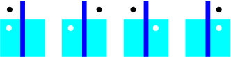
Figure 2: (Color online) Four possible outcomes per period from a sinusoidally modulated barrier transparency. All four outcomes are equally likely. The particle-hole pair can be on either side of the barrier or as an entangled pair of particle on one side and hole on the other.

The result (17) is the ac version of the barrier profile required to generate optimal electron entanglement. Sherkunov et al. (2009) The profile

$$e^{i\phi(t)}=B(t)+iA(t)=\frac{t-i\tau}{t+i\tau}$$ (18)

generates the FCS $\chi(\lambda)=(1+\cos\lambda)/2$. The use of a quantized Lorentzian pulse of the type (18) has the advantage that the equilibrium noise is strictly absent in (18). Although the entanglement generated by (18) is between electrons and holes and therefore not useful in quantum computation due to the charge conservation laws,Klich and Levitov the protocol would be useful if combined with another degree of freedom (either spin or orbital) because it operates in a one-shot mode. The difficulty with its operation is associated with the precise generation of the actual profile. We explore the effect of possible errors in its experimental implementation in Sec.III.2.

II.3 Fermi Edge Singularity

We discuss here the relation between the FCS of a contact subjected to sharp bias voltage pulses and the Fermi Edge Singularity (FES). We map to the problem of an unbiased contact for which the result for the FCS is known.

We consider two delta pulses with opposite signs separated by $t_{f}$ applied to one lead. The contact has fixed transparency $T$ and reflectance $R$. The corresponding voltage profile is

$$V(t)=\frac{\psi}{2\pi}[\delta(t)-\delta(t-t_{f})],$$ (19)

with $\psi=const$. This pulse induces a phase shift $\psi$ on the incoming states of, say, the left lead (measured with respect to the right one) within time window $0<t<t_{f}$ and zero phase shift otherwise. For $\psi\gg 2\pi$ and large $t_{f}\xi$, the noise can be written as an expansion in $(\xi t_{f})^{-1}$

$$\langle\langle Q^{2}\rangle\rangle=2RT[\frac{2}{\pi^{2}}\sin^{2}\frac{\psi}{2}\ln t_{f}\xi+\frac{\psi}{2\pi}]+\cdots.$$ (20)

The derivation of (20) is essentially the same as that given by Lee and Levitov (LL) for the quantum current fluctuations induced by a magnetic field in a metallic loop containing a QPC.Lee and Levitov (1993) The FCS for the problem we are considering have been computedSherkunov et al. (2008) but only for the case that the transparency of the barrier is low. In this section we address the general problem with arbitrary contact transparency.

As the two electrodes are equivalent, only bi-directional events occur in this problem. By (11), the counting statistics are

$$\chi(\lambda)=\prod_{j}[1-\sin^{2}\frac{\alpha_{j}}{2}\sin^{2}\frac{\tilde{\lambda}}{2}],$$ (21)

where we have defined $\sin\frac{\tilde{\lambda}}{2}=2\sqrt{RT}\sin\frac{\lambda}{2}$. The central problem is how to compute angles $\frac{\alpha_{j}}{2}$. Eq. (21) has the same form as (16), which is that for a barrier with time-dependent reflection and transmission amplitudes $B(t)+iA(t)=e^{i\psi(t)/2}$. For $0<t<t_{f}$, $A(t)=\sin\frac{\psi}{2}=const$ and $A(t)=0$ if $t<0$ or $t>t_{f}$. One interesting complication in this problem is that the FCS are only well-defined if the limit of increasingly sharp voltage profiles, $V(t)$, leading to the delta functions in (19), is specified. This is because the shape of the voltage pulse, leading to the Faraday flux change from zero to $\psi$, affects the number of excitations introduced by the switching process. In the mapped barrier opening problem, the precise time-dependence of the (rapid) opening and closing of the barrier matters. An example of a possible profile for this opening of the barrier is shown Fig. 3.

For the case that the barrier switching time $\tau$ is very short compared to the measurement time $t_{f}$, we argue that the switching processes, which excites high energy ($\sim 1/\tau$) particle-hole pairs, should not interfere with the long time measurement process, which leads to the low energy excitations, predominantly on the energy scale $\sim 1/t_{f}$, expected for a Fermi Edge Singularity problem. We make the Ansatz that the FCS can be written as a product of the types of processes as

$$\chi(\lambda)=\chi_{1}(\lambda)\chi_{2}(\lambda),$$ (22)

with $\chi_{2}$ giving the FES contributions (which are associated with the shaded region, shown schematically as the shaded area in Fig. 3). $\chi_{1}$ gives the contribution associated with the opening profile at $t=0$ and $t_{f}$. We focus here on the calculation of $\chi_{2}$ and postpone the computation of $\chi_{1}$ to Sec. III.2 where numerical techniques are adopted.

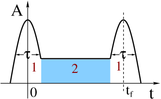
Figure 3: (Color online) Illustrative transmission amplitude $A(t)$ as a function of time $t$ for the the pulsed lead case after mapping to the equivalent barrier opening problem. The FCS are only well-defined if the exact time-dependence, whose limit is the delta function in (19), is specified. Here we show a case where the amplitude, $A(t)$, actually overshoots the value $\sin(\psi/2)$. We argue that the FCS should be well approximated by a product over two independent contributions from the two regions denoted by $1$ and $2$ (shaded region).

The FCS of an unbiased barrier, for which the reflection amplitude is abruptly changed from zero to the constant value $\sin\frac{\psi}{2}$ for a duration $t_{f}$, is known and was computed using the bosonization technique. Levitov et al. (1996b) The result can also be found by solving a Riemann-Hilbert problem Klich and Levitov (2009) valid even at non-zero temperature in Appendix B. The FCS is

$$\chi_{2}(\lambda)=\exp(-\lambda^{2}_{\ast}G),$$ (23)

with $G$ and $\lambda_{\ast}$ being given by

$$\sin\frac{\lambda_{\ast}}{2} = \sin\frac{\psi}{2}\sin\frac{\tilde{\lambda}}{2}=2\sqrt{RT}\sin\frac{\psi}{2}\sin\frac{\lambda}{2}$$ (24)

$$G = \frac{1}{2\pi^{2}}\ln t_{f}\xi.$$ (25)

The logarithmic terms in (20) are connected with the Fermi Edge Singularity found in metals.Mahan (1967); Nozieres and De Dominicis (1969) It is interesting to note that the form (24) includes the well-known result for the Anderson orthogonality catastrophe problem in a single lead Anderson (1967) as a special case. The quantity of interest is the overlap $\langle 0|0^{\prime}\rangle$ between $|0\rangle$, the ground state of an unperturbed metal and $|0^{\prime}\rangle$, the wavefunction of the same metal at a time $t_{f}$ after switching on a (core hole) potential. In the simplest case, the potential can be well described by a single energy-independent phase shift which is exactly equivalent to the phase $\psi$, with $e^{i\psi/2}=B+iA$ associated with the modulated barrier we have been considering. The overlap can be written as $\langle 0|0^{\prime}\rangle=\langle 0|e^{i\psi(t)}|0\rangle=\prod_{j}\cos\frac{\alpha_{j}}{2}$, where the $\frac{\alpha_{j}}{2}$ are the eigenvalues $e^{\pm\alpha_{j}}$ of $he^{i\psi/2}he^{-i\psi/2}$. This is equal to $\sqrt{\chi_{2}(\lambda=\pi,T=\frac{1}{2})}$. With $\lambda=\pi,T=\frac{1}{2}$, $\lambda_{*}=\psi$ and we recover Anderson’s result Anderson (1967): $\langle 0|e^{i\psi(t)}|0\rangle=(\xi t_{f})^{-\psi^{2}/(4\pi^{2})}$.

III General Case

In the general case, which is equivalent to having both a bias voltage between the leads and a time-dependent profile for the barrier, we are not aware of the existence of a simple relation mapping the problem onto an equivalent bias voltage problem. However, (9) allows for the calculation of the FCS as long as the spectrum of the density matrix of outgoing states is available.Abanov and Ivanov (2008) We can diagonalize $n^{out}$ in (6) numerically to find the eigenvalues $n_{j}$ and use (9) to compute the FCS.

Numerically, it is convenient to work in the energy domain with a discrete energy spectrum. (An alternative is to compute the dynamics of the system directly. For a finite system the spectrum is then automatically truncated and the determinant is properly regularizedSchönhammer (2007, ).) We introduce a periodic boundary condition in time, with period $t_{p}$, discretizing the energy spectrum of the scattering matrix with an energy separation $\omega_{0}=2\pi/t_{p}$. By choosing $t_{p}\ll t_{f}$ we can compute the counting statistics with large number of cycles, giving the characteristic function as $\chi(\lambda)\approx[\chi_{0}(\lambda)]^{t_{f}/t_{p}}$, where $\chi_{0}(\lambda)$ is the FCS for single period. We can also set $t_{p}\gg t_{f}$ and study the behavior of a device when operated in one-shot mode.

Fourier transformed into the energy domain, the individual matrix elements of $A(t)$ and $B(t)$ are $\mathbf{X}_{mn}=\frac{1}{t_{p}}\int_{0}^{t_{p}}e^{-i(m-n)\omega_{0}t}X(t)dt$ where $X$ stands for $A$ or $B$. The neighboring rows of $X_{mn}$ have the same elements though they are shifted from each other by one column. If $X(t)$ is sufficiently smooth, by which we mean its Fourier transform decays faster than $\omega_{0}^{\nu}$, with $\nu<-1$. We can cut off the Fourier series and limit the approximated summation within $|m-n|<M$ with $M$ chosen large enough to achieve the desired accuracy. The truncated matrices $\mathbf{A}$ and $\mathbf{B}$ are blockwise tridiagonal with each block size $M\times M$. After some manipulation, the diagonalization of the infinite dimensional matrix $n^{out}$ is approximately equivalent to the diagonalization of a $2M$ dimensional matrix in energy space. Details of this procedure are summarized in App. A.

In this section, we look at cases where the direct diagonalization of the matrix $n^{out}$ allows the study of the FCS of a tunnel barrier with time-dependent scattering amplitudes with a bias voltage applied between the leads. We concentrate, in particular, on the example of a barrier used as a low noise source and study how the noise and degree of entanglement are affected by deviations from the optimal pulses which have been proposed.Sherkunov et al. (2009); Keeling et al. (2008) Mostly, we will study barrier and voltage profiles which are either combinations (or close to combinations) of the quantized Lorentzian pulses. These can be applied as voltage pulses to a lead with (13) describing the corresponding Faraday flux $e^{i\psi(t)}$, or with (13) describing the barrier profile $e^{i\phi(t)}=B(t)+iA(t)$.

III.1 Quantized Pulses

To operate a tunneling barrier as a single electron source at low temperatures requires a voltage pulse which excites a single electron excitation in one lead. This can be achieved by creating a MES with a single Lorentzian pulse applied between the leads. At low temperatures, the noise produced by such a device comes from two sources: shot and equilibrium noise. Blanter and Buttiker (2000) The shot noise for the simplest case of a barrier with constant transmission probability, $T$, is proportional to $T(1-T)$ for a single MES pulse. This suggests that one should aim to open the barrier fully ($T=1$) to increase the chance of single electron emission. However, if we open the barrier in an arbitrary way, the equilibrium noise becomes important. A solution Sherkunov et al. (2009) is to combine the creation of the MES, choosing a bias voltage pulse giving Faraday flux

$$e^{i\psi(t)}=\frac{t-t_{0}-i\tau_{0}}{t-t_{0}+i\tau_{0}}$$ (26)

in the incoming states, with a carefully-chosen opening profile for the barrier which minimizes the total noise.

Since the profile generating the maximal entanglement (18), as illustrated in Fig. 4(a), fully opens the barrier twice without any equilibrium noise contribution depending logarithmically on $t_{f}$, a first guess is that it might also work as a possible profile for the opening of the barrier when used as a single electron source. However, the barrier opening scheme based on (18) is not ideal for a single electron emission. Though the logarithmic term in the equilibrium noise is absent, the profile does generate background noise with (see 16) $\langle\langle Q^{2}\rangle\rangle_{0}=\frac{\partial^{2}\log\chi}{\partial(i\lambda)^{2}}=\sum_{j}^{N}\frac{1}{2}\sin^{2}\frac{\alpha_{j}}{2}\leq\frac{N}{2}$. For the profile (18) and $N=1$ and $\alpha=\pi$ we find $\langle\langle Q^{2}\rangle\rangle=\frac{1}{2}$ which is actually the maximum for a single pulse.

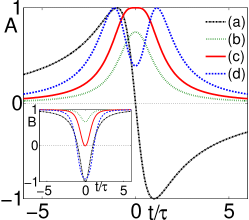
Figure 4: (Color online) Transmission coefficients $A(t)$ for some opening profiles for a barrier. The centers of the pulses are at $t=0$, with time scaled in units of the pulse width $\tau$. (a) Single Lorentzian pulse (see 18) for optimal entangler. (b) Two Lorentzian pulses, with opposite polarities (see 27) with $\tau_{1}=\tau_{2}=\tau$ and pulse separation $t_{1}/\tau\approx 0.6$. (c) Same as in (b) with separation $t_{1}/\tau\approx 0.83$ (optimal). (d) Same as in (b) with $t_{1}/\tau\approx 1.2$. The inset shows the corresponding reflection amplitude $B$ as a function of $t/\tau$. Only in cases (b) and (c) do both $A$ and $B$ remain positive during the pulse lifetime.

We consider instead a pair of such pulses:

$$e^{i\phi(t)}=\frac{t-t_{1}/2-i\tau_{1}}{t-t_{1}/2+i\tau_{1}}\frac{t+t_{1}/2+i\tau_{2}}{t+t_{1}/2-i\tau_{2}},$$ (27)

where the separation of the two pulses (with widths $\tau_{1}$ and $\tau_{2}$ respectively) is $t_{1}$. A little algebra shows that $A(t)$ and $B(t)$ do not change sign only if $\tau_{1}=\tau_{2}$ and $\tau_{1}/t_{1}\geq\frac{1}{2}+\frac{1}{\sqrt{2}}$. Corresponding typical profiles are shown in Fig. 4(b-c). The ratio $\tau_{1}/t_{1}=\frac{1}{2}+\frac{1}{\sqrt{2}}$ gives a transparency of the barrier which has a single maximum with $A=1$ at $t=0$, as shown in Fig. 4(c). We have found empirically that this separation gives the best combination (low total noise and highest probability for the transfer of one electron). Exciting a single excitation in the incoming states of one lead and coordinating the timing of this excitation with the opening of the barrier, allows the single particle excitation in the incoming states to impinge upon the barrier when it is fully open. An advantage of the profile (27) is that, owing to cancelation between the two components (at $t=-t_{1}/2$ and $t=t_{1}/2$) at long times, the transmission amplitude $A(t)$ approaches zero faster than for the profile (18). In addition, the noise generated by this opening profile $\langle\langle Q^{2}\rangle\rangle_{0}\approx 0.23$, which is less than half that generated by (18). We expect that the profile (27), with an optimally chosen ratio for $t_{1}/\tau_{1}$, should be a good candidate for designing an on-demand single electron source at ultralow temperatures.

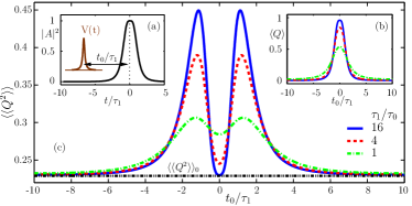
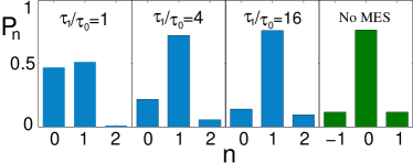
Figure 5: (Color online) Upper panel: Single unidirectional event in a quantum contact with tunable transparency (numerical calculations). (a) Transparency of the barrier as a function of time given by (27). We also show an MES applied to a lead (26). (b) Average charge transfer $\langle Q\rangle$ between the two leads as a function of $t_{0}$. The maximum of $\langle Q\rangle$ is around $0.96$ for the narrowest MES considered $\tau_{1}/\tau_{0}=16$. (c) Noise in a biased contact with transparency (27) as a function of $t_{0}/\tau_{1}$. The minimal value of the noise corresponds to $t_{0}=0$ and, for the narrowest MES pulse ($\tau_{1}/\tau_{0}=16$), it almost drops to the value due to barrier modulation: $\langle\langle Q^{2}\rangle\rangle_{{}_{0}}$ (dotted line). The two maxima in the noise occur when $t_{0}/\tau_{1}\approx 1$ and the transparency is almost $1/2$. Lower panel: Probability distribution $P_{n}$ for $\tau_{1}/\tau_{0}=1$,$4$ and $16$ at $t_{0}=0$, as well as the probability distribution generated by profile (27) only without the MES applied on the lead. We see that in the limit $\tau_{1}/\tau_{0}\rightarrow\infty$, $P_{n}$ approaches $P^{0}_{n\pm 1}$. (See text)

For $\tau_{1}/t_{1}=\frac{1}{2}+\frac{1}{\sqrt{2}}$ and with a single pulse $e^{i\psi}=\frac{t-t_{0}-i\tau_{0}}{t-t_{0}+i\tau_{0}}$ applied to the lead, we have diagonalized the density matrix $n_{out}$ numerically. Fig. 5(a) shows results for the noise $\langle\langle Q^{2}\rangle\rangle$ in the system as a function of the separation $t_{0}$ between the center of the MES pulse and the maximum of barrier transparency (for which $A=1$ at $t=0$). The maximum values of the noise occurs when $t_{0}\approx\tau_{1}$ and the transparency coefficient is almost $1/2$. This is the regime where the barrier is acting as a $50\%$ beam-splitter. The minimum of $\langle\langle Q^{2}\rangle\rangle$ corresponds to $t_{0}=0$, when $|A|^{2}=1$. At $t_{0}=0$ the transferred charge as well as the quality factor $\langle Q\rangle/\langle\langle Q^{2}\rangle\rangle$ attains its maximum. Fig. 5(b) shows the average transferred charge $\langle Q\rangle$ as a function of $t_{0}$. If the pulse applied to the lead is narrow compared to the opening time of the barrier ($\tau_{0}\ll\tau_{1}$), the minimum value of the noise is essentially set by the noise associated with the opening of the barrier, namely $\langle\langle Q^{2}\rangle\rangle_{{}_{0}}$. The transferred charge approaches $1$ when $\tau_{0}/\tau_{1}\rightarrow 0$ and the probability distribution for transferred charge, $P_{n}$, approaches $P^{0}_{n\pm 1}$ (the sign depends on the polarity of the voltage pulse applied to the incoming states in one of the leads) is shown in the lower panel in Fig 5. Here $P^{0}_{n\pm 1}$ is the probability distribution for charge transfer associated with the opening of the barrier without a bias pulse applied between the leads.

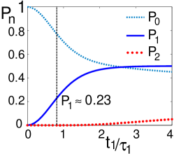
Figure 6: (color online) Evolution of the probability for electron-hole pair emission as a function of pulse separation $t_{1}/\tau_{1}$ for a barrier profile (27) with $\tau_{2}=\tau_{1}$. The dashed line gives the probability that nothing happens ($P_{0}$). The solid line is the probability of generating a single entangled electron-hole pair ($P_{1}$). The dotted line show the probability for two particle-hole pair emission ($P_{2}$). The vertical cut is the position where the single electron source profile (27) operates.

Fig 5 shows that, when $\tau_{1}/\tau_{0}=1$, the emission of 2 electrons is strongly suppressed. If it was important to have a source which only emitted single electrons and there was a method for discarding ‘non-events’ in which no electron was emitted, this protocol would work well. The suppression of double electron emission can be understood as follows. The width of pulse determines the energy profile of the excited particles or holes. When $\tau_{0}\sim\tau_{1}$, the particle excitation induced by the changing barrier profile has the same energy profile as that of the incoming excitation induced by the bias voltage applied between the leads. As the two pulses are coincident in time the Pauli exclusion principle leads to destructive interference between the two excitations in one lead and either only one particle or no particle will be transmitted through the QPC as a result.

The profile (27) does not involve a change of sign of either $A(t)$ or $B(t)$ and, consequently, should be easier to implement experimentally than the profile (18). We therefore consider how well the profile (27) might work as a (non-optimal) electronic entangler. Fig. 6 shows the probability of electron-hole pair production $P_{n}$ versus pulse separation $t_{1}/\tau_{1}$. The vertical line corresponds to $t_{1}/\tau_{1}=1/(\frac{1}{2}+\frac{1}{\sqrt{2}})\approx 0.83$, beyond which a sign change in $A(t)$ is necessary and the experimental implementation is expected to be more involved. We see that the emission of two electron-hole pairs is very unlikely. The only two significant outcomes are: no excitation, created with probability $P_{0}$, and the creation of a single (entangled) electron hole pair which is created with probability $P_{1}$. The corresponding entanglement entropy at this point is $S=P_{1}S_{Bell}\approx 0.23$, ie just under half the theoretical maximum.

III.2 Non-Quantized Pulses

So far, we have discussed (combinations of) quantized Lorentzian pulses applied to a lead (see 13) and/or barrier opening profiles (see 27) that excite a bounded number of electron-hole pairs without the accompanying equilibrium noise which grows logarithmically with $t_{0}$. Here, we focus on the increased noise resulting from deviations from the ideal quantized pulses.

We consider the case of a modulated barrier, with the following non-quantized opening profile:

$$B(t)+iA(t)=e^{i\phi(t)}=\left(\frac{t-i\tau_{1}}{t+i\tau_{1}}\right)^{\gamma_{1}}\left(\frac{t-t_{0}-i\tau_{2}}{t-t_{0}+i\tau_{2}}\right)^{\gamma_{2}}.$$ (28)

where $\gamma_{1,2}\in\mathbb{R}$. We look at the simplest case $\gamma_{2}=1-\gamma_{1}$ and $\gamma_{2}=-\gamma_{1}$ and choose $\tau_{1}=\tau_{2}=\tau$. In both cases $t_{0}$ plays the role of the measurement time $t_{f}$, provided $t_{0}\gg\tau$. The profile (28) with $t_{0}\gg\tau$ describes a barrier with a transmission amplitude, $A$, which changes from $0$ to $\sin 2\pi\gamma$ within a period of $\tau$ around $t=0$ and closes at $t=t_{0}$. There will then be a contribution to the noise which increases logarithmically with $t_{0}$ (this is just the equilibrium noise contribution). The mapping between the case of a barrier profile and a voltage bias across a junction with constant transparency means that this profile also models non-quantized voltage pulses applied between the leads. This mapping includes a doubling of the total phase change $2\phi=\psi$ (see Sec. II.2), which means that (28) describes two voltage pulses with Faraday flux $4\pi\gamma_{1,2}$. If the $\gamma_{i}$ are not both integer or half-integer, there is a net phase shift of $2\pi\gamma_{1}$ and $2\pi(\gamma_{1}+\gamma_{2})$ between the rotated and the unperturbed states with consequent FES effects.

The FCS for the profile (18), which gives the optimum level of entanglement, are equivalent to those for two quantized Lorentzian pulses, when the problem is mapped to the case of a junction with a bias, because of the associated doubling of the phase $2\phi=\psi$, This suggests that the pulse (18) applied to the barrier may be a special case of two separate pulses, each of which corresponds to a single quantized pulse in the case of a bias between the leads. In particular, a pulse

$$e^{i\phi(t)}=\left(\frac{t-i\tau_{1}}{t+i\tau_{1}}\right)^{\frac{1}{2}}\left(\frac{t-t_{0}-i\tau_{2}}{t-t_{0}+i\tau_{2}}\right)^{\frac{1}{2}},$$ (29)

consists of two pulses centered at $0$ and $t_{0}$ with widths $\tau_{1}$ and $\tau_{2}$. The absence of a logarithmic contribution to the noise in this case should be expected, because the barrier is closed at all times except for a period $\tau$ around $0$ and $t_{0}$. The effect of pulses (29) on the states of the system can be found by working in the basis in which the scattering matrix in (10) is diagonal. With $A$ and $B$ both real ($\psi=0$ as there is no applied bias), the scattering matrix is diagonal for all times in the basis $c_{1,2}=(c_{L}\pm ic_{R})/\sqrt{2}$ and its eigenvalues as a function of time are given by the values of $e^{\pm i\phi(t)}$ in (29). The two components of the pulse centered on $t=0$ and $t=t_{0}$ induce phase shifts of $\pm\pi$ in each channel and are individually as far as possible from quantized pulses. However their effect on the FCS of the charge transfer between the left and right leads depends only on the difference in phase shift between the two channels and each of the two components therefore contribute to the FCS as quantized pulses.

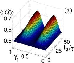
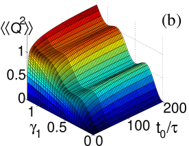
Figure 7: (Color online) The noise produced in the charge transfer across an unbiased barrier when its profile is varied according to (28). Results are shown as a function of the separation, $t_{0}/\tau$, between the two non-quantized pulses at $t=0$ and $t=t_{0}$, and of the exponent $\gamma_{1}$ with (a) $\gamma_{2}=1-\gamma_{1}$ and (b) $\gamma_{2}=-\gamma_{1}$. In case (a) the values $\gamma_{1}=0.5$ and $\gamma_{1}=1$ correspond to quantized pulses (when mapped to the problem of a biased lead, there is a doubling of the total phase change). The noise for all other values of $\gamma_{1}$ increases logarithmically with $t_{0}$. This is the equilibrium noise contribution. In case (b) the noise $\gamma_{1}=0.5$ and $\gamma_{1}=1$ saturates when the pulse separation $t_{0}$ is much larger than the pulse widths $\tau$. For all other $\gamma_{1}$ there is again the equilibrium noise contribution which grows logarithmically with measurement time $t_{0}$.

The noise generated by the opening profile (28) with $\tau_{1}=\tau_{2}=\tau$ is shown in Fig. 7(a) for the case $\gamma_{2}=1-\gamma_{1}$ and in Fig. 7(b) for the case $\gamma_{2}=-\gamma_{1}$. In both these cases the penalty for missing quantization of the pulses is small. The increase in noise at fixed $t_{0}$, as $\gamma_{1}$ deviates from integer or half-integer values, is slow. (For example, with $\gamma_{1}=1/2$ and $t_{0}/\tau=50$, a $10$% deviation in $\gamma_{1}$ introduces additional noise of only of $2$% of the quantized value.) This suggests that any reasonable experimental implementation of such pulses should allow the exploitation we have described (as entanglers or as electron sources). Case (a) corresponds to two Lorentzian (non-quantized) pulses with the same polarity separated by a time $t_{0}$. There are two peaks, the height of which grow logarithmically with $t_{0}$, with a flat valley in between. When $\gamma_{1}=1/2$ the profile is that of (29), and we find, as expected, results equivalent to the profile (18), ie a total noise equal to 1/2 and independent of $t_{0}$. For other values of $\gamma_{1}$ the noise grows with a logarithmic dependence on $t_{0}$. When $\tau<t_{0}$, the problem is that of two equivalent FES problems: The effect of the first pulse is to give rise to scattering phase shifts of $2\pi\gamma_{1}$ and $-2\pi\gamma_{1}$ in the two independent channels in which the scattering matrix $S(t)$ is diagonal. In case (b) there are two oppositely polarized (non-quantized) Lorentzian pulses. At small pulse separation, $t_{0}$, the two pulses partially cancel and the noise is low. In this limit the barrier transparency, $T(t)$ remains close to zero and vanishes when $t_{0}=0$. Saturation of the noise at some finite value for large $t_{0}/\tau$ occurs only when $\gamma_{1}=1/2$ and $1$, when the two components of the pulse contribute to the FCS and each corresponds to quantized MES in the equivalent lead problem. For all other values of $\gamma_{1}$, we again find noise which grows with the logarithmic dependence with $t_{0}$ expected for a FES.

Another issue with the quantized Lorentzian pulses, used either as voltage pulses or to open the barrier, is that they are defined over an infinite time interval. In practice, the long tail behavior will be restricted to some closed interval $[-t_{0},t_{0}]$ and this cut-off is likely to introduce additional noise. We have found, however, that amending the profile at points $\pm t_{0}$ and appending an exponential tail $A_{e}(t)=A(t_{0})e^{-|t-t_{0}|/\epsilon}$ to model this effect that there is virtually no difference between this trimmed profile and the ideal profile. This suggests that such deviations from ideal pulses are unlikely to affect the operation of devices in this regime.

Finally, we return to the problem introduced in Sec. II.3, where two delta pulses (see 19) with opposite polarities were applied to one incoming channel. We argued that the FCS could be written as the product of two factors (22). One factor, $\chi_{1}$, is associated with the sudden jump in scattering phase shift and the other, $\chi_{2}$, with the FES problem. To compute $\chi_{1}(\lambda)$, we need to specify the exact shape of the Dirac delta function. Here we use a Lorentzian in the limit of vanishing width $\tau\rightarrow 0$: Rea

$$V(t)=\frac{\psi}{2\pi}\left(\frac{\tau}{t^{2}+\tau^{2}}-\frac{\tau}{(t-t_{0})^{2}+\tau^{2}}\right).$$ (30)

The FCS are fully determined by the spectrum of $n^{out}$, or equivalently, the eigenvalues $e^{\pm i\alpha_{j}}$ of $h\tilde{h}$ in the form $\sin^{2}\frac{\alpha_{j}}{2}$. We note that this problem is equivalent to a limiting case of the non-quantized barrier profile (28) shown in Fig. 7(b): After mapping, the barrier profile in (28) has $\gamma_{1}=-\gamma_{2}=\frac{\psi}{4\pi}$ and $\tau\rightarrow 0$.

In the following, we show that the factorization of the counting statistics which we propose (22) is apparent in the separation of the values of $\sin^{2}\frac{\alpha_{j}}{2}$. We rewrite $\psi=2\pi k+\psi_{0}$, where $k\in\mathbb{Z}$ and $\psi_{0}\in[0,2\pi)$. When $\psi_{0}=0$, from (11) the counting statistics are described by $k$ bi-directional events with eigenvalues such that $\sin^{2}\frac{\alpha_{j}}{2}=1$ with $j=1,\ldots,k$. Hence $\chi_{1}(\lambda)=[1-4RT\sin^{2}\frac{\lambda}{2}]^{k}$. On the other hand, for states which contribute to (23), they are rotated with eigenvalues $e^{\pm i\alpha_{j}}$ such that $\sin^{2}\frac{\alpha_{j}}{2}$ is small (but total number of such eigenvalues is large). For the case when $\psi_{0}\neq 0$, we have verified numerically that the $k$ pairs of eigenvalues of $h\tilde{h}$ with $e^{\pm i\alpha_{j}}$ remain. In addition there is one pair of eigenvalues associated with $\psi_{0}$ which gives $\sin^{2}\frac{\alpha_{0}}{2}$ in the range $[0,1)$. Here $\alpha_{0}/2$ is the rotation angle associated with the phase $\psi_{0}$. As a result, the total FCS (21) should be well approximated by the form:

$$\chi(\lambda) = \prod_{j=0}^{\infty}\left(1-4RT\sin^{2}\frac{\alpha_{j}}{2}\sin^{2}\frac{\lambda}{2}\right)$$ (31)

$$\approx (1-4RT\sin^{2}\frac{\alpha_{0}}{2}\sin^{2}\frac{\lambda}{2})$$

$$\cdot \left(1-4RT\sin^{2}\frac{\lambda}{2}\right)^{k}\cdot\chi_{2}(\lambda).$$

This value of $\alpha_{0}$ can be computed numerically once for a simple case like $k=0$, and tabulated over the range $\psi_{0}\in[0,2\pi)$.

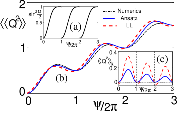
Figure 8: (Color online) (a) Evolution of the extra eigenvalue $\sin^{2}\frac{\alpha_{0}}{2}$ with $\psi$ in (19) . (b) Noise computed from three approaches: Numerics (dash dotted), ansatz (32) (solid) and LL’s result (20) (dashed). (c) $\langle\langle Q^{2}\rangle\rangle_{x}$ (see text) computed for LL’s result and ansatz (32).

To test above idea, as well as to obtain the unknown eigenvalue $\sin^{2}\frac{\alpha_{0}}{2}$, we compute the FCS and the values $\sin^{2}\frac{\alpha_{j}}{2}$ for (30) numerically for different total phase shift $\psi$ in (19). The pulse separation is fixed at $t_{0}/\tau=500$ and the contact transparency is $T=1/2$. With cut-off energy $\xi$ as the only fitting parameter, the ansatz (31) agrees with the numerical result for $\chi(\lambda)$ in the parameter space $\{\psi,\lambda\}$ everywhere with a maximum difference of 3%. This agreement justifies our decomposition of $\chi(\lambda)$ based on the separation of eigenvalues of $n^{out}$. The evolution of $\sin^{2}\frac{\alpha_{0}}{2}$ with $\psi$ is drawn in Fig. 8(a) and echoes that reported for a tunnel junction driven by a sinusoidal voltage as a function of the voltage amplitude.Vanević et al. (2008) As $\psi$ increases, the value $\sin^{2}\frac{\alpha_{0}}{2}$ increases gradually and saturates at $1$.

The noise can be computed using (31) and is

$$\langle\langle Q^{2}\rangle\rangle=2RT[\frac{2}{\pi^{2}}\sin^{2}\frac{\psi_{0}}{2}\ln t_{0}\xi+k+\sin^{2}\frac{\alpha_{0}}{2}].$$ (32)

In Fig. 8(b) we show the noise computed from three approaches: i) exactly computed numerically from (9); ii) using out ansatz (32) and iii) from the expansion used by LL (20). The cut-off energy $\xi$ is used as fitting parameter to give the best agreement with the exact result. The similarity between the noise produced here and the noise generation in Fig. 7(b) for fixed $t_{f}$ can be understood using the mapping between the problem we are considering here of an applied bias voltage and that of a modulate barrier profile discussed in Sec. II.2. In both cases the contribution proportional to the $\log t_{0}\xi$ is suppressed at quantized phase shift $\psi$.

The differences between the two approximate treatments and the exact results are associated with the “large” eigenvalues. We define the quantity $\langle\langle Q^{2}\rangle\rangle_{x}=\langle\langle Q^{2}\rangle\rangle_{nu}-2RTx(\psi)$, with $x(\psi)=\frac{\psi}{2\pi}$ for the expansion (20) and $x(\psi)=k+\sin^{2}\frac{\alpha_{0}}{2}$ for our ansatz (31). $\langle\langle Q^{2}\rangle\rangle_{nu}$ is the exact value of the noise computed numerically. According to (20) as well as (32), $\langle\langle Q^{2}\rangle\rangle_{x}$ is proportional to $\sin^{2}\frac{\psi}{2}$, and, if the cut-off energy $\xi$ is independent of $\psi$, is periodic. It should also vanish at $\psi=0,2\pi,4\pi\ldots$. We show $\langle\langle Q^{2}\rangle\rangle_{x}$ for the two cases respectively in Fig. 8(c). We see that the ansatz (32) works qualitatively correctly while the expansion (20) gives the wrong positions for the minima. However, we find that $\langle\langle Q^{2}\rangle\rangle_{nu}$ is not strictly periodic (the amplitude of the oscillation decreases). We attribute this to the fact that the separation into the two factors $\chi_{1}$ (corresponding to $k$ large values of $\sin^{2}\alpha_{j}$) and $\chi_{2}$ (only small values) is not complete and that the value $\sin^{2}\alpha_{k+1}/2$ can be significant particularly for small $k$.

IV Conclusion

We have discussed the Full Counting Statistics (FCS) of the charge transferred across a quantum point contact. We have illustrated the power of a mapping between the case of a biased barrier with constant transmission and reflection amplitudes and the case of a barrier with time-dependent profile but no bias. With this mapping we have showed that known results for the two cases, which had been previously obtained using different, and generally involved calculations, can be understood using the basis of quantized Lorentzian pulsesIvanov et al. (1997) or Minimal Excitation StatesKeeling et al. (2006) (MES). Examples include the optimal protocol for electron entanglement, Sherkunov et al. (2009) the FCS of a sinusoidally driven barrier, Andreev and Kamenev (2000) and the Fermi Edge Singularity. Nozieres and De Dominicis (1969)

For the purposes both of conceptual understanding and computation, we have argued that the problem is simplest when approached through the eigenvalues of the density matrix of the outgoing states in one of the leads. For the general case, which corresponds to applying both a bias and varying the barrier profile with time, we have developed a numerical scheme for computing exactly the FCS for a device and used this to compute the FCS for a tunnel barrier operated as an electron source. We have also studied how the deviation from an ideal pulse affect the quality of operation of a device with low noise or an entangler. We showed that the noise levels were remarkably insensitive to deviations from quantized Lorentzian pulses associated with the long-time behavior. For deviations away from the quantization of the pulses in the case of a modulation of barrier profile, we found that, as expected, this led to the reappearance of the equilibrium noise contribution, which increases logarithmically with barrier opening time (see Fig. 7).

This work is supported by EPSRC-GB (Contract No. EP/D065135/1).

Appendix A Numerical Diagonalization of (6)

We describe the numerical procedure for diagonalizing $n^{out}$ in (6). We need a discretized finite dimensional expression for $\mathbf{XnX}^{\dagger}$, where $\mathbf{X}$ stands for the transmission and reflection matrices $\mathbf{A}$ and $\mathbf{B}$ in frequency space. $\mathbf{n}$ is an infinite dimensional diagonal matrix with elements $n_{mn}=\delta_{mn}\theta(-m+\epsilon)$, where $\epsilon<\omega_{0}$, to avoid $m=0$ in the $\theta$-function. The matrix $\mathbf{X}$ is blockwise tridiagonal:

$$\mathbf{X}=\left(\begin{array}[]{ccccc}\ddots&\ddots&\ddots&\mbox{}&\mbox{}\\ \mbox{}&\mathbf{X}_{2}&\mathbf{X}_{0}&\mathbf{X}_{1}&\mbox{}\\ \mbox{}&\mbox{}&\ddots&\ddots&\ddots\end{array}\right),$$

where $\mathbf{X}_{0,1,2}$ is square matrix with truncated dimension $M$ (see main text). $\mathbf{X}_{1}$ ($\mathbf{X}_{2}$) is lower (upper) triangular matrix with null diagonal elements.

Exploiting the property $B(t)B^{\ast}(t)+A(t)A^{\ast}(t)=1$, which in frequency space states $\mathbf{B}\mathbf{B}^{\dagger}+\mathbf{A}\mathbf{A}^{\dagger}=\mathbf{I}$ ($\mathbf{I}$ is the infinite dimensional identity matrix), we find the following properties for the finite block sub-matrices with dimension $M$: $\sum_{i=0}^{2}(\mathbf{B}_{i}\mathbf{B}_{i}^{\dagger}+\mathbf{A}_{i}\mathbf{A}_{i}^{\dagger})=\mathbf{I}$, $\mathbf{B}_{2}\mathbf{B}_{0}^{\dagger}+\mathbf{B}_{0}\mathbf{B}_{1}^{\dagger}+\mathbf{A}_{2}\mathbf{A}_{0}^{\dagger}+\mathbf{A}_{0}\mathbf{A}_{1}^{\dagger}=\mathbf{0}$, and $\mathbf{A}_{1}\mathbf{A}_{2}^{\dagger}=\mathbf{B}_{1}\mathbf{B}_{2}^{\dagger}=\mathbf{0}$.

Compute $n^{out}$ in (6) in frequency space and remove the part equivalent to $n^{in}$ at low and high energies, we arrive at a much simplified form of $n^{out}$ suitable for numerical diagonalization

$$\mathbf{n}^{out}=\left(\begin{array}[]{cc}\mathbf{B}_{1}\mathbf{B}_{1}^{\dagger}+\mathbf{A}_{1}\mathbf{A}_{1}^{\dagger}&\mathbf{B}_{1}\mathbf{B}_{0}^{\dagger}+\mathbf{A}_{1}\mathbf{A}_{0}^{\dagger}\\ \mathbf{B}_{0}\mathbf{B}_{1}^{\dagger}+\mathbf{A}_{0}\mathbf{A}_{1}^{\dagger}&\mathbf{I}-\mathbf{B}_{2}\mathbf{B}_{2}^{\dagger}-\mathbf{A}_{2}\mathbf{A}_{2}^{\dagger}\end{array}\right).$$ (33)

The sought-after spectrum, $n_{j}$, is obtained by diagonalizing (33) directly.

Appendix B Riemann-Hilbert solution to the FCS for barrier opening at non-zero temperature

Here we give a brief derivation of the FCS for the pure opening problem (region 2, Sec. II.3) within the Riemann-Hilbert approach at finite temperature. The scattering matrix $S(t)$ in (23) takes the form

$$S(t)=\left(\begin{array}[]{cc}\cos\frac{\phi}{2}&\sin\frac{\phi}{2}\\ -\sin\frac{\phi}{2}&\cos\frac{\phi}{2}\end{array}\right),~{}\mbox{for t}\in[0,t_{f}]$$

and equals the identity otherwise. Following the notation in Ref. Muzykantskii and Adamov, 2003; d’Ambrumenil and Muzykantskii, 2005, we introduce the matrix $R(\lambda)=Se^{i\lambda L}S^{\dagger}e^{-i\lambda L}$, with $L=\begin{pmatrix}1&0\\ 0&0\end{pmatrix}$. The characteristic function $\ln\chi$ reads

$$\ln\chi(\lambda)=\mbox{Tr}[n\ln R]+\mbox{Tr}[\ln(1-n+nR)-n\ln R]$$ (34)

where Tr operates on both time and channel space. $n$ is the fermionic operator at finite temperature $1/\beta$:

$$n(t,t^{\prime})=\frac{i}{2\pi}\frac{\pi/\beta}{\sinh(\pi(t-t^{\prime})/\beta+i0)}.$$

Since there is no average charge transfer, the first term of (34), $\mbox{Tr}[n\ln R]=i\lambda\langle Q\rangle$, is equal to zero. The FCS is given by the second term,

$$\ln\chi(\lambda)=\frac{i}{2\pi}\int_{0}^{\lambda}d\lambda\int dt~{}\mbox{tr}\left[\frac{d\ln Y_{+}}{dt}\frac{d\ln R}{d\lambda}\right],$$

where tr is a trace over channel space only. The Riemann-Hilbert solution $Y(z)$ is a bounded matrix-valued analytic function in the strip $-\beta/2<\mbox{Im}z<\beta/2$ except along the cut $z\in[0,t_{f}]$, where $Y_{-}(t)Y_{+}^{-1}(t)=R(\lambda)$ $Y_{+}(t)\equiv Y(t+i0)$ and $Y_{-}(t)\equiv Y(t-i0)$ (see Ref. Muzykantskii and Adamov, 2003; d’Ambrumenil and Muzykantskii, 2005; Braunecker, 2006). Making the substitution $\sin\frac{\lambda_{\ast}}{2}=\sin\frac{\phi}{2}\sin\frac{\lambda}{2}$, $R(\lambda)$ can be diagonalized in a time-independent basis with eigenvalues $e^{\pm i\lambda_{\ast}}$. Using explicitly the finite temperature solution of the RH problem,Braunecker (2006)

$$Y_{+}(t)=\exp\left(\frac{1}{2\pi i}\int_{0}^{t_{f}}dt^{\prime}\frac{\cosh(\pi t/\beta)}{\cosh(\pi t^{\prime}/\beta)}\frac{\pi\ln R/\beta}{\sinh(\pi(t-t^{\prime})/\beta)}\right)$$

we obtain

$$\ln\chi(\lambda)=-\frac{\lambda_{\ast}^{2}}{2\pi^{2}}\ln\left(\frac{\sinh(\pi t_{f}/\beta)}{\sinh(\pi\xi^{-1}/\beta)}\right),$$

with $\xi$ as a cut-off. Taking the zero temperature limit $\beta\rightarrow\infty$, we arrive at the characteristic function (23) along with definitions (24) and (25).

References

- Levitov and Lesovik (1993) L. Levitov and G. Lesovik, JETP Letters 58, 230 (1993).
- Gustavsson et al. (2006) S. Gustavsson, R. Leturcq, B. Simovič, R. Schleser, T. Ihn, P. Studerus, K. Ensslin, D. C. Driscoll, and A. C. Gossard, Phys. Rev. Lett. 96, 076605 (2006).
- Fujisawa et al. (2006) T. Fujisawa, T. Hayashi, R. Tomita, and Y. Hirayama, Science 312, 1634 (2006).
- Gustavsson et al. (2008) S. Gustavsson, I. Shorubalko, R. Leturcq, S. Schön, and K. Ensslin, Applied Physics Letters 92, 152101 (2008).
- Levitov et al. (1996a) L. Levitov, H. Lee, and G. Lesovik, J. Math. Phys. 37, 4845 (1996a), cond-mat/9607137.
- Ivanov et al. (1997) D. A. Ivanov, H. W. Lee, and L. S. Levitov, Phys. Rev. B 56, 6839 (1997).
- Belzig and Nazarov (2001) W. Belzig and Y. V. Nazarov, Phys. Rev. Lett. 87, 197006 (2001).
- Muzykantskii and Adamov (2003) B. Muzykantskii and Y. Adamov, Phys. Rev. B 68, 155304 (2003).
- d’Ambrumenil and Muzykantskii (2005) N. d’Ambrumenil and B. Muzykantskii, Phys. Rev. B 71, 045326 (2005).
- Keeling et al. (2006) J. Keeling, I. Klich, and L. S. Levitov, Phys. Rev. Lett. 97, 116403 (2006).
- Vanević et al. (2007) M. Vanević, Y. V. Nazarov, and W. Belzig, Phys. Rev. Lett. 99, 076601 (2007).
- Abanov and Ivanov (2008) A. G. Abanov and D. A. Ivanov, Phys. Rev. Lett. 100, 086602 (2008).
- Neder et al. (2007) I. Neder, N. Ofek, Y. Chung, M. Heiblum, D. Mahalu, and V. Umansky, Nature 448, 333 (2007).
- Beenakker et al. (2004) C. W. J. Beenakker, D. P. DiVincenzo, C. Emary, and M. Kindermann, Phys. Rev. Lett. 93, 020501 (2004).
- Beenakker et al. (2005) C. W. J. Beenakker, M. Titov, and B. Trauzettel, Phys. Rev. Lett. 94, 186804 (2005).
- Trauzettel et al. (2006) B. Trauzettel, A. N. Jordan, C. W. J. Beenakker, and M. Buttiker, Phys.Rev. B 73, 235331 (2006).
- Samuelsson et al. (2009) P. Samuelsson, I. Neder, and M. Büttiker, Phys. Rev. Lett. 102, 106804 (2009).
- Andreev and Kamenev (2000) A. Andreev and A. Kamenev, Phys. Rev. Lett. 85, 1294 (2000).
- Samuelsson et al. (2004) P. Samuelsson, E. V. Sukhorukov, and M. Büttiker, Phys. Rev. Lett. 92, 026805 (2004).
- Beenakker (2006) C. W. J. Beenakker, in Proc. Int. School Phys E. Fermi (IOS Press, Amsterdam, 2006).
- Fevè et al. (2007) G. Fevè, A. Mahe, J.-M. Berroir, T. Kontos, B. Placais, D. Glattli, A. Cavanna, B. Etienne, and Y. Jin, Science 316, 1169 (2007).
- Sherkunov et al. (2008) Y. B. Sherkunov, A. Pratap, B. Muzykantskii, and N. d’Ambrumenil, Phys. Rev. Lett. 100, 196601 (2008).
- Sherkunov et al. (2009) Y. Sherkunov, J. Zhang, N. d’Ambrumenil, and B. Muzykantskii, Phys. Rev. B 80, 041313(R) (2009).
- Abanov and Ivanov (2009) A. G. Abanov and D. A. Ivanov, Phys. Rev. B 79, 205315 (2009).
- Gershon et al. (2008) G. Gershon, Y. Bomze, E. V. Sukhorukov, and M. Reznikov, Phys. Rev. Lett. 101, 016803 (2008).
- Klich (2003) I. Klich, Full Counting Statistics: An elementary derivation of Levitov’s formula (Kluwer, 2003).
- Avron et al. (2007) J. E. Avron, S. Bachmann, G. M. Graf, and I. Klich, Communications in Mathematical Physics 280, 807 (2007).
- Lee and Levitov (1993) H. Lee and L. Levitov (1993), cond-mat/9312013.
- Moskalets and Büttiker (2007) M. Moskalets and M. Büttiker, Phys. Rev. B 75, 035315 (2007).
- (30) I. Klich and L. Levitov, quant-ph/0812.0006.
- Levitov et al. (1996b) L. S. Levitov, H. W. Lee, and G. Lesovik, J. Math. Phys. 37, 4845 (1996b).
- Klich and Levitov (2009) I. Klich and L. Levitov, Phys. Rev. Lett. 102, 100502 (2009).
- Mahan (1967) G. Mahan, Phys. Rev. 163, 1612 (1967).
- Nozieres and De Dominicis (1969) P. Nozieres and C. T. De Dominicis, Physical Review 178, 1079 (1969).
- Anderson (1967) P. Anderson, Phys. Rev. Lett. 18 (1967).
- Schönhammer (2007) K. Schönhammer, Phys. Rev. B 75, 205329 (2007).
- (37) K. Schönhammer, cond-mat/0908.1892 (2009).
- Keeling et al. (2008) J. Keeling, A. V. Shytov, and L. S. Levitov, Phys. Rev. Lett. 101, 196404 (2008).
- Blanter and Buttiker (2000) Y. Blanter and M. Buttiker, Physics Reports 336, 2 (2000).
- (40) We have also looked at the case where a Gaussian pulse is used to approximate the delta function as . The result doesn’t show any significant difference.
- Vanević et al. (2008) M. Vanević, Y. V. Nazarov, and W. Belzig, Phys. Rev. B 78, 245308 (2008).
- Braunecker (2006) B. Braunecker, Phys. Rev. B 73, 075122 (2006).