Computing absolute free energies of disordered structures by molecular simulation

Abstract

We present a Monte Carlo simulation technique by which the free energy of disordered systems can be computed directly. It is based on thermodynamic integration. The central idea is to construct an analytically solvable reference system from a configuration which is representative for the state of interest. The method can be applied to lattice models (e.g., the Ising model) as well as off-lattice molecular models. We focus mainly on the more challenging off-lattice case. We propose a Monte Carlo algorithm, by which the thermodynamic integration path can be sampled efficiently. At the examples of the hard sphere liquid and a hard disk solid with a defect we discuss several properties of the approach.

The fundamental equation $S=f(U,V,\{N_{\alpha}\})$, which connects the entropy $S$ with the internal energy $U$, the volume $V$, and the numbers $N_{\alpha}$ of particles of type $\alpha$, contains all information about a system that is accessible within classical thermodynamics. Other thermodynamic potentials such as e.g. the free energy are related to the fundamental equation by Legendre transform, and hence they equally contain this information Jelitto (1989). Therefore there is large interest in computing free energies in many areas of science, i.e., statistical physics, materials science, theoretical chemistry, and biology Chipot and Pohorille (2007).

There are only very few, special cases in which the free energy of a system can be computed directly: Either the accessible phase space volume can be enumerated completely (as e.g. for a lattice gas model on a small lattice), or the problem can be solved analytically in the first place (as e.g. for the ideal gas). In all other cases one must resort to approximations or to computer simulations. Unfortunately, the latter only give access to free energy derivatives and free energy differences. Several advanced techniques have been developed that allow to relate free energies of different state points to each other, and a large body of literature has been written on this topic Chipot and Pohorille (2007); Earl and Deem (2005); Okamoto (2004); Panagiotopoulos (2000); de Pablo et al. (1999); Bruce et al. (2000); Wilding and Bruce (2000). Nevertheless, comparing the free energies of arbitrary systems remains a challenge, and alternative approaches that allow to determine the absolute free energy for each individual system are clearly of interest.

On principle, absolute free energies can be obtained by connecting the system of interest with a reference system of known free energy. In this letter, we propose a general strategy for the construction of analytically solvable reference systems, that can be connected with a wide class of structures via thermodynamic integration.

Thermodynamic integration Frenkel and Smit (2002); Landau and Binder (2005) is a widely applied method to determine free energy differences. The basic idea is the following: Consider a system of $N$ particles with a Hamiltonian $H(\bm{r}^{N},\bm{p}^{N},\varepsilon)$, which explicitly depends on some parameter $\varepsilon$. In order to obtain an expression for the free energy of the system, one uses the relation ${\partial F}/{\partial\varepsilon}=\left\langle{\partial H(\varepsilon)}/{\partial\varepsilon}\right\rangle$, where $\langle\ldots\rangle$ denotes the thermodynamic average. Here and in the following, we set $k_{B}T=1$. In general, $\langle\partial H(\varepsilon)/\partial\varepsilon\rangle$, is directly accessible in a simulation. Thus the expression above can be used to evaluate the free energy difference between two systems at different $\varepsilon$: One samples $\left\langle{\partial H(\varepsilon)}/{\partial\varepsilon}\right\rangle$ for a range of $\varepsilon$ and integrates

$$\Delta F=F(\varepsilon_{1})-F(\varepsilon_{0})=\int_{\varepsilon_{0}}^{\varepsilon_{1}}\>\mathrm{d}\varepsilon^{\prime}\,\bigg{\langle}\frac{\partial H(\varepsilon^{\prime})}{\partial\varepsilon^{\prime}}\bigg{\rangle}_{\varepsilon^{\prime}}\quad.$$ (1)

If the free energy is known for one $\varepsilon_{0}$ (reference system), the method can be used to calculate absolute free energies for a whole range of $\varepsilon$. However, it is crucial that the evolution of $\langle\partial H(\epsilon)/\partial\varepsilon\rangle$ on the integration path is reversible, i.e., no phase transition of first order may be crossed. This limits the choice of suitable integration paths and reference systems. For gases the ideal gas is a useful reference system, for crystals the “Einstein crystal” (a crystal where the particles are bound to sites of a fixed lattice by harmonic springs Einstein (1907); Frenkel and Ladd (1984)). To the best of our knowledge, no general reference system has been introduced so far that can be used for arbitrary dense disordered systems.

Our central idea to remedy this situation is very simple. We propose to take a configuration that is representative for the structure of interest (obtained e.g. within a typical simulation of an equilibrated system) and to construct a reference system by first ’pinning’ this configuration with suitable external fields, and then switching off the internal interactions. In the remainder of this letter, we will show how this idea can be exploited to evaluate absolute free energies in practice.

For the purpose of illustration, we begin by considering the Ising model $H_{0}=-J\sum_{\langle ij\rangle}s_{i}s_{j}$, where $\langle ij\rangle$ denotes neighbouring $i$ and $j$ and $s_{i}=\pm 1$. To evaluate the free energy $F_{0}$ at a given temperature, we simulate the system until it is equilibrated, and then pick one typical configuration $\{s_{i}^{R}\}$ as ’representative’ reference configuration. The reference system is then defined by the Hamiltonian

$$H_{\rm ref}(\varepsilon)=-\varepsilon\sum_{i}s_{i}s_{i}^{R}\quad,$$ (2)

and its free energy can be computed easily, $F_{\rm ref}(\varepsilon)=-N\ln\left(2\cosh\left(\varepsilon\right)\right)$. To establish the connection with the original system, we procede in two steps: First we define an intermediate model $H^{\prime}(\varepsilon)=H_{0}+H_{\rm ref}(\varepsilon)$, which reduces to $H_{0}$ at $\varepsilon=0$. The free energy difference $\Delta F_{1}(\varepsilon)=F_{0}-F^{\prime}(\varepsilon)$ between the original system and the intermediate system can be calculated for arbitrary $\varepsilon$ by thermodynamic integration, using $\langle\partial H^{\prime}/\partial\varepsilon\rangle=-\langle\sum_{i}s_{i}s_{i}^{R}\rangle$. We choose $\varepsilon$ large enough that the spins in the system $H^{\prime}(\varepsilon)$ hardly fluctuate about the reference value. The second step is to connect the intermediate system to the reference system. The free energy difference between the two systems at the same value of $\varepsilon$, $\Delta F_{2}(\varepsilon)=F^{\prime}(\varepsilon)-F_{\rm ref}(\varepsilon)$, is evaluated by carrying out a simulation with additional Monte Carlo (MC) moves that switch on and off the interaction $J$ according to a Metropolis criterion. We obtain $\Delta F_{2}(\varepsilon)=-\ln(P_{\rm on}/P_{\rm off})$, where $P_{\rm on,off}$ is the fraction of configurations with interactions switched on (rsp. off) in the simulation. Combining everything, we can finally calculate the absolute free energy of the target system $H_{0}$, $F_{0}=F_{\rm ref}(\varepsilon)+\Delta F_{1}(\varepsilon)+\Delta F_{2}(\varepsilon)$.

Now we transfer this idea to off-lattice particle models. For clarity, we only discuss monatomic liquids and solids in the $NVT$ ensemble in the following. Our method can easily be generalized to molecular systems, and, as we shall demonstrate below, to constant pressure simulations. Furthermore, we disregard the kinetic contribution to the free energy, which can be evaluated trivially Hansen and McDonald (2000).

Let configurations be characterized by a set of coordinates $\{\bm{r}_{i}\}$ and the configurational energy be given by a Hamiltonian $H_{0}=U(\{\bm{r}_{i}\})$. To calculate the free energy of a given, arbitrary equilibrium structure, we choose a ’representative’ configuration $\{\bm{r}^{R}_{i}\}$, obtained, e.g., from a simulation of an equilibrated system, and construct a reference system by imposing local potentials

$$H_{\rm ref}(\varepsilon)=\varepsilon\sum_{i}\Phi\left(\frac{|\bm{r}_{i}-\bm{r}^{R}_{i}|}{r_{\rm cutoff}}\right)\quad,$$ (3)

that pin the particles’ positions $\bm{r}_{i}$ to the reference positions $\bm{r}^{R}_{i}$. Here $\Phi$ defines attractive potential-wells centered at each position $\bm{r}^{R}_{i}$, with $\Phi(x)<0$ for $x<1$ and $\Phi\equiv 0$ elsewhere. Note that particle $i$ can only be trapped by well $i$ and not by the other wells. To make the particles indistinguishable, as they should be, we allow them to swap identities (i.e., labels $i,j$) at regular intervals during the simulations. We will show below that such identity swaps are also necessary to equilibrate the system efficiently.

The (configurational) reference free energy is given by

$$\frac{F_{\rm ref}(\varepsilon)}{N}=\ln\left(\frac{N}{V}\right)-\ln\left(1+\frac{V_{0}}{V}g_{\Phi}(\varepsilon)\right)\quad,$$ (4)

where $V_{0}$ is the volume of the sphere of radius $r_{\rm cutoff}$ and $g_{\Phi}(\varepsilon):={\rm d}\int_{0}^{1}dx\;x^{{\rm d}-1}\left(e^{-\varepsilon\Phi(x)}-1\right)$ for a ${\rm d}$-dimensional problem. In our simulations, we mostly used a linear well potential, $\Phi^{\rm linear}(x)=x-1$. In this case one has $g_{\Phi}(\varepsilon)={\rm d}/{\varepsilon^{\rm d}}\left(e^{\varepsilon}\>-\sum_{k=0}^{\rm d}{\varepsilon^{k}}/{k!}\right)$. As before, we also define an intermediate model $H^{\prime}(\varepsilon)=H_{0}+H_{\rm ref}(\varepsilon)$, and evaluate the free energy difference between the reference system and the intermediate system at high $\varepsilon$ with a MC simulation where the interaction $H_{0}$ is switched on and off (if necessary, in several steps). The free energy difference between the target system and the intermediate system is computed by sampling $\partial F^{\prime}/\partial\epsilon=\langle\sum_{i}\Phi(|\bm{r}_{i}-\bm{r}^{R}_{i}|/r_{\rm cutoff})\rangle$ and performing a thermodynamic integration. The remaining challenge is to devise an algorithm for sampling the intermediate model efficiently for arbitrary $\varepsilon$.

Before describing such an algorithm, we briefly comment on the relation between our method and the Einstein crystal method to determine free energies of solids Frenkel and Ladd (1984). In the Einstein crystal method, the particles are not swapped, and the reference system is a regular lattice of harmonic wells with infinite cutoff radius. This works well as long as the particles in the target system stay close to their respective well positions. In a liquid, where their mean-square displacement diverges, $\langle\sum_{i}\Phi(|\bm{r}_{i}-\bm{r}^{R}_{i}|/r_{\rm cutoff})\rangle$ diverges as well for small $\varepsilon$ and can no longer be sampled. Therefore the introduction of a finite cutoff is crucial. We note that our method can also be used to evaluate free energies of crystals.

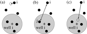
Figure 1: Sketch of moves in our Monte Carlo algorithm. (a) Simple particle displacements. (Could be replaced e.g., by short Molecular Dynamics runs.) (b) Smart particle swaps. (c) Smart particle relocations. See text for explanation

Setting a finite range for the reference potential, however, introduces a different problem: The particles need to find their respective wells of attraction. We therefore introduce two MC moves that help particles $i$ explore their well $i$ (Fig. 1). One move (Fig. 1 b) swaps particles in a smart way. It works as follows:

$\bullet$ Pick a random particle $i$ and find the set of particles $\{n_{i}\}$ that are within the attraction range of well $i$. $\bullet$ If particle $i\notin\{n_{i}\}$: pick a particle $j$ from $\{n_{i}\}$, and swap $i$ and $j$ with the probability $\min\{1,\frac{n_{i}}{N}e^{-\Delta H^{\prime}}\}.$ $\bullet$ Otherwise: pick a particle $j$ from all particles - if $j\notin\{n_{i}\}$: swap with probability $\min\{1,\frac{N}{n_{i}}e^{-\Delta H^{\prime}}\}$. - if $j\in\{n_{i}\}$: swap with probability $\min\{1,e^{-\Delta H^{\prime}}\}.$ Here $\Delta H^{\prime}$ is the difference of the energies (according to the intermediate model) of the old and new configuration. This algorithm promotes particle swaps that bring particles close to their respective well and nevertheless satisfies detailed balance.

The other move (Fig. 1 c) relocates particles $i$ with a bias towards the neighborhood of their well $i$:

$\bullet$ Pick a random particle $i$ (with position $\bm{r}_{i}$). $\bullet$ Choose a new position $\bm{r}^{\prime}_{i}$ from a given (biased) distribution $P_{i}(\bm{r^{\prime}}_{i})=\exp(-W(|\bm{r^{\prime}}_{i}-\bm{r}_{i}^{R}|))$. $\bullet$ Relocate the particle from $\bm{r}$ to $\bm{r}^{\prime}_{i}$ with probability $\min\{1,P(\bm{r}_{i})/P(\bm{r}^{\prime}_{i})\>e^{-\Delta H^{\prime}}\}$. Obvious choices for $W(r)$ which we have tested are $W(r)=\varepsilon\Phi(r/r_{\rm cutoff})$, or $W(r)={\rm const.}$ for $r<r_{\rm cutoff}$. At high $\varepsilon$, the relocation move helps to overcome trapped situations where most particles are bound to a well, and a few cannot escape from a local cage. To illustrate the effect of the different moves, Fig. 2 shows the evolution of the observable $\langle\Phi_{i}\rangle$, averaged over all particles $i$, in a two dimensional system of hard disks, after $\varepsilon$ had been raised from zero to a high value. In a MC simulation that includes only random particle displacements, the system is far from equilibration after one million MC sweeps (a). The smart swap moves speed up equilibration considerably, but the system gets trapped in a configuration where one particle cannot enter its well (b). This problem is solved by including smart relocation moves (c).

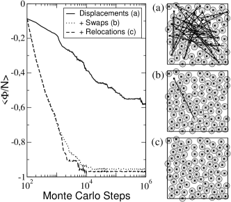
Figure 2: Illustration of the effect of the moves of Fig. 1 on the equilibration of a system of 80 hard disks (diameter $D$) at a density $\rho=0.8/D^{2}$, after switching on linear well potentials with strength $\varepsilon=50$ ($r_{\rm cutoff}=2D$). Swap moves and relocation moves (one per bead) were attempted one per 100 MC sweeps. Left: Evolution of $\langle\Phi\rangle$ in simulations that include different moves as indicated. Right: Corresponding final configurations. Circles indicate particle positions, crosses give well positions. Particles and their respective wells are connected by straight lines.

Table 1: Results for the free energy of hard spheres. ${F/N}_{\rm CS}$ is the value according to the Carnahan-Starling equation of state Carnahan and Starling (1969). a) linear potential $\Phi$, liquid reference state. b) linear $\Phi$, hcp reference state. c) harmonic $\Phi$, liquid reference state.

$N/V$	$F/N$	$(F/N)_{\rm CS}$
$0.25$	$0.62(0)$	$0.625$
$0.5^{a)}$	$1.54(1)$	$1.544$
$0.5^{b)}$	$1.54(0)$	$1.544$
$0.5^{c)}$	$1.54(9)$	$1.544$
$0.75$	$3.00(9)$	$3.005$

We will now demonstrate the power of our approach at a few examples. They are not meant to be self-sufficient scientific studies – the simulations were carried out on simple workstations with poorly optimized test programs in relatively short time (less than a week). We are aware that a careful analysis of the finite-size effects should be done in all cases. Here we only intend to illustrate some properties of the algorithm.

We have studied hard spheres in two (2d) and three dimensions (3d). For the remainder of this letter we use the particle diameter $D$ as unit of length. Table 1 shows results for the free energy of a 3d liquid of hard spheres. The simulations were performed on a system of $N=256$ particles, using 50 values of $\varepsilon$ and $6\cdot 10^{5}$ MC sweeps for each value at $N/V=0.25$ and $N/V=0.5$, and 200 values of $\varepsilon$ times 1 Mio. MC sweeps at $N/V=0.75$. The results agree with the values obtained by integration of the Carnahan-Starling equation of state Carnahan and Starling (1969) within the error bars. For $N/V=0.5$ we compared the cases a) linear potential $\Phi$ and liquid reference state, b) linear $\Phi$ and crystalline reference state, and c) harmonic $\Phi$ and liquid reference state. Within the error-bars these variations produce the same result. However, for more accurate calculations the linear potential seems to be most useful, because the particles get trapped most efficiently. In case b) we did not see a hysteresis on increasing/decreasing $\varepsilon$. Apparently, the trapping of particles in a crystalline array of wells is not associated with a phase transition at this density. This will presumably be different closer to liquid/solid coexistence. Nevertheless we can conclude that our method is quite robust and may work even if the reference configuration is not ’ideal’, i.e., not representative of the target structure.

Next we show an example for the application of the method to dense disordered systems, where the dynamics is driven by cooperative processes. We studied hard disks in 2d up to densities where the equilibrium phase is a solid, and enforced a vacancy defect by taking one particle out of an otherwise ordered configuration. These simulations were carried out at constant pressure $P$ in a rectangular simulation box of varying area, but fixed side ratio $1:\sqrt{3/4}$, to accomodate a triangular lattice. The defect is then stable, but highly mobile.

We compare three different structures (Fig. 3): An ordered solid (a), an ordered solid with a vacancy (b), and a metastable disordered jammed phase (c), which was obtained by compressing the system from the fluid phase. Free energy calculations were carried out at $P=10$ for these three cases, and additionally at $P=6$, in the fluid regime. To calculate the free energy in the enthalpic ensemble, we use a reference system that is defined in terms of scalable coordinates (i.e., the positions of the well centers are rescaled along with the particle coordinates if the volume of the system changes), and pin the volume of the system by an additional term $\varepsilon(V-V_{\rm ref})^{2}$ in the reference Hamiltonian. The thermodynamic integration was carried out for $\varepsilon=0\ldots 40$ using 66 values of $\varepsilon$, and 10 Mio. MC sweeps for each $\varepsilon$. The resulting free enthalpies $G$ can be related to the chemical potential $\mu$ by virtue of the thermodynamic relation $G=\mu N$.

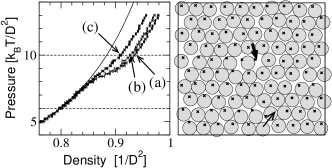
Figure 3: Characterization of the dense two-dimensional systems discussed in the text. Left: Pressure vs. density as obtained from constant pressure simulations at $\varepsilon=0$. (a) $N=100$ particles, expanded from an ordered solid phase, (b) $N=99$ particles, expanded from an ordered solid phase with one vacancy, (c) $N=100$ particles (diameter $D$), compressed from the fluid phase. The solid line shows the theoretical estimate $P=\hat{\rho}/(1-\frac{\pi}{4}\hat{\rho})^{2}$ with $\hat{\rho}=(N+1)/\langle V\rangle$. Right: A configuration with one vacancy at the beginning (crosses) and the end (circles) of a MC run. The thin and thick arrows mark the position of the defect at the beginning and the end.

To set the frame, we show in Fig. 3 a) the pressure-density curves for the cases a),b), and c). In the fluid regime ($\rho\leq 0.8$), they can be fitted nicely with the theoretical estimate Helfand et al. (1960) $P=\hat{\rho}/(1-\frac{\pi}{4}\hat{\rho})^{2}$ with $\hat{\rho}=(N+1)/\langle V\rangle$. Fig. 3 b) illustrates the mobility of the defect at pressure $P=10$. It should be noted that in the solid regime, the center of mass motion of the complete system is not sampled well, because individual particles stay close to their lattice sites. A similar problem is encountered in the Einstein crystal method and has lead to the development of the ‘Einstein molecule’ Vega and Noya (2007), where the reference crystal is defined in terms of relative coordinates. This idea can easily be transfered to our approach. Here, we ignore the center-of-mass correction, because it is smaller than our statistical error.

At $P=6$, the free energy calculation yields the free enthalpy per particle $\mu=8.997(2)$, which is reasonably close to the theoretical estimate $\mu=9.047$ obtained by integrating the theoretical equation of state. At $P=10$, we found $\mu_{\rm solid}=13.617(2)$ in the solid state, and $\mu_{\rm jam}=13.675(2)$ in the jammed state, which establishes that the solid is indeed the stable phase. For the system with one defect, we obtained the total enthalpy $G_{\rm defect}=1361.7(2)$. This result can be used to estimate the core free energy of the vacancy $\mu_{c}=G_{\rm defect}-\mu_{\rm solid}N+\ln(N)=7.1(3)$, which corresponds to a relative vacancy frequency of roughly $10^{-3}$. (For comparison, the frequency of vacancies at liquid/solid coexistence in 3d is roughly $10^{-4}$ Pronk and Frenkel (2001).) Probably $\mu_{c}$ is largely overestimated due to finite size effects, hence the value given above is at best an upper bound. More detailed studies shall be carried out in the future. Here, the example mainly serves to illustrate the use of our approach in situations where free energies are difficult to access with other methods.

In summary, we have introduced a general method to compute absolute free energies for a wide range of structures. We have illustrated the method for monatomic simple systems, but we believe that it can be applied equally well to molecular fluids and mixtures. We anticipate that our method will be useful to calculate free energies of systems that are not directly connected with the ideal gas, such as liquid crystal phases, membranes, or proteins in solution. Also defects in solids seem to be a promising field of application. From a fundamental point of view, it should be interesting to study how well the method can be applied to glassy systems, which have not just one, but a whole set of ’representative’ configurations, one for each local minimum in the rugged free energy landscape.