FUSE Measurements of Far-Ultraviolet Extinction. III. The Dependence on R(V)
and Discrete Feature Limits from 75 Galactic Sightlines

Abstract

We present a sample of 75 extinction curves derived from FUSE far-ultraviolet spectra supplemented by existing IUE spectra. The extinction curves were created using the standard pair method based on a new set of dereddened FUSE+IUE comparison stars. Molecular hydrogen absorption features were removed using individualized $H_{2}$ models for each sightline. The general shape of the FUSE extinction ($8.4~{}\micron^{-1}<\lambda^{-1}<11~{}\micron^{-1}$) was found to be broadly consistent with extrapolations from the IUE extinction ($3.3~{}\micron^{-1}<\lambda^{-1}<8.6~{}\micron^{-1}$) curve. Significant differences were seen in the strength of the far-UV rise and the width of the 2175 Å bump. All the FUSE+IUE extinction curves had positive far-UV slopes giving no indication that the far-UV rise was turning over at the shortest wavelengths. The dependence of $A(\lambda)/A(V)$ versus $R(V)^{-1}$ in the far-UV using the sightlines in our sample was found to be stronger than tentatively indicated by previous work. We present an updated $R(V)$ dependent relationship for the full UV wavelength range ($3.3~{}\micron^{-1}\leq\lambda^{-1}\leq 11~{}\micron^{-1}$). Finally, we searched for discrete absorption features in the far-ultraviolet. We found a 3$\sigma$ upper limit of $\sim$$0.12A(V)$ on features with a resolution of 250 ($\sim$4 Å width) and 3$\sigma$ upper limits of $\sim$$0.15A(V)$ for $\lambda^{-1}<9.6$ µm^-1 and $\sim$$0.68A(V)$ for $\lambda^{-1}>9.6$ µm^-1 on features with a resolution of $10^{4}$ ($\sim$0.1 Å width).

1. Introduction

Extinction curves are one of the cornerstones of our understanding of dust in interstellar space. Extinction curves probe the sum of the absorption and scattering of dust and their determination is observationally straightforward. Most extinction curves are measured using the standard pair method (Stecher, 1965; Massa et al., 1983) where the measurements of a reddened star are ratioed to those of an unreddened star of the same spectral type. The importance of measuring extinction curves over the widest wavelength range possible is attested to by their use as a fundamental constraint in models of dust grains (Weingartner & Draine, 2001; Clayton et al., 2003b; Zubko et al., 2004). Measuring extinction curves is also important for purely empirical reasons in order to allow for the proper accounting for the effects of interstellar dust in the study of astrophysical objects.

Structure in interstellar extinction curves gives direct evidence of the dust grain compositions. In the ultraviolet, the one very obvious discrete feature is the 2175 Å extinction bump (Stecher, 1965, 1969). The 2175 Å bump has been observed to have nearly constant central wavelength, a width varying from 280–660 Å (Fitzpatrick & Massa, 1986; Valencic et al., 2004; Fitzpatrick & Massa, 2007), and has been attributed to small graphite grains (Stecher & Donn, 1965; Draine & Malhotra, 1993). There have been no other discrete features found in the ultraviolet with fairly sensitive limits placed from searches (Clayton et al., 2003a) for counterparts of the optical/near-infrared Diffuse Interstellar Bands (DIBs, Merrill, 1934; Herbig, 1995). The other main structure seen in the ultraviolet extinction curve is the far-ultraviolet (far-UV) rise. This rise is characterized by a constant shape between 1700 and 1175 Å (Fitzpatrick & Massa, 1988) and has been modeled as the wing of a feature like the 2175 Å bump, but centered at 715 Å (Joblin et al., 1992; Li & Draine, 2001).

The structure in the ultraviolet between 1175 and 3300 Å has been well studied using spectra taken with the International Ultraviolet Explorer (IUE) (Fitzpatrick & Massa, 1990; Valencic et al., 2004) and the Space Telescope Spectrograph on the Hubble Space Telescope (Clayton et al., 2003a). The structure in this wavelength range is well approximated by the Fitzpatrick & Massa (1990) (hereafter FM90) parameterization with the curve being the combination of a linear term, a Drude profile, and a cubic describing the far-UV rise. In addition, the average behavior of ultraviolet extinction was found by Cardelli et al. (1989) (hereafter CCM89) to correlate with $R(V)=A(V)/E(B-V)$ (a rough measure of the average dust grain size). More recently, Fitzpatrick & Massa (2007) have proposed a revised parameterization that includes an additional parameter and simplifies the far-UV curvature term to just a quadratic.

Table 1Comparison Stars

name	SpType	V	A(V)	R(V)	C1	C2	C3	C4	xo	$\gamma$
V, main sequence
HD091824	O6V	8.14	$0.60\pm 0.06$	$3.10\pm 0.31$	$-0.81\pm 0.41$	$0.90\pm 0.22$	$3.69\pm 1.11$	$0.43\pm 0.06$	$4.62\pm 0.09$	$1.00\pm 0.10$
HD093028	O8V	8.37	$0.80\pm 0.12$	$3.20\pm 0.48$	$0.38\pm 0.19$	$0.61\pm 0.15$	$2.07\pm 0.41$	$0.29\pm 0.06$	$4.62\pm 0.18$	$0.87\pm 0.09$
HD097471	B0V	9.30	$0.90\pm 0.09$	$3.10\pm 0.31$	$-0.93\pm 0.47$	$0.88\pm 0.18$	$1.83\pm 0.55$	$0.28\pm 0.06$	$4.62\pm 0.09$	$0.85\pm 0.09$
BD+52$\arcdeg$3210	B1V	10.69	$0.85\pm 0.09$	$3.50\pm 0.35$	$-1.67\pm 0.42$	$0.99\pm 0.15$	$3.43\pm 0.69$	$0.25\pm 0.06$	$4.60\pm 0.09$	$0.91\pm 0.09$
BD+32$\arcdeg$270	B2V	10.29	$0.10\pm 0.04$	$3.10\pm 1.24$	$-0.24\pm 0.12$	$0.74\pm 0.37$	$2.00\pm 1.00$	$0.82\pm 0.41$	$4.59\pm 0.46$	$1.00\pm 0.20$
HD051013	B3V	8.81	$0.10\pm 0.04$	$3.10\pm 1.55$	$-0.24\pm 0.12$	$0.74\pm 0.37$	$2.00\pm 1.00$	$0.42\pm 0.21$	$4.59\pm 0.46$	$1.00\pm 0.20$
HD037332	B4V	7.62	$0.10\pm 0.02$	$3.10\pm 0.60$	$-0.24\pm 0.12$	$0.94\pm 0.47$	$3.56\pm 1.78$	$2.00\pm 0.50$	$4.59\pm 0.46$	$1.00\pm 0.20$
HD037525	B5V	8.08	$0.18\pm 0.09$	$3.10\pm 1.24$	$-0.24\pm 0.12$	$0.74\pm 0.37$	$3.56\pm 1.78$	$0.52\pm 0.26$	$4.59\pm 0.18$	$1.00\pm 0.20$
III, giant
HD116852	O9III	8.47	$0.63\pm 0.06$	$3.01\pm 0.60$	$-0.65\pm 0.33$	$0.70\pm 0.10$	$1.41\pm 0.28$	$0.28\pm 0.07$	$4.56\pm 0.18$	$0.72\pm 0.07$
HD104705	B0III	7.76	$1.06\pm 0.11$	$3.31\pm 0.33$	$0.27\pm 0.13$	$0.49\pm 0.10$	$2.01\pm 0.40$	$0.30\pm 0.03$	$4.56\pm 0.09$	$0.82\pm 0.08$
HD172140	B0.5III	9.94	$0.56\pm 0.11$	$2.34\pm 0.47$	$-0.37\pm 0.18$	$0.61\pm 0.15$	$2.58\pm 0.52$	$0.37\pm 0.06$	$4.59\pm 0.09$	$0.89\pm 0.09$
HD114444	B2III	10.31	$0.51\pm 0.10$	$2.65\pm 0.53$	$-0.65\pm 0.32$	$0.40\pm 0.10$	$2.56\pm 0.51$	$0.31\pm 0.08$	$4.61\pm 0.09$	$0.82\pm 0.08$
HD235874	B3III	9.64	$0.58\pm 0.06$	$2.93\pm 0.29$	$-2.63\pm 0.66$	$1.11\pm 0.11$	$3.26\pm 0.65$	$0.26\pm 0.06$	$4.68\pm 0.09$	$0.97\pm 0.10$
I, supergiant
HD210809	O9Ib	7.54	$0.98\pm 0.05$	$3.10\pm 0.31$	$-1.23\pm 0.31$	$0.98\pm 0.05$	$2.58\pm 0.26$	$0.45\pm 0.02$	$4.60\pm 0.09$	$1.00\pm 0.10$
HD091983	O9.5Ib	8.58	$1.10\pm 0.11$	$3.10\pm 0.23$	$0.35\pm 0.17$	$0.61\pm 0.09$	$2.50\pm 0.50$	$0.40\pm 0.04$	$4.61\pm 0.09$	$0.98\pm 0.10$
HD094493	B0.5Iab	7.27	$0.70\pm 0.04$	$3.30\pm 0.33$	$-1.02\pm 0.51$	$0.95\pm 0.19$	$3.14\pm 0.63$	$0.56\pm 0.08$	$4.60\pm 0.09$	$0.93\pm 0.09$
HD100276	B1Ib	7.22	$0.83\pm 0.08$	$3.50\pm 0.35$	$-1.48\pm 0.37$	$0.92\pm 0.09$	$3.30\pm 0.66$	$0.26\pm 0.06$	$4.59\pm 0.09$	$0.95\pm 0.10$
HD075309	B2Ib	7.85	$0.64\pm 0.06$	$3.53\pm 0.71$	$0.39\pm 0.20$	$0.53\pm 0.13$	$2.59\pm 0.52$	$0.30\pm 0.08$	$4.60\pm 0.09$	$0.76\pm 0.08$

The dust extinction in the far-UV region between 912 and 1190 Å has only been studied for a handful of Milky Way sightlines (see Sofia et al., 2005, for a review). Our understanding of the far-UV extinction and the nature of the dust materials responsible for it is, necessarily, tentative. The many spectra of hot stars taken with the Far-Ultraviolet Spectroscopic Explorer (FUSE, Moos et al., 2000) allow for an extensive study of the extinction curve in the far-UV region and motivate this analysis. The aim is to refine our understanding of the far-UV extinction using a statistically significant sample of FUSE extinction curves. Specifically, we will investigate how well the FM90, CCM89, and Fitzpatrick & Massa (2007) parameterizations extrapolate to the far-UV and refine them if necessary. Also, we will see if the far-UV region contains any significant structure in addition to the well-known far-UV rise.

This study is the third paper in a series of papers investigating FUSE far-UV extinction curves. The first paper in this series (Sofia et al., 2005) presented a preliminary study of far-UV extinction curves along nine Milky Way sightlines. The second paper in this series (Cartledge et al., 2005) presented a study of nine far-UV extinction curves in the Magellanic Clouds. This third paper presents far-UV extinction curves for 75 sightlines and benefits from a more mature FUSE calibration, a better understanding of correcting for the $H_{2}$ absorption, and a more complete set of FUSE comparison stars. The fourth paper in this series Cartledge et al. (2009) will study the correlations between the gas properties (e.g., $H_{2}$, & H I) and dust extinction.

2. Data

The sample of stars for this paper was determined by searching the FUSE archive for stars from the Valencic et al. (2004) (hereafter VGC04) sample of IUE extinction curves that had good quality FUSE spectra. IUE extinction curves are required because the large scale extinction structure in the FUSE wavelength range (far-UV rise) starts in the IUE spectral range around 1700 Å (Fitzpatrick & Massa, 1988). As a side benefit, the existence of IUE extinction curves for all the sightlines studied in this paper ensures that these sightlines are suitable for extinction curve determinations. The final sample for this paper includes 75 sightlines.

The FUSE observations (912 – 1190 Å) were extracted from the archive and reduced using CalFUSE v3.0. The observations used for each star are given in Cartledge et al. (2009). The next step was to generate corrections for the copious $H_{2}$ absorption seen throughout the FUSE spectral region. This was done by determining the physical parameters of the $H_{2}$ absorbing gas and generating a model spectrum of the $H_{2}$ absorption. The details of the $H_{2}$ and H I modeling are given in Cartledge et al. (2009). When correcting a FUSE spectrum for $H_{2}$ and H I absorption, any point which is absorbed by more than 70% was excluded from use in generating an extinction curve, to minimize the effects of the uncertainties in the $H_{2}$ and H I corrections on the resulting extinction curves. The residual effects of the $H_{2}$ and H I absorption on the final extinction curves are discussed in §3.4.

The complimentary IUE spectra (1150 – 3225 Å) were taken from the IUE archive following VCG04. Optical and near-infrared photometry was accumulated from the literature also following VCG04. The spectral overlap between the IUE and FUSE observations was used to derive a multiplicative correction to the FUSE spectra to put them on the same flux scale as the IUE spectra. The corrections are generally small with maximum corrections up to 25%. Finally, the FUSE and IUE spectra were rebinned to a common resolution of 250 which is sufficient for most extinction curve work.

2.1. New Comparison Stars

Calculating an extinction curve for the sightline towards a reddened star requires an unreddened comparison star of the same spectral type. For IUE observations, there exists a good set of bright, lightly reddened comparison stars which have been carefully dereddened (Cardelli et al., 1992). Ideally, FUSE observations of these same IUE comparison stars would be used to extend their spectra to far-UV wavelengths. Unfortunately, many of the IUE comparison stars are too bright to be observable with FUSE. A new set of fainter comparison stars that are observable with FUSE is required.

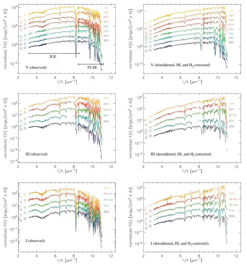
Figure 1.— The FUSE and IUE spectra of the comparison stars are plotted. All the spectra are plotted at a common spectral resolution of 250. The plots on the left give the observed spectra and the same spectra which have been dereddened and corrected for H I and H₂ absorption are on the right. The spectra are normalized to one between 4 and 5 µm^-1 and offset from each other by 0.5 in log space.

We have generated the FUSE set of comparison stars by picking the least reddened star of each spectral type that has both FUSE and IUE observations. The new comparison star sample is listed in Table 1 along with the parameters used to deredden their IUE and FUSE spectra. The $H_{2}$ and H I model parameters used to remove the affects of $H_{2}$ absorption are given by (Cartledge et al., 2009). Given the FUSE brightness limit, these stars are necessarily more distant and reddened than the IUE comparison star sample. We have carefully dereddened these new comparison stars following the methods of Cardelli et al. (1992). The dereddening was done starting with $E(B-V)$, $A(V)$, and Fitzpatrick & Massa (1990) parameters taken from VCG04. Thus, these new comparison stars are directly bootstrapped off of the existing IUE comparison stars. The use of FM parameters determined in the IUE spectral range to deredden FUSE spectra is supported by earlier work on FUSE extinction curves showing that the extrapolation of the FM fits to the FUSE wavelength range is reasonable (Sofia et al., 2005). We have checked that this extrapolation is not affecting our results in §3.3. As was done by Cardelli et al. (1992), the dereddening parameters were then manually tweaked to produce dereddened spectra that lacked obvious dust extinction and had a smooth progression between spectral types. This is illustrated in Fig. 1 where the observed and dereddened spectra for each class of standards (main sequence, giants, and supergiants) are shown. The uncertainties on the dereddening parameters was estimated by changing each parameter until it was clearly incorrect. The resulting uncertainties are given in Table 1 and are assumed to be one sigma uncertainties to be conservative.

An alternative to using observed comparison stars is to use stellar atmosphere models. This is an approach that has been explored by Fitzpatrick & Massa (1999, 2005) and found to produce similar results to using observed comparison stars. The strength of using model atmospheres is that it removes the need to deredden observed spectra and should provide closer spectral matches. The weakness is that it relies on the accuracy of the stellar atmosphere models and the absolute calibration of the spectra. Observed comparison stars only rely on the relative calibration of the spectra and, by definition, include the same physics as the reddened stars. The use of observed comparison stars does inject some additional uncertainty due to the lack of “perfect” matches to the reddened star spectral types. In the end, using observed or model comparison stars represent complimentary approaches, each with strengths and weaknesses. The fact that they produce similar results provides strong evidence that the resulting extinction curves derived from either method are correct.

2.2. Extinction Curve Calculation

The extinction curves were calculated using the standard pair method (Stecher, 1965; Massa et al., 1983). Basically, the ratio of the fluxes of the reddened and comparison stars (both with the same spectral type) gives a direct measurement of the dust extinction towards the reddened star. Ideally, the distances to the reddened and comparison stars would be known to high accuracy, allowing for an absolute measurement of the dust extinction. Unfortunately, the distances to the hot, early-type stars used for ultraviolet dust extinction curve measurements are rarely, if ever, known to high enough accuracy. It is possible then to make a differential measurement of the difference between the colors of reddened and comparison stars. The basic measurement is

$$E(\lambda-V)=m(\lambda-V)_{r}-m(\lambda-V)_{c}$$ (1)

where $r$ and $c$ subscripts refer to the reddened and comparison stars, respectively. This measurement is the unnormalized extinction curve. The use of colors w.r.t. the V band removes the unknown or uncertain distance to each of the stars from the measurement. In order to make comparisons between extinction curves measured along different sightlines, the curve needs to be normalized to a measurement of the total column of dust along the sightline. The most often used normalization is to divide $E(\lambda-V)$ by $E(B-V)$. Yet a more direct measure of the dust properties is $A(\lambda)/A(V)$.

There are two avenues to determining $A(\lambda)/A(V)$ from the basic $E(\lambda-V)$ measurement. The usual method is to determine the conversion factor $R(V)$ [$=A(V)/E(B-V)$] by extrapolating the $E(\lambda-V)/E(B-V)$ curve at JHK wavelengths to infinite wavelength using an assumed form of the $A(\lambda)/A(V)$ curve at wavelengths $>1$ µm. The conversion is then

$$\frac{A(\lambda)}{A(V)}=\frac{1}{R(V)}\left[\frac{E(\lambda-V)}{E(B-V)}\right]+1$$ (2)

A more direct way is to extrapolate the $E(\lambda-V)$ curve to infinite wavelength using the same assumptions [JHK wavelengths and an assumed $A(\lambda)/A(V)$ curve] to determine $A(V)$. The conversion is then

$$\frac{A(\lambda)}{A(V)}=\frac{E(\lambda-V)}{A(V)}+1.$$ (3)

Functionally, both methods of determining $A(\lambda)/A(V)$ are equivalent.

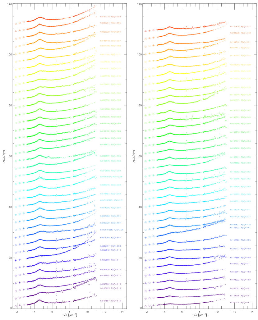
Figure 2.— The extinction curves are plotted for the entire sample along with the FM90 fit to each curve. The curves are plotted sorted by measured $R(V)$ values and offset by a constant value from each other. The reddened star name and measured $R(V)$ value is given to the right of each curve.

Table 2Extinction Curve Details

name	SpType	comparison	V	A(V)	E(B-V)	R(V)
BD+35$\arcdeg$4258	B0.5V	HD097471	9.41	$0.95\pm 0.04\pm 0.03$	$0.31\pm 0.053\pm 0.037$	$3.06\pm 0.380\pm 0.011$
BD+53$\arcdeg$820	B0IV	HD104705	9.95	$1.20\pm 0.04\pm 0.03$	$0.40\pm 0.047\pm 0.035$	$3.01\pm 0.249\pm 0.012$
BD+56$\arcdeg$524	B1V	BD+52$\arcdeg$3210	9.75	$1.80\pm 0.04\pm 0.02$	$0.60\pm 0.044\pm 0.023$	$2.98\pm 0.191\pm 0.009$
HD001383	B1II	HD100276	7.63	$1.36\pm 0.04\pm 0.02$	$0.45\pm 0.035\pm 0.029$	$3.04\pm 0.151\pm 0.009$
HD013268	O8V	HD093028	8.18	$1.35\pm 0.04\pm 0.03$	$0.44\pm 0.052\pm 0.042$	$3.07\pm 0.231\pm 0.014$
HD014250	B1IV	BD+52$\arcdeg$3210	8.96	$1.77\pm 0.04\pm 0.02$	$0.58\pm 0.044\pm 0.024$	$3.04\pm 0.203\pm 0.009$
HD014434	O6.5V	HD091824	8.50	$1.22\pm 0.06\pm 0.02$	$0.42\pm 0.044\pm 0.021$	$2.89\pm 0.293\pm 0.007$
HD015558	O5V	HD091824	7.81	$2.22\pm 0.05\pm 0.02$	$0.78\pm 0.041\pm 0.013$	$2.83\pm 0.153\pm 0.007$
HD017505	O6V	HD091824	7.06	$1.80\pm 0.06\pm 0.02$	$0.66\pm 0.041\pm 0.014$	$2.71\pm 0.179\pm 0.007$
HD023060	B2V	BD+32$\arcdeg$270	7.48	$0.99\pm 0.04\pm 0.01$	$0.30\pm 0.056\pm 0.028$	$3.28\pm 0.542\pm 0.004$
HD027778	B3V	HD051013	6.36	$1.09\pm 0.03\pm 0.01$	$0.39\pm 0.057\pm 0.023$	$2.79\pm 0.382\pm 0.005$
HD037903	B1.5V	BD+52$\arcdeg$3210	7.83	$1.49\pm 0.04\pm 0.02$	$0.36\pm 0.054\pm 0.038$	$4.11\pm 0.432\pm 0.009$
HD038087	B5V	HD037525	8.30	$1.33\pm 0.04\pm 0.03$	$0.27\pm 0.082\pm 0.079$	$4.97\pm 0.427\pm 0.009$
HD045314	O9V	HD093028	6.64	$2.15\pm 0.04\pm 0.03$	$0.46\pm 0.062\pm 0.054$	$4.68\pm 0.328\pm 0.013$
HD046056	O8V	HD093028	8.15	$1.41\pm 0.05\pm 0.03$	$0.50\pm 0.048\pm 0.036$	$2.83\pm 0.190\pm 0.013$
HD046150	O6V	HD091824	6.76	$1.13\pm 0.05\pm 0.02$	$0.39\pm 0.045\pm 0.022$	$2.88\pm 0.309\pm 0.007$
HD046202	O9V	HD093028	8.18	$1.53\pm 0.05\pm 0.03$	$0.49\pm 0.048\pm 0.037$	$3.13\pm 0.213\pm 0.014$
HD047129	O8V	HD093028	6.08	$1.39\pm 0.05\pm 0.04$	$0.37\pm 0.060\pm 0.051$	$3.77\pm 0.332\pm 0.014$
HD047240	B1Ib	HD100276	6.15	$1.14\pm 0.04\pm 0.02$	$0.33\pm 0.042\pm 0.037$	$3.50\pm 0.232\pm 0.009$
HD047417	B0IV	HD104705	6.97	$0.99\pm 0.04\pm 0.03$	$0.31\pm 0.052\pm 0.041$	$3.21\pm 0.340\pm 0.012$
HD062542	B3V	HD051013	8.04	$1.16\pm 0.04\pm 0.01$	$0.37\pm 0.063\pm 0.026$	$3.10\pm 0.491\pm 0.005$
HD073882	O9III	HD116852	7.21	$2.46\pm 0.03\pm 0.02$	$0.69\pm 0.042\pm 0.037$	$3.58\pm 0.112\pm 0.011$
HD091651	O9V	HD093028	8.84	$1.07\pm 0.05\pm 0.04$	$0.29\pm 0.075\pm 0.060$	$3.69\pm 0.594\pm 0.014$
HD093222	O8V	HD093028	8.11	$1.76\pm 0.05\pm 0.04$	$0.36\pm 0.077\pm 0.066$	$4.88\pm 0.550\pm 0.014$
HD093250	O6V	HD091824	7.37	$1.54\pm 0.05\pm 0.02$	$0.43\pm 0.046\pm 0.025$	$3.55\pm 0.336\pm 0.008$
HD093827	B2Ib	HD075309	9.31	$0.80\pm 0.04\pm 0.02$	$0.21\pm 0.091\pm 0.083$	$3.78\pm 0.709\pm 0.010$
HD096675	B6IV	HD037525	7.69	$0.99\pm 0.04\pm 0.03$	$0.29\pm 0.058\pm 0.054$	$3.45\pm 0.284\pm 0.009$
HD096715	O5V	HD091824	8.25	$1.12\pm 0.05\pm 0.02$	$0.37\pm 0.046\pm 0.024$	$2.99\pm 0.338\pm 0.008$
HD099872	B3V	HD051013	6.09	$1.07\pm 0.03\pm 0.01$	$0.36\pm 0.058\pm 0.026$	$2.95\pm 0.435\pm 0.005$
HD099890	B0.5V	HD097471	8.28	$0.75\pm 0.04\pm 0.03$	$0.24\pm 0.067\pm 0.043$	$3.11\pm 0.675\pm 0.011$
HD100213	O8V	HD093028	8.38	$1.28\pm 0.05\pm 0.04$	$0.37\pm 0.059\pm 0.050$	$3.47\pm 0.307\pm 0.014$
HD101190	O7V	HD091824	7.27	$0.90\pm 0.05\pm 0.02$	$0.31\pm 0.047\pm 0.026$	$2.89\pm 0.390\pm 0.007$
HD101205	O8V	HD093028	6.47	$1.28\pm 0.05\pm 0.03$	$0.35\pm 0.066\pm 0.052$	$3.66\pm 0.429\pm 0.014$
HD103779	B0.5II	HD094493	7.21	$0.66\pm 0.03\pm 0.01$	$0.20\pm 0.045\pm 0.041$	$3.29\pm 0.356\pm 0.006$
HD122879	B0Ia	HD091983	6.41	$1.41\pm 0.04\pm 0.03$	$0.44\pm 0.036\pm 0.025$	$3.17\pm 0.199\pm 0.012$
HD124979	O8V	HD093028	8.50	$1.19\pm 0.05\pm 0.04$	$0.43\pm 0.049\pm 0.038$	$2.76\pm 0.204\pm 0.014$
HD147888	B4V	HD037332	6.74	$1.97\pm 0.03\pm 0.01$	$0.48\pm 0.023\pm 0.011$	$4.08\pm 0.184\pm 0.002$
HD148422	B1Ia	HD100276	8.65	$0.84\pm 0.04\pm 0.02$	$0.29\pm 0.042\pm 0.036$	$2.94\pm 0.229\pm 0.009$
HD149404	O9Ia	HD210809	5.48	$2.28\pm 0.06\pm 0.01$	$0.63\pm 0.043\pm 0.029$	$3.65\pm 0.204\pm 0.009$
HD151805	B1Ib	HD100276	8.91	$1.11\pm 0.04\pm 0.02$	$0.34\pm 0.044\pm 0.036$	$3.30\pm 0.275\pm 0.009$
HD152233	O6V	HD091824	6.59	$1.30\pm 0.06\pm 0.02$	$0.39\pm 0.052\pm 0.025$	$3.30\pm 0.407\pm 0.007$
HD152234	B0.5Ia	HD094493	5.45	$1.38\pm 0.04\pm 0.01$	$0.39\pm 0.044\pm 0.031$	$3.51\pm 0.303\pm 0.006$
HD152248	O8V	HD093028	6.10	$1.66\pm 0.05\pm 0.04$	$0.46\pm 0.055\pm 0.045$	$3.62\pm 0.260\pm 0.014$
HD152249	O9Ib	HD210809	6.45	$1.58\pm 0.03\pm 0.02$	$0.47\pm 0.079\pm 0.032$	$3.38\pm 0.527\pm 0.009$
HD152723	O7V	HD091824	7.31	$1.40\pm 0.06\pm 0.02$	$0.36\pm 0.055\pm 0.030$	$3.86\pm 0.508\pm 0.007$
HD157857	O7V	HD091824	7.78	$1.37\pm 0.05\pm 0.02$	$0.43\pm 0.045\pm 0.023$	$3.15\pm 0.303\pm 0.007$
HD160993	B1Iab	HD100276	7.71	$0.65\pm 0.04\pm 0.02$	$0.21\pm 0.060\pm 0.046$	$3.15\pm 0.593\pm 0.009$
HD163522	B1Ia	HD100276	8.43	$0.71\pm 0.04\pm 0.02$	$0.19\pm 0.064\pm 0.053$	$3.81\pm 0.785\pm 0.009$
HD164816	B0V	HD097471	7.11	$0.99\pm 0.04\pm 0.03$	$0.31\pm 0.059\pm 0.038$	$3.21\pm 0.474\pm 0.010$
HD164906	B1IV	BD+52$\arcdeg$3210	7.47	$2.17\pm 0.04\pm 0.02$	$0.43\pm 0.054\pm 0.040$	$5.01\pm 0.440\pm 0.008$
HD165052	O6.5V	HD091824	6.87	$1.25\pm 0.06\pm 0.02$	$0.35\pm 0.064\pm 0.029$	$3.62\pm 0.616\pm 0.007$
HD167402	O9.5V	HD097471	9.03	$0.88\pm 0.04\pm 0.03$	$0.28\pm 0.058\pm 0.041$	$3.12\pm 0.471\pm 0.010$
HD167771	O8V	HD093028	6.54	$1.48\pm 0.05\pm 0.04$	$0.42\pm 0.060\pm 0.048$	$3.53\pm 0.311\pm 0.013$
HD168076	O5V	HD091824	8.24	$2.61\pm 0.05\pm 0.02$	$0.70\pm 0.043\pm 0.019$	$3.71\pm 0.216\pm 0.007$
HD168941	O9.5II	HD091983	9.38	$1.23\pm 0.04\pm 0.03$	$0.34\pm 0.042\pm 0.032$	$3.56\pm 0.284\pm 0.011$
HD178487	B0Ia	HD091983	8.66	$1.42\pm 0.04\pm 0.03$	$0.47\pm 0.032\pm 0.025$	$2.99\pm 0.141\pm 0.011$
HD179406	B3V	HD051013	5.33	$0.94\pm 0.03\pm 0.01$	$0.33\pm 0.060\pm 0.030$	$2.82\pm 0.456\pm 0.004$
HD179407	B0II	HD104705	9.41	$1.09\pm 0.04\pm 0.03$	$0.39\pm 0.049\pm 0.037$	$2.80\pm 0.241\pm 0.011$
HD185418	B0.5V	HD097471	7.45	$1.39\pm 0.04\pm 0.03$	$0.52\pm 0.046\pm 0.027$	$2.67\pm 0.200\pm 0.010$
HD188001	O8V	HD093028	6.22	$1.12\pm 0.05\pm 0.03$	$0.32\pm 0.066\pm 0.057$	$3.49\pm 0.358\pm 0.013$
HD190603	B1.5Ia	HD100276	5.64	$2.35\pm 0.29\pm 0.02$	$0.73\pm 0.034\pm 0.022$	$3.24\pm 0.410\pm 0.008$
HD192639	O8V	HD093028	7.11	$2.06\pm 0.04\pm 0.03$	$0.66\pm 0.047\pm 0.034$	$3.12\pm 0.155\pm 0.012$
HD197770	B2III	HD114444	6.32	$1.43\pm 0.04\pm 0.03$	$0.55\pm 0.045\pm 0.034$	$2.59\pm 0.145\pm 0.012$
HD198781	B0.5V	HD097471	6.45	$1.03\pm 0.04\pm 0.03$	$0.37\pm 0.050\pm 0.033$	$2.77\pm 0.292\pm 0.010$
HD199579	O6V	HD091824	5.96	$0.93\pm 0.05\pm 0.02$	$0.31\pm 0.048\pm 0.028$	$2.96\pm 0.400\pm 0.007$
HD200775	B2Ve	BD+32$\arcdeg$270	7.39	$3.21\pm 0.04\pm 0.01$	$0.57\pm 0.074\pm 0.027$	$5.61\pm 0.680\pm 0.004$
HD203938	B0.5IV	HD172140	7.08	$2.35\pm 0.04\pm 0.03$	$0.74\pm 0.040\pm 0.035$	$3.18\pm 0.092\pm 0.016$
HD206267	O6V	HD091824	5.62	$1.26\pm 0.05\pm 0.02$	$0.47\pm 0.044\pm 0.020$	$2.66\pm 0.242\pm 0.007$
HD206773	B0V	HD097471	6.87	$2.16\pm 0.04\pm 0.03$	$0.53\pm 0.050\pm 0.033$	$4.08\pm 0.293\pm 0.010$
HD207198	O9II	HD210809	5.94	$1.54\pm 0.03\pm 0.01$	$0.58\pm 0.032\pm 0.026$	$2.68\pm 0.106\pm 0.009$
HD209339	B0IV	HD104705	6.65	$1.05\pm 0.04\pm 0.03$	$0.37\pm 0.054\pm 0.037$	$2.83\pm 0.320\pm 0.011$
HD216898	O8.5V	HD093028	8.00	$2.50\pm 0.05\pm 0.03$	$0.84\pm 0.041\pm 0.027$	$2.98\pm 0.118\pm 0.013$
HD239729	B0V	HD097471	8.35	$2.01\pm 0.04\pm 0.03$	$0.66\pm 0.044\pm 0.024$	$3.04\pm 0.178\pm 0.010$
HD326329	O9V	HD093028	8.60	$1.28\pm 0.09\pm 0.03$	$0.48\pm 0.163\pm 0.038$	$2.66\pm 0.896\pm 0.013$
HD332407	B1Ib	HD100276	8.50	$1.19\pm 0.04\pm 0.02$	$0.39\pm 0.039\pm 0.033$	$3.08\pm 0.179\pm 0.009$

The use of $A(\lambda)/A(V)$ extinction curves is preferred over performing our analysis on $E(\lambda-V)/E(B-V)$ extinction curves as $A(\lambda)/A(V)$ is the more fundamental measurement of the properties of dust grains. In addition, the $A(\lambda)/A(V)$ curve is less affected by systematic uncertainties introduced by the normalization. This is not surprising as the fractional uncertainty on $A(V)$ is lower (on average 3x) than the fractional uncertainty on $E(B-V)$. This is due to the quality of the 2MASS observations that provide the JHK photometry and the fact that the A(V) measurement is based on (effectively) the average of the JHK measurements of the extinction curve. Of course, the $A(\lambda)/A(V)$ curve does include the assumption that the $>1$ µm curve can be extrapolated accurately to derive $A(V)$. This appears to be a reasonable assumption for the diffuse ISM (Martin & Whittet, 1990), but may not be for sightlines that probe dense ISM regions (Indebetouw et al., 2005; Flaherty et al., 2007). Most (if not all) of the sightlines in this paper qualify as diffuse sightlines. We use the Rieke et al. (1989) infrared extinction curve to extrapolate the JHK $E(\lambda-V)$ curves to infinite wavelength to derive $A(V)$ values. The Rieke et al. (1989) work refines the results of Rieke & Lebofsky (1985).

One useful benefit of directly determining $A(\lambda)/A(V)$ from $E(\lambda-V)$ is that this simplifies the calculation of the uncertainty on the normalized extinction curve. Previously, we would calculate $E(\lambda-V)/E(B-V)$ curve, determine $R(V)$, and then renormalize the curve to $A(\lambda)/A(V)$ (Gordon & Clayton, 1998). Propagating uncertainties using these steps adds the uncertainty in $E(B-V)$ twice in the final $A(\lambda)/A(V)$ curve when, in fact, the $E(B-V)$ uncertainty does not contribute to the final uncertainties in $A(\lambda)/A(V)$ at all. This resulted in the uncertainties we have quoted in some of our previous papers (Gordon et al., 2003; Valencic et al., 2004) being overestimates. The correct $A(\lambda)/A(V)$ uncertainties are

$$\sigma\left[\frac{A(\lambda)}{A(V)}\right]^{2} = \left(\frac{A(\lambda)}{A(V)}\right)^{2}\left(\left\{\frac{\sigma[E(\lambda-V)]}{E(\lambda-V)}\right\}^{2}+\left\{\frac{\sigma[A(V)]}{A(V)}\right\}^{2}\right)$$ (4)

$$+ \sigma_{d}(\lambda)^{2}$$

where

$$\sigma[E(\lambda-V)]=\sqrt{\sigma[m(\lambda)_{r}]^{2}+\sigma[V_{r}]^{2}+\sigma[m(\lambda)_{c}]^{2}+\sigma[V_{c}]^{2}}$$ (5)

and $\sigma_{d}(\lambda)$ is the uncertainty due to dereddening the comparison stars (§2.1). The value of $\sigma_{d}(\lambda)$ for each curve was determined using a Monte Carlo method where the dereddening is done using parameters picked from the distribution allowed by the uncertainties on the dereddening parameters and computing the resulting uncertainty on each $A(\lambda)/A(V)$ point. As can be seen from these equations, the $A(\lambda)/A(V)$ uncertainties can be divided into random (varying from point to point) and systematic (causing the entire curve to move up or down) terms. The random uncertainties are due to the $\sigma[m(\lambda)_{r}]$ and $\sigma[m(\lambda)_{r}]$ terms. The systematic uncertainties are due to the $\sigma[V_{r}]$, $\sigma[V_{c}]$, $\sigma[A(V)]$, and $\sigma_{d}(\lambda)$ terms.

Figure 3.— The A(V) and R(V) values for each extinction curve are plotted. The histograms of both quantities also help characterize the sample.

The FUSE+IUE extinction curves for all the stars in our sample are shown in Fig. 2. The comparison stars used along with details of each extinction curve are given in Table 2. The quantities are given as value $\pm$ random $\pm$ systematic uncertainties. The comparison star used for each reddened star was picked to be the closest in the 2-dimensional space defined by the MK spectral type. We rejected any extinction curves that had a reddened star to comparison spectral-type mismatch larger than one temperature or luminosity subclass to account for spectral type uncertainties. The A(V) and R(V) distribution of our sample are shown in Fig. 3.

3. Results

3.1. Comparison to Sofia et al. (2005)

The preliminary work on this topic using FUSE observations was presented in Sofia et al. (2005). The new extinction curves presented in this paper improve on this previous work in a number of ways. First, the calibration pipeline version used was v3.0 (compared to v2.2.1) which significantly improved the reduction of faint sources, especially at the shorter FUSE wavelengths. Second, only sightlines where the $H_{2}$ modeling included populations beyond J=1 were included. Third, the set of comparison stars included more spectral and luminosity types and the comparison star spectra were carefully dereddened. Finally, our new work imposed more stringent data quality cuts and a requirement for close spectral type matches between reddened and comparison stars. These changes resulted in three of the Sofia et al. (2005) sightlines being rejected from our sample. These three stars were HD 167971 (poor $H_{2}$ model), HD 210121 (no good comparison star), and HD 239682 (poor FUSE and IUE data).

Figure 4.— The updated versions of 6 of the extinction curves presented in Sofia et al. (2005) are shown.

Figure 5.— The FM90 coefficients fit to the IUE+FUSE data are plotted versus the difference between these coefficients fit with and without the FUSE data. In determining the fitting uncertainties for this comparison, only the random uncertainties were considered. The systematic uncertainties affect the IUE+FUSE and IUE only curves in the same manner.

The six stars from Sofia et al. (2005) remaining in our sample are shown in Fig. 4. These extinction curves are similar to those shown in Fig. 2 of Sofia et al. (2005). They extend to shorter wavelengths and are generally less noisy.

3.2. FM Fits

Table 3FM90 Fit Parameters

name	$C_{1}^{A(V)}$	$C_{2}^{A(V)}$	$C_{3}^{A(V)}$	$C_{4}^{A(V)}$	$x_{o}$	$\gamma$
BD+35$\arcdeg$4258	$0.60\pm 0.119\pm 0.032$	$0.38\pm 0.022\pm 0.018$	$1.84\pm 0.276\pm 0.078$	$0.04\pm 0.012\pm 0.003$	$4.73\pm 0.080\pm 0.012$	$1.34\pm 0.033\pm 0.024$
BD+53$\arcdeg$2820	$0.70\pm 0.060\pm 0.026$	$0.30\pm 0.012\pm 0.012$	$1.06\pm 0.089\pm 0.042$	$0.10\pm 0.008\pm 0.004$	$4.62\pm 0.033\pm 0.012$	$1.01\pm 0.023\pm 0.015$
BD+56$\arcdeg$524	$0.67\pm 0.046\pm 0.018$	$0.32\pm 0.008\pm 0.008$	$1.40\pm 0.078\pm 0.036$	$0.13\pm 0.009\pm 0.003$	$4.58\pm 0.021\pm 0.008$	$1.03\pm 0.019\pm 0.009$
HD001383	$0.82\pm 0.051\pm 0.026$	$0.26\pm 0.011\pm 0.008$	$1.30\pm 0.075\pm 0.043$	$0.11\pm 0.008\pm 0.004$	$4.56\pm 0.026\pm 0.009$	$1.00\pm 0.019\pm 0.010$
HD013268	$0.53\pm 0.057\pm 0.019$	$0.36\pm 0.011\pm 0.014$	$0.83\pm 0.062\pm 0.039$	$0.10\pm 0.008\pm 0.004$	$4.58\pm 0.028\pm 0.016$	$0.89\pm 0.023\pm 0.018$
HD014250	$0.73\pm 0.043\pm 0.020$	$0.29\pm 0.008\pm 0.008$	$1.42\pm 0.066\pm 0.038$	$0.13\pm 0.007\pm 0.003$	$4.59\pm 0.020\pm 0.008$	$1.00\pm 0.018\pm 0.009$
HD014434	$0.41\pm 0.082\pm 0.023$	$0.38\pm 0.016\pm 0.020$	$1.24\pm 0.118\pm 0.070$	$0.11\pm 0.014\pm 0.005$	$4.56\pm 0.035\pm 0.008$	$0.96\pm 0.019\pm 0.010$
HD015558	$0.95\pm 0.052\pm 0.023$	$0.23\pm 0.010\pm 0.007$	$1.46\pm 0.077\pm 0.040$	$0.13\pm 0.009\pm 0.003$	$4.56\pm 0.017\pm 0.005$	$1.00\pm 0.017\pm 0.005$
HD017505	$0.61\pm 0.045\pm 0.022$	$0.34\pm 0.009\pm 0.013$	$1.40\pm 0.069\pm 0.053$	$0.12\pm 0.008\pm 0.004$	$4.57\pm 0.020\pm 0.006$	$1.00\pm 0.017\pm 0.007$
HD023060	$1.70\pm 0.090\pm 0.061$	$0.07\pm 0.015\pm 0.005$	$1.37\pm 0.133\pm 0.061$	$0.14\pm 0.010\pm 0.006$	$4.56\pm 0.043\pm 0.007$	$1.12\pm 0.026\pm 0.019$
HD027778	$0.87\pm 0.071\pm 0.028$	$0.32\pm 0.015\pm 0.011$	$1.31\pm 0.102\pm 0.051$	$0.24\pm 0.013\pm 0.008$	$4.59\pm 0.045\pm 0.008$	$1.21\pm 0.026\pm 0.017$
HD037903	$1.17\pm 0.056\pm 0.033$	$0.11\pm 0.011\pm 0.007$	$1.04\pm 0.091\pm 0.034$	$0.14\pm 0.009\pm 0.004$	$4.60\pm 0.039\pm 0.014$	$1.19\pm 0.026\pm 0.018$
HD038087	$1.39\pm 0.029\pm 0.042$	$0.01\pm 0.003\pm 0.007$	$0.88\pm 0.082\pm 0.031$	$0.10\pm 0.008\pm 0.004$	$4.56\pm 0.034\pm 0.009$	$1.00\pm 0.020\pm 0.011$
HD045314	$1.07\pm 0.026\pm 0.024$	$0.13\pm 0.006\pm 0.006$	$0.60\pm 0.034\pm 0.020$	$0.06\pm 0.005\pm 0.002$	$4.63\pm 0.031\pm 0.020$	$1.02\pm 0.028\pm 0.023$
HD046056	$0.73\pm 0.054\pm 0.025$	$0.32\pm 0.010\pm 0.012$	$1.17\pm 0.065\pm 0.048$	$0.13\pm 0.007\pm 0.005$	$4.57\pm 0.025\pm 0.014$	$0.93\pm 0.022\pm 0.016$
HD046150	$0.68\pm 0.090\pm 0.034$	$0.30\pm 0.018\pm 0.016$	$1.24\pm 0.100\pm 0.068$	$0.15\pm 0.014\pm 0.007$	$4.56\pm 0.033\pm 0.009$	$0.92\pm 0.017\pm 0.008$
HD046202	$0.80\pm 0.055\pm 0.026$	$0.28\pm 0.010\pm 0.010$	$1.07\pm 0.057\pm 0.044$	$0.12\pm 0.007\pm 0.004$	$4.58\pm 0.029\pm 0.015$	$0.93\pm 0.022\pm 0.016$
HD047129	$0.58\pm 0.059\pm 0.021$	$0.27\pm 0.012\pm 0.011$	$0.79\pm 0.066\pm 0.042$	$0.07\pm 0.008\pm 0.003$	$4.58\pm 0.036\pm 0.019$	$0.93\pm 0.028\pm 0.023$
HD047240	$0.76\pm 0.084\pm 0.029$	$0.29\pm 0.016\pm 0.011$	$1.25\pm 0.127\pm 0.047$	$0.13\pm 0.013\pm 0.005$	$4.64\pm 0.046\pm 0.012$	$1.09\pm 0.022\pm 0.013$
HD047417	$0.69\pm 0.091\pm 0.030$	$0.29\pm 0.017\pm 0.013$	$1.05\pm 0.140\pm 0.050$	$0.13\pm 0.015\pm 0.006$	$4.59\pm 0.059\pm 0.014$	$1.04\pm 0.023\pm 0.016$
HD062542	$0.38\pm 0.086\pm 0.013$	$0.44\pm 0.017\pm 0.015$	$0.79\pm 0.126\pm 0.038$	$0.32\pm 0.020\pm 0.010$	$4.64\pm 0.079\pm 0.018$	$1.37\pm 0.037\pm 0.029$
HD073882	$1.01\pm 0.030\pm 0.015$	$0.20\pm 0.007\pm 0.004$	$0.86\pm 0.043\pm 0.019$	$0.18\pm 0.008\pm 0.003$	$4.56\pm 0.028\pm 0.015$	$1.16\pm 0.025\pm 0.017$
HD091651	$0.68\pm 0.078\pm 0.031$	$0.28\pm 0.014\pm 0.014$	$0.84\pm 0.095\pm 0.054$	$0.04\pm 0.007\pm 0.003$	$4.65\pm 0.058\pm 0.026$	$1.04\pm 0.034\pm 0.029$
HD093222	$1.01\pm 0.038\pm 0.028$	$0.13\pm 0.008\pm 0.006$	$0.48\pm 0.033\pm 0.027$	$0.06\pm 0.005\pm 0.002$	$4.57\pm 0.032\pm 0.019$	$0.85\pm 0.026\pm 0.022$
HD093250	$0.89\pm 0.096\pm 0.031$	$0.22\pm 0.017\pm 0.010$	$0.98\pm 0.126\pm 0.043$	$0.08\pm 0.011\pm 0.003$	$4.55\pm 0.060\pm 0.011$	$1.14\pm 0.024\pm 0.015$
HD093827	$1.03\pm 0.104\pm 0.047$	$0.19\pm 0.019\pm 0.010$	$0.80\pm 0.105\pm 0.043$	$0.10\pm 0.013\pm 0.005$	$4.60\pm 0.052\pm 0.014$	$0.92\pm 0.021\pm 0.014$
HD096675	$1.24\pm 0.105\pm 0.048$	$0.20\pm 0.019\pm 0.011$	$2.00\pm 0.184\pm 0.084$	$0.28\pm 0.018\pm 0.012$	$4.56\pm 0.043\pm 0.010$	$1.28\pm 0.027\pm 0.016$
HD096715	$0.57\pm 0.097\pm 0.031$	$0.30\pm 0.018\pm 0.016$	$1.03\pm 0.104\pm 0.061$	$0.16\pm 0.015\pm 0.008$	$4.57\pm 0.041\pm 0.009$	$0.91\pm 0.017\pm 0.008$
HD099872	$1.15\pm 0.095\pm 0.037$	$0.16\pm 0.018\pm 0.007$	$1.42\pm 0.131\pm 0.053$	$0.11\pm 0.012\pm 0.004$	$4.57\pm 0.037\pm 0.005$	$1.01\pm 0.021\pm 0.012$
HD099890	$0.00\pm 0.000\pm 0.025$	$0.49\pm 0.009\pm 0.031$	$0.60\pm 0.106\pm 0.055$	$0.02\pm 0.006\pm 0.003$	$4.66\pm 0.077\pm 0.016$	$0.82\pm 0.021\pm 0.017$
HD100213	$1.08\pm 0.077\pm 0.040$	$0.16\pm 0.014\pm 0.009$	$0.97\pm 0.082\pm 0.043$	$0.11\pm 0.008\pm 0.005$	$4.60\pm 0.034\pm 0.018$	$0.95\pm 0.024\pm 0.018$
HD101190	$0.44\pm 0.091\pm 0.029$	$0.34\pm 0.018\pm 0.022$	$1.06\pm 0.114\pm 0.075$	$0.13\pm 0.016\pm 0.008$	$4.59\pm 0.046\pm 0.011$	$0.93\pm 0.019\pm 0.011$
HD101205	$0.96\pm 0.066\pm 0.036$	$0.19\pm 0.013\pm 0.009$	$0.79\pm 0.065\pm 0.043$	$0.10\pm 0.009\pm 0.004$	$4.56\pm 0.037\pm 0.019$	$0.90\pm 0.028\pm 0.023$
HD103779	$0.99\pm 0.061\pm 0.051$	$0.22\pm 0.012\pm 0.014$	$0.86\pm 0.062\pm 0.049$	$0.14\pm 0.010\pm 0.008$	$4.56\pm 0.030\pm 0.013$	$0.84\pm 0.018\pm 0.011$
HD122879	$1.15\pm 0.082\pm 0.036$	$0.15\pm 0.015\pm 0.007$	$0.53\pm 0.058\pm 0.028$	$0.09\pm 0.011\pm 0.003$	$4.57\pm 0.038\pm 0.010$	$0.74\pm 0.015\pm 0.009$
HD124979	$0.64\pm 0.076\pm 0.026$	$0.35\pm 0.014\pm 0.015$	$0.71\pm 0.060\pm 0.039$	$0.12\pm 0.011\pm 0.005$	$4.57\pm 0.034\pm 0.017$	$0.77\pm 0.023\pm 0.019$
HD147888	$1.43\pm 0.045\pm 0.024$	$0.03\pm 0.006\pm 0.003$	$0.74\pm 0.072\pm 0.026$	$0.07\pm 0.007\pm 0.003$	$4.58\pm 0.033\pm 0.007$	$0.94\pm 0.023\pm 0.017$
HD148422	$0.01\pm 0.003\pm 0.015$	$0.50\pm 0.006\pm 0.024$	$0.84\pm 0.076\pm 0.049$	$0.11\pm 0.010\pm 0.005$	$4.61\pm 0.039\pm 0.014$	$0.93\pm 0.020\pm 0.012$
HD149404	$1.08\pm 0.036\pm 0.028$	$0.16\pm 0.007\pm 0.005$	$1.09\pm 0.056\pm 0.029$	$0.14\pm 0.007\pm 0.004$	$4.57\pm 0.024\pm 0.007$	$1.03\pm 0.018\pm 0.007$
HD151805	$1.00\pm 0.079\pm 0.038$	$0.17\pm 0.015\pm 0.008$	$1.00\pm 0.095\pm 0.044$	$0.12\pm 0.010\pm 0.005$	$4.55\pm 0.037\pm 0.011$	$0.94\pm 0.019\pm 0.011$
HD152233	$0.61\pm 0.098\pm 0.029$	$0.29\pm 0.020\pm 0.015$	$1.06\pm 0.117\pm 0.058$	$0.09\pm 0.013\pm 0.004$	$4.58\pm 0.047\pm 0.010$	$0.99\pm 0.020\pm 0.010$
HD152234	$0.77\pm 0.074\pm 0.028$	$0.26\pm 0.013\pm 0.011$	$0.83\pm 0.081\pm 0.034$	$0.10\pm 0.010\pm 0.004$	$4.55\pm 0.036\pm 0.010$	$0.91\pm 0.018\pm 0.009$
HD152248	$0.91\pm 0.063\pm 0.027$	$0.22\pm 0.012\pm 0.008$	$0.70\pm 0.055\pm 0.032$	$0.08\pm 0.009\pm 0.003$	$4.59\pm 0.033\pm 0.016$	$0.85\pm 0.023\pm 0.018$
HD152249	$1.00\pm 0.066\pm 0.022$	$0.20\pm 0.011\pm 0.005$	$0.99\pm 0.071\pm 0.023$	$0.10\pm 0.007\pm 0.002$	$4.60\pm 0.032\pm 0.009$	$1.02\pm 0.020\pm 0.010$
HD152723	$0.65\pm 0.057\pm 0.028$	$0.24\pm 0.011\pm 0.012$	$0.92\pm 0.065\pm 0.051$	$0.08\pm 0.009\pm 0.004$	$4.57\pm 0.031\pm 0.009$	$0.93\pm 0.018\pm 0.010$
HD157857	$0.78\pm 0.088\pm 0.032$	$0.22\pm 0.017\pm 0.011$	$1.47\pm 0.118\pm 0.068$	$0.11\pm 0.012\pm 0.005$	$4.54\pm 0.029\pm 0.007$	$0.96\pm 0.018\pm 0.009$
HD160993	$0.10\pm 0.028\pm 0.019$	$0.53\pm 0.011\pm 0.035$	$0.80\pm 0.133\pm 0.064$	$0.16\pm 0.018\pm 0.011$	$4.70\pm 0.079\pm 0.018$	$0.98\pm 0.023\pm 0.017$
HD163522	$-0.36\pm 0.095\pm 0.028$	$0.59\pm 0.022\pm 0.035$	$0.70\pm 0.145\pm 0.054$	$0.10\pm 0.018\pm 0.007$	$4.85\pm 0.084\pm 0.023$	$1.22\pm 0.033\pm 0.026$
HD164816	$1.24\pm 0.095\pm 0.056$	$0.14\pm 0.017\pm 0.011$	$0.84\pm 0.086\pm 0.044$	$0.06\pm 0.010\pm 0.004$	$4.60\pm 0.042\pm 0.012$	$0.88\pm 0.019\pm 0.012$
HD164906	$0.98\pm 0.039\pm 0.021$	$0.10\pm 0.007\pm 0.005$	$0.62\pm 0.037\pm 0.021$	$0.05\pm 0.004\pm 0.002$	$4.58\pm 0.029\pm 0.012$	$1.00\pm 0.021\pm 0.013$
HD165052	$0.96\pm 0.074\pm 0.048$	$0.17\pm 0.013\pm 0.011$	$1.04\pm 0.079\pm 0.066$	$0.08\pm 0.008\pm 0.004$	$4.57\pm 0.028\pm 0.009$	$0.94\pm 0.020\pm 0.012$
HD167402	$0.02\pm 0.006\pm 0.022$	$0.47\pm 0.009\pm 0.023$	$0.73\pm 0.111\pm 0.045$	$0.04\pm 0.010\pm 0.003$	$4.64\pm 0.066\pm 0.014$	$0.91\pm 0.022\pm 0.015$
HD167771	$1.03\pm 0.061\pm 0.032$	$0.17\pm 0.012\pm 0.008$	$0.93\pm 0.063\pm 0.043$	$0.10\pm 0.008\pm 0.004$	$4.56\pm 0.030\pm 0.016$	$0.92\pm 0.026\pm 0.021$
HD168076	$0.69\pm 0.058\pm 0.015$	$0.23\pm 0.011\pm 0.006$	$1.25\pm 0.104\pm 0.035$	$0.05\pm 0.008\pm 0.002$	$4.63\pm 0.033\pm 0.007$	$1.16\pm 0.022\pm 0.010$
HD168941	$0.99\pm 0.093\pm 0.034$	$0.15\pm 0.018\pm 0.007$	$0.41\pm 0.060\pm 0.025$	$0.06\pm 0.012\pm 0.003$	$4.53\pm 0.053\pm 0.012$	$0.69\pm 0.015\pm 0.010$
HD178487	$0.92\pm 0.073\pm 0.029$	$0.21\pm 0.014\pm 0.008$	$0.83\pm 0.079\pm 0.035$	$0.10\pm 0.011\pm 0.004$	$4.60\pm 0.035\pm 0.010$	$0.88\pm 0.018\pm 0.010$
HD179406	$1.03\pm 0.101\pm 0.039$	$0.25\pm 0.019\pm 0.011$	$1.57\pm 0.142\pm 0.064$	$0.16\pm 0.014\pm 0.007$	$4.61\pm 0.036\pm 0.006$	$1.05\pm 0.021\pm 0.011$
HD179407	$0.43\pm 0.083\pm 0.019$	$0.39\pm 0.016\pm 0.017$	$1.57\pm 0.169\pm 0.068$	$0.13\pm 0.015\pm 0.005$	$4.71\pm 0.056\pm 0.015$	$1.26\pm 0.029\pm 0.020$
HD185418	$1.37\pm 0.094\pm 0.042$	$0.16\pm 0.017\pm 0.009$	$1.89\pm 0.118\pm 0.060$	$0.14\pm 0.011\pm 0.004$	$4.59\pm 0.025\pm 0.007$	$1.03\pm 0.020\pm 0.010$
HD188001	$0.67\pm 0.091\pm 0.028$	$0.28\pm 0.017\pm 0.013$	$0.70\pm 0.087\pm 0.048$	$0.04\pm 0.010\pm 0.003$	$4.58\pm 0.052\pm 0.021$	$0.85\pm 0.030\pm 0.026$
HD190603	$0.54\pm 0.062\pm 0.066$	$0.33\pm 0.013\pm 0.041$	$1.35\pm 0.117\pm 0.166$	$0.04\pm 0.008\pm 0.005$	$4.65\pm 0.038\pm 0.007$	$1.15\pm 0.021\pm 0.009$
HD192639	$0.78\pm 0.049\pm 0.017$	$0.27\pm 0.010\pm 0.007$	$1.23\pm 0.070\pm 0.040$	$0.06\pm 0.008\pm 0.002$	$4.57\pm 0.021\pm 0.010$	$0.96\pm 0.023\pm 0.016$
HD197770	$0.99\pm 0.045\pm 0.027$	$0.23\pm 0.009\pm 0.007$	$1.81\pm 0.074\pm 0.053$	$0.21\pm 0.006\pm 0.006$	$4.59\pm 0.015\pm 0.008$	$1.10\pm 0.017\pm 0.011$
HD198781	$0.44\pm 0.104\pm 0.025$	$0.42\pm 0.020\pm 0.018$	$2.09\pm 0.225\pm 0.084$	$0.13\pm 0.017\pm 0.006$	$4.69\pm 0.057\pm 0.013$	$1.36\pm 0.031\pm 0.021$
HD199579	$0.37\pm 0.085\pm 0.025$	$0.38\pm 0.018\pm 0.024$	$1.28\pm 0.141\pm 0.088$	$0.14\pm 0.017\pm 0.009$	$4.57\pm 0.052\pm 0.013$	$1.12\pm 0.024\pm 0.015$
HD200775	$1.08\pm 0.036\pm 0.014$	$0.11\pm 0.006\pm 0.002$	$0.75\pm 0.058\pm 0.028$	$0.09\pm 0.005\pm 0.002$	$4.55\pm 0.043\pm 0.007$	$1.40\pm 0.034\pm 0.026$
HD203938	$0.95\pm 0.025\pm 0.017$	$0.23\pm 0.005\pm 0.006$	$1.39\pm 0.046\pm 0.030$	$0.14\pm 0.005\pm 0.003$	$4.57\pm 0.011\pm 0.006$	$1.07\pm 0.015\pm 0.008$
HD206267	$0.55\pm 0.067\pm 0.026$	$0.37\pm 0.013\pm 0.017$	$1.68\pm 0.101\pm 0.081$	$0.20\pm 0.013\pm 0.009$	$4.58\pm 0.026\pm 0.008$	$1.06\pm 0.020\pm 0.010$
HD206773	$0.84\pm 0.070\pm 0.020$	$0.18\pm 0.012\pm 0.007$	$0.75\pm 0.073\pm 0.025$	$0.04\pm 0.007\pm 0.002$	$4.57\pm 0.041\pm 0.010$	$1.04\pm 0.023\pm 0.016$
HD207198	$0.73\pm 0.049\pm 0.019$	$0.35\pm 0.010\pm 0.008$	$1.16\pm 0.068\pm 0.028$	$0.20\pm 0.010\pm 0.005$	$4.62\pm 0.027\pm 0.009$	$1.04\pm 0.018\pm 0.008$
HD209339	$1.08\pm 0.089\pm 0.047$	$0.22\pm 0.017\pm 0.011$	$1.03\pm 0.081\pm 0.048$	$0.11\pm 0.010\pm 0.005$	$4.57\pm 0.034\pm 0.012$	$0.91\pm 0.019\pm 0.011$
HD216898	$1.11\pm 0.014\pm 0.021$	$0.20\pm 0.003\pm 0.005$	$1.36\pm 0.041\pm 0.036$	$0.10\pm 0.005\pm 0.002$	$4.59\pm 0.012\pm 0.009$	$0.99\pm 0.019\pm 0.012$
HD239729	$0.87\pm 0.049\pm 0.021$	$0.26\pm 0.009\pm 0.008$	$1.16\pm 0.060\pm 0.029$	$0.18\pm 0.008\pm 0.004$	$4.60\pm 0.022\pm 0.009$	$1.11\pm 0.021\pm 0.011$
HD326329	$1.07\pm 0.074\pm 0.077$	$0.27\pm 0.013\pm 0.020$	$1.20\pm 0.089\pm 0.093$	$0.12\pm 0.009\pm 0.009$	$4.61\pm 0.033\pm 0.016$	$0.95\pm 0.024\pm 0.018$
HD332407	$0.64\pm 0.050\pm 0.025$	$0.31\pm 0.009\pm 0.011$	$1.27\pm 0.067\pm 0.051$	$0.10\pm 0.007\pm 0.004$	$4.57\pm 0.024\pm 0.010$	$1.01\pm 0.019\pm 0.011$

Each $A(\lambda)/A(V)$ curve was fit with the FM90 parameterization of the UV extinction curve (Fitzpatrick & Massa, 1986, 1988, 1990). This parameterization was developed to describe the extinction curve in the IUE spectral range (1150 – 3300 Å). The FM90 function, modified to fit $A(\lambda)/A(V)$ curves, is:

$$\frac{A(\lambda)}{A(V)}=C_{1}^{A(V)}+C_{2}^{A(V)}x+C_{3}^{A(V)}D(x,\gamma,x_{o})+C_{4}^{A(V)}F(x)$$ (6)

where $x=1/\lambda[\micron^{-1}]$, the 2175 Å bump is represented by the Drude term

$$D(x,\gamma,x_{o})=\frac{x^{2}}{(x^{2}-x_{o}^{2})^{2}+(x\gamma)^{2}},$$ (7)

and the far-UV curvature (for $x\geq 5.9~{}\micron^{-1}$) is given by

$$F(x)=0.5392(x-5.9)^{2}+0.05644(x-5.9)^{3}$$ (8)

These 6 parameters are not uncorrelated and determining the best fit requires iteration to converge to a stable solution. We have found that a fitting algorithm that alternates between fitting the four coefficients ($C_{1}^{A(V)},C_{2}^{A(V)},C_{3}^{A(V)},\&C_{4}^{A(V)}$), $\gamma$, and $x_{o}$ produces the most stable and best quality fits. As part of this fitting algorithm, we also have found that iterative sigma clipping is important to ensure that a small number of highly deviant points does not bias the fits. The relationship between our version of the FM90 parameters and those fit to $E(\lambda-V)/E(B-V)$ (Fitzpatrick & Massa, 1990) is

$$C_{1}^{A(V)} = C_{1}/R(V)+1$$ (9)

$$C_{j}^{A(V)} = C_{j}/R(V),~{}\mathrm{for}~{}j=2,3,4.$$ (10)

The uncertainties on the resulting FM90 parameters are composed of random and systematic components. The random component is due to the uncertainties on the measurement of the ultraviolet fluxes and the systematic component is due to uncertainties in the V band magnitudes and in the calculation of $A(V)$. The random uncertainties were calculated using the Monte Carlo technique generating trials near the best fit and determining when the resulting FM90 fit is within the errors using the F-test method. The random uncertainty is then one half the difference between the minimum and maximum fit values that satisfy the F-test criteria. The systematic uncertainties are determined by one half the difference of the FM90 fit coefficients determined from the two curves generated by adding and subtracting the systematic uncertainties from the curve. Finally, the random and systematic uncertainties can be combined in quadrature to produce the final FM90 parameter uncertainties.

The FM90 fit coefficients for the extinction curves are given in Table 3 with the value $\pm$ random $\pm$ systematic uncertainties.

Fitting the IUE+FUSE extinction curve with the FM90 parameterization does produce different FM90 fit coefficients than fitting just the IUE data. The effect of adding the FUSE data on the FM90 fit coefficients is shown in Fig. 5. The FM90 coefficients that show significant change are $C_{4}^{A(V)}$ and $\gamma$. This is not a surprising result as the $C_{4}^{A(V)}$ coefficient describes the strength of the far-UV rise and $\gamma$ is the width of the 2175 Å bump. The FUSE data put much stronger constraints on the far-UV rise and this, in turn, affects the best fit width of the bump. The most significant result is that there is an average shift in the value of $C_{4}^{A(V)}$ of $0.0072\pm 0.0016$ which is a $\sim$8% reduction in the average strength on the far-UV rise. None of the other parameters have significant shifts in their average values. Finally, the addition of the FUSE data removes the negative far-UV curvature strengths ($C_{4}^{A(V)}$) that were seen with fits to only the IUE data.

Figure 6.— The fractional difference between the $\chi^{2}$ values for the FM90 and FM07 fits are shown. On average, the FM07 $\chi^{2}$ is better, with the split of which fit produces the smaller $\chi^{2}$ being 46 to 30 between FM07 and FM90, respectively.

Recently, Fitzpatrick & Massa (2007) presented a modification to the FM90 parameterization (hereafter called FM07). They introduced a 7th coefficient ($C_{5}$) to allow the wavelength where the far-UV curvature term is important to be a fitted parameter. They also modified the far-UV term to just be a quadratic (removing the cubic term). We have compared the fit $\chi^{2}$ values between FM90 and FM07 fits to the IUE+FUSE extinction curves in Fig. 6. On average, there is a preference for the FM07 over the FM90 parameterization, but this is a weak preference given that 40% of the sample is better fit with the FM90 parameterization. There are significant differences between some of the parameters ($C_{3}^{A(V)}$, $C_{4}^{A(V)}$, and $\gamma$) between the FM90 and FM07 fits, but it could be that this is just a reflection of the non-orthogonal nature of the fit parameters and/or the result of adding an additional free parameter. Since there is no strong reason to prefer the newer FM07 parameterization over the FM90 parameterization, we use the FM90 parameterization for the majority of this paper as it has one fewer free parameter and is easier to compare with previous work.

3.3. $R(V)$ Dependent Relationship

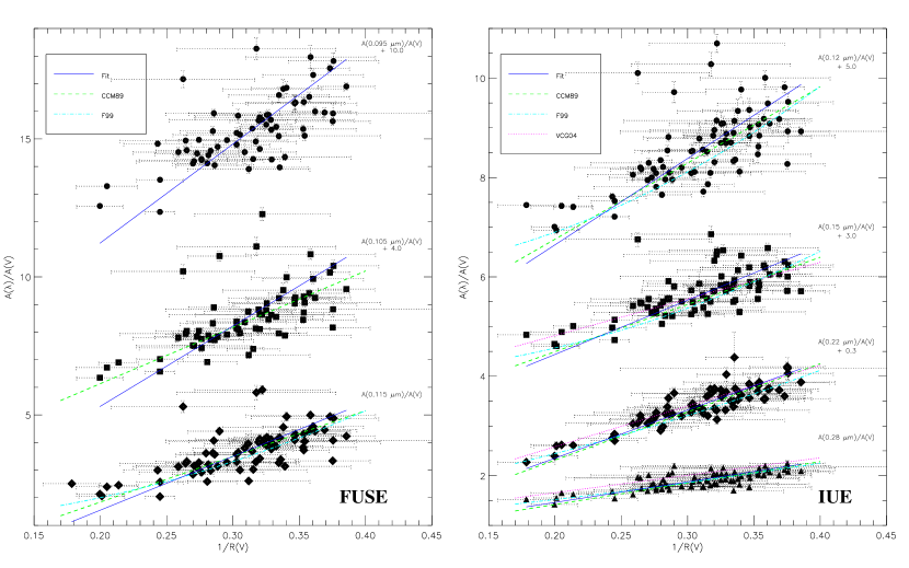
Figure 7.— The relationship between $A(\lambda)/A(V)$ and $R(V)^{-1}$ is shown for selected wavelengths using FUSE (left) and IUE (right). The relationships given by the CCM89 ($\lambda<10~{}\micron^{-1}$), F99 ($\lambda<8.7~{}\micron^{-1}$), and VCG04 ($\lambda<8~{}\micron^{-1}$) fits are also shown, but only for wavelengths for which they are valid. The IUE plot is similar to that of Fig. 1a of CCM89. The F99 relationship is non-linear in this form as it is based on correlations between FM90 fit parameters and $R(V)^{-1}$.

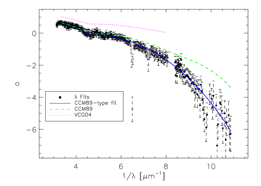
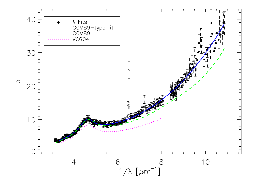
Figure 8.— The intercept (a) and slope (b) coefficients to the fits of $A(\lambda)/A(V)$ versus $R(V)^{-1}$ are plotted versus wavelength. Only fits using 40 or more points are plotted. The coefficients for the individual fits ($\lambda$ fits) and the CCM89-type functional fit to them are shown. The coefficients from CCM89 and VCG04 are also given for comparison. The regions around the wind lines (6.5 and 7.1 $\micron^{-1}$, open circles) are not used in the CCM89-like fit as they are almost never well matched by the comparison stars.

The work of CCM89 demonstrated that on average extinction curves follow a family of curves that can be described with one parameter. Real deviations from the CCM89 relationship exist and were studied by Mathis & Cardelli (1992) and VCG04. CCM89 chose $R(V)$ as the one parameter as it roughly measures the average grain size. The CCM89 relationship is an empirical relationship based on determining the linear correlation between $A(\lambda)/A(V)$ and $R(V)^{-1}$ at each wavelength with the resulting set of intercepts and slopes forming the the CCM89 $R(V)$ dependent relationship. The CCM89 relationship was constructed mainly using Fitzpatrick & Massa (1988) fits to IUE extinction curves and broadband data in the near-infrared and optical of 29 sightlines. This was supplemented with ANS UV photometry and Copernicus far-UV spectra for a smaller number of sightlines. The CCM89 relationship in the far-UV (8–10 $\micron^{-1}$) is mainly based on extrapolating the Fitzpatrick & Massa (1988) fits and represents the the most uncertain portion of the CCM89 relationship. Overall, CCM89 is valid from 0.3–10 $\micron^{-1}$ (3.3–0.1 $\micron$).

Since CCM89, there have been two other efforts to refine the R(V) dependent relationship in the ultraviolet (Fitzpatrick, 1999; Valencic et al., 2004). Fitzpatrick (1999) (hereafter F99) used the FM90 set of IUE extinction curves as the basis for their $R(V)$ dependent relationship. Their sample included 77 sightlines and the F99 relationship in the ultraviolet is based on the correlation between $C_{1}$ and $C_{2}$ FM90 coefficients and $R(V)^{-1}$ (the other coefficients are held constant). The near-IR and optical regions are fit using splines to account for the broad-band nature (and shifting effective wavelengths) of the data. The F99 relationship is valid from $\sim$0.2–8.7 $\micron^{-1}$ (5.0–0.115 $\micron$).

VCG04 used a sample of 417 IUE extinction curves as the basis for their $R(V)$ dependent relationship. They followed the methodology of CCM89 and fit $A(\lambda)/A(V)$ and $R(V)^{-1}$ at each wavelength. The resulting slopes and intercepts were fit with the same functional form as CCM89. This work concentrated on the IUE UV region and this is only valid between 3.3–8.0 $\micron^{-1}$ (0.3–0.125 $\micron$).

Using our sample of 75 FUSE extinction curves we can investigate the $R(V)$ dependent relationship in the far-UV (8.4–11 $\micron^{-1}$). We start by following the CCM89 methodology and perform fits of the data to

$$\frac{A(x)}{A(V)}=a(x)+\frac{b(x)}{R(V)}$$ (11)

where $x=\lambda^{-1}$. For consistency, we have determined the linear fit coefficients for both our FUSE and IUE extinction curves as this allows us to directly compare our $R(V)$ dependent relationship to the CCM89, F99, and VCG04. Unlike CCM89, we perform our linear fits on the actual extinction curves, not the FM90 fits. This directly connects our $R(V)$ relationship to the data and does not assume a functional form for the UV extinction curve. The linear fits are done using the ’fitexy’ IDL program that takes into account uncertainties on both the independent and dependent variables. Another approach was taken in deriving the $R(V)$ dependent relationship by F99 who correlated the FM90 parameters with $R(V)$. We did a similar analysis and found, just as F99 did, that most of the dependence of the extinction curves on $R(V)$ is due to correlations with $C_{1}$ and $C_{2}$. We choose to use the CCM89 methodology for our $R(V)$ relationship as it imposes fewer assumptions about the detailed structure of the relationship. Both approaches (CCM89 or F99) produce very similar $R(V)$ relationships.

The fit relationships, fits, and comparisons to previous $R(V)$ dependent relationships are shown in Fig. 7. The relationship shown by our sample of sightlines is similar to those seen in previous works, but our fits display a stronger dependence on $R(V)^{-1}$. In addition, our $R(V)$ dependent relationship is well defined all the way to 11 $\micron^{-1}$. As can be seen from this figure, our $R(V)$ dependent relationship is valid for $R(V)$ values between 2.5 and $\sim$5. The intercept (a) and slope (b) values are shown as a function of wavelength in Fig. 8 along with the values from previous works. We find quite different values for a and b compared to previous works and this illustrates that the values of a and b are not independent given that the differences between the different works are not nearly as striking in Fig. 7. As a check of the use of extrapolated FM90 parameters to deredden the comparison stars (§2.1), we have verified that the linear fits at each wavelength do not change significantly even when sightlines with lower reddenings are excluded from the fit (up to $A(V)=1.5$).

We fit our $a(x)$ and $b(x)$ values using a similar functional form as given by CCM89. Given that we have seen in this work that the FM90 parameterization of the far-ultraviolet ($x>5.9~{}\micron^{-1}$) provides a good representation of extinction curves to $x=11~{}\micron^{-1}$, we have expanded the term used by CCM89 to represent $3.3~{}\micron^{-1}\leq x\leq 8~{}\micron^{-1}$ to represent the entire range from $3.3~{}\micron^{-1}\leq x\leq 11~{}\micron^{-1}$. The term CCM89 used for $8~{}\micron^{-1}\leq x\leq 11~{}\micron^{-1}$ was an extrapolation of the FM90 far-UV term. Thus, for the entire wavelength range considered in this paper ($3.3~{}\micron^{-1}\leq x\leq 11~{}\micron^{-1}$) the functional form we use for our $R(V)$ dependent relationship is

$$a(x) = 1.896-0.372x-0.0108/[(x-4.57)^{2}+0.0422]$$ (12)

$$+F_{a}(x)$$

$$b(x) = -3.503+2.057x+0.718/[(x-4.59)^{2}+0.0530]$$ (13)

$$+F_{b}(x)$$

where for ($5.9\leq x\leq 8$)

$$F_{a}(x) = -0.110(x-5.9)^{2}-0.0099(x-5.9)^{3}$$ (14)

$$F_{b}(x) = 0.537(x-5.9)^{2}+0.0530(x-5.9)^{3}$$ (15)

and for ($x<5.9$)

$$F_{a}(x)=F_{b}(x)=0.$$ (16)

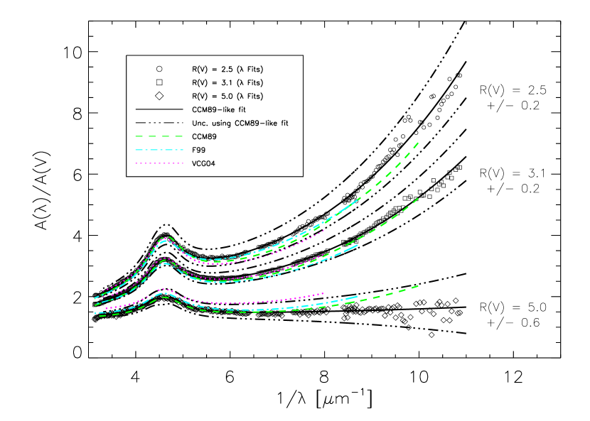
Figure 9.— The average extinction curves for $R(V)$ values of 2.5, 3.1, and 5.0 are shown. The new average curves derived in this paper are shown as well as those from CCM89, F99, and VCG04. The uncertainty on our $R(V)$ dependent relationship (i.e., $a(x)$ and $b(x)$) is shown using the $R(V)$ dependent fit that best describes the behavior of the uncertainties on the fits at each individual wavelength. In general, the fit uncertainties translate to an equivalent uncertainty of approximately 10% on $R(V)$.

We compare the average curves calculated from our newly derived $R(V)$ dependent relationship with those given by CCM89, F99, and VCG04 in Fig. 9. The $R(V)$ dependent relationship we derive is not noiseless and we show the uncertainties on the average curves to illustrate this point. The uncertainties on the curves resulting from uncertainties on $a(x)$ and $b(x)$ can be approximated by uncertainties on the value of $R(V)$. Overall, these uncertainties are equivalent to approximately a 10% error on $R(V)$. The uncertainties are significant and grow with decreasing wavelength. Overall, our new $R(V)$ dependent relationship is roughly consistent within our uncertainties with past measurements in areas of common wavelength coverage. But, over most of the ultraviolet we do find a stronger dependence on $R(V)$ than previous works. The statistically significance of this stronger dependence is difficult to assess given that previous works did not include an analysis of the uncertainties in their derivations of the $a(x)$ and $b(x)$. For VCG04, some of the differences can be traced to this study using unweighted linear least square fits to determine $a(x)$ and $b(x)$. We checked this effect and found much shallower $R(V)$ dependences with our sample if we perform unweighted fits. Taking into account the uncertainties on both $A(\lambda)/A(V)$ and $R(V)$ is clearly important. For CCM89 and F99, the largest differences are seen for $x>7~{}\micron^{-1}$ where we find a stronger dependence on $R(V)$. This is not surprising as only with this new work has this wavelength range been systematically studied.

3.4. Structure

The existence of structure in the UV extinction curve can give strong clues to the carriers of different dust grain components. The main UV absorption feature is the broad 2175 Å bump which has been identified with carbonaceous grains (Stecher & Donn, 1965; Draine & Malhotra, 1993). The other main structure is the far-UV rise and this feature is also identified (but with less confidence) with carbonaceous grains (Joblin et al., 1992; Li & Draine, 2001). Other than these two features, no other convincing UV features have been found. Clayton et al. (2003a) has presented the most sensitive search for UV absorptions to date. They observed two heavily reddened sightlines and derived a 3$\sigma$ upper limit of $\sim$$0.02A(V)$ on any features 20 Å or wider. This result has been strengthened by Fitzpatrick & Massa (2007) who found a 3$\sigma$ upper limit of $\sim$$0.06A(V)$ on features 10 Å or wider from the average residuals of 318 extinction curves.

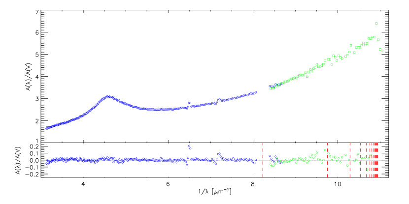
Figure 10.— The average extinction curve for the entire sample of 75 sightlines is plotted along with the average residual curve at a resolution of 250. The average residual curve was created by averaging the 75 individual observed minus FM90 fit curves. The deviations seen at 6.5 and 7.5 µm^-1 are the result of ISM or wind line mismatches.

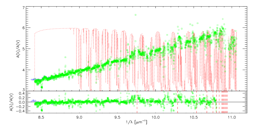
Figure 11.— The average extinction curve for the entire sample of 75 sightlines is plotted along with the average residual curve at a resolution of $10^{4}$. Overplotted on the average extinction curve is the $H_{2}$ and H I absorption spectrum (dotted line) for HD 122879 ($A(V)=1.41,R(V)=3.17$) to provide a guide to where strong $H_{2}$ and H I absorptions occur. The average residual curve was created by averaging 75 individual observed minus FM90 fit curves. Overplotted on the residual plot as dashed vertical lines is the location of the H I absorption features.

We have used our sample of 75 FUSE extinction curves to search of structure in the far-UV region. Fig. 10 presents the average extinction curve and residual curve for the entire sample at a spectral resolution of 250. There are two obvious features in the IUE spectral region and these correspond to either ISM or wind line mismatches between the reddened and comparison stars. There are no obvious features in the FUSE spectral region other than the scatter getting larger around $x=9.25~{}\micron^{-1}$ and then getting much larger after $x=10.75~{}\micron^{-1}$. The scatter of the FUSE residuals puts a 3$\sigma$ upper limit of $\sim$$0.12A(V)$ on features with a resolution of 250 ($\sim$4 Å width). For comparison to previous studies, our 3$\sigma$ upper limit in the IUE range is $\sim$$0.04A(V)$ on features with a resolution of 250 ($\sim$8 Åwidth).

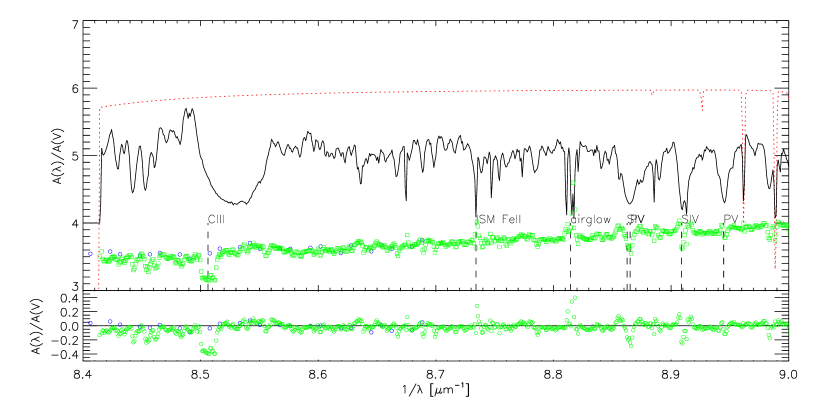
Figure 12.— The average extinction curve for $8.4<\lambda^{-1}<9.0~{}\micron^{-1}$ for the entire sample of 75 sightlines is plotted along with the average residual curve at a resolution of $10^{4}$. Overplotted on the average extinction curve is the spectrum of HD 122879 and the $H_{2}$ and H I absorption spectrum for this sightline ($A(V)=1.41,R(V)=3.17$). The average residual curve was created by averaging 75 individual observed minus FM90 fit curves. The locations of features that produce residuals in the average extinction curve are labeled.

We can also search for features at significantly higher resolution given that the native resolution of our FUSE spectra are on order $10^{4}$. Fig. 11 presents the average FUSE extinction curve and residual curve for the entire sample at a spectral resolution of $10^{4}$. There are a number of features in the residual curve. These features can be seen to correlate with strong absorptions in the example $H_{2}$ and H I absorption spectrum. For example, two of the largest deviations correspond to Ly$\beta$ and Ly$\gamma$ at 9.76 and 10.29 µm^-1, respectively. In addition, there is a strong residual at $\sim$10.15 µm^-1 that corresponds to a particularly strong $H_{2}$ absorption complex. In general, all of the strong residuals in the region beyond 8.9 µm^-1 correspond to regions of strong H I or $H_{2}$ absorption. There are residuals at $x<9~{}\micron^{-1}$ that are not associated with H I or $H_{2}$ absorptions. Fig. 12 shows a blowup of this wavelength region including the spectrum of HD 122879 as a guide to the origin of the stronger residuals. The strong residuals all correspond to strong stellar (C III, S IV, and P V), ISM (Fe II), or airglow lines (Pellerin et al., 2002). Examining Fig. 11, the scatter of the FUSE full resolution residuals clearly becomes large where $x\sim 9.6~{}\micron^{-1}$. Thus, the 3$\sigma$ upper limits are $\sim$$0.15A(V)$ for $x<9.6$ µm^-1 and $\sim$$0.68A(V)$ for $x>9.6$ µm^-1 on features with a resolution of $10^{4}$ ($\sim$0.1 Å width).

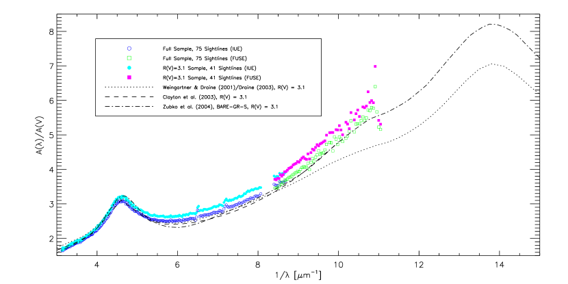
Figure 13.— The average extinction curve for the 41 curves in the sample that have $R(V)$ values within $1\sigma$ of 3.1 is shown at a resolution of 250. The $R(V)=3.1$ models from Weingartner & Draine (2001), Clayton et al. (2003b), and Zubko et al. (2004) are plotted for comparison. Note that the Clayton et al. (2003b) model only extends to $10~{}\micron^{-1}$.

The average far-UV extinction curve can be compared with existing dust grain models to evaluate how well such grain models do at describing and/or predicting the far-UV extinction. The comparison is shown in Fig. 13 where we show the average of all 75 sightlines (same as in Figs. 10 & 11) and the average of the 41 sightlines that have $R(V)$ values within $1\sigma$ of 3.1. The average $R(V)$ for the full sample is 3.33 while the average for the $R(V)=3.1$ sample of 41 sightlines is, not surprisingly, 3.13. In addition to the observed average curves, three different dust grain models (Weingartner & Draine, 2001; Clayton et al., 2003b; Zubko et al., 2004) are shown in this figure. These models used different constraints and methods to determine the dust grain size distribution and have known differences as a result. While all of the dust grain models shown are for an $R(V)=3.1$ (diffuse ISM), they are in closer agreement with the average for our full sample than the $R(V)=3.1$ average. This difference can be mainly traced to the differences seen between our work and previous determinations of the $R(V)$ dependent relationship. Weingartner & Draine (2001) and Zubko et al. (2004) used the $R(V)=3.1$ curve from F99 while Clayton et al. (2003b) used the $R(V)=3.1$ curve from CCM89. As both the CCM89 and F99 $R(V)=3.1$ curves are below our $R(V)=3.1$ determined from the $R(V)$ dependent relationship (see Fig. 9), it is not surprising the dust grain models are also below our curve. The differences between the CCM89, F99, and this work are due to different samples of extinction curves used as well as different fitting approaches. The Clayton et al. (2003b) and Zubko et al. (2004) models do a much better job in reproducing the far-UV extinction levels than the Weingartner & Draine (2001) (as updated by Draine, 2003) model. Overall, the far-UV rise seems to consistent with its potential origin as a second resonance feature centered around 14 $\micron^{-1}$ (Joblin et al., 1992; Li & Draine, 2001).

4. Conclusions

We have presented FUSE+IUE extinction curve for 75 sightlines that have $A(V)$ values from 0.6 to 3.2 mag. The $R(V)$ values of this sample range from 2.5 to 5.5 with a strong clustering around 3. These extinction curves were created using the standard pair method. Given the FUSE sensitivities, this required generating a new set of unreddened comparison stars. This set of 75 FUSE extinction curves represents a large increase in the number of extinction curves well measured in the far-ultraviolet.

Using this sample, we investigated the nature of the far-UV extinction with three methods. The first was to fit all the curves with the FM90 parameterization. We found that the FM90 parameters determined with just the IUE portion of the extinction curve to be broadly consistent with those that were determined using the FUSE+IUE extinction curves. There were significant changes in the individual values of the $C_{4}^{A(V)}$ and $\gamma$ parameters. In addition, the average $C_{4}^{A(V)}$ parameter decreased by $\sim$8% indicating that the strength of the far-UV rise is overestimated when using only IUE data. All the extinction curves had positive far-UV rises when fit with the FUSE+IUE data giving no indication that the far-UV rise was turning over at the shortest wavelengths. We tested the new FM07 parameterization (with 1 additional parameter and a simplified far-UV rise term) using the combined FUSE+IUE curves and found only a weak preference for the FM07 parameterization. We choose to use the FM90 parameterization as it is simpler and provides for direct comparisons to previous work.

The second investigation of the far-UV extinction concentrated on deriving the $R(V)$ dependent relationship. We derived the linear dependence of $A(\lambda)/A(V)$ on $R(V)^{-1}$ at each FUSE and IUE wavelength including the observational uncertainties as part of the fitting. We found a stronger dependence of $A(\lambda)/A(V)$ on $R(V)^{-1}$ than previously indicated in the far-UV. It is not surprising as the previous work in the far-UV was based on only a very limited number of sightlines. We include the uncertainties in the fit in the $R(V)$ dependent parameterization and find that our derivation is broadly consistent with previous work (Cardelli et al., 1989; Fitzpatrick & Massa, 1999; Valencic et al., 2004) in the regions of overlap (mainly the IUE range). We present our $R(V)$ dependent relationship for the entire UV ($3.3~{}\micron^{-1}\leq\lambda^{-1}\leq 11~{}\micron^{-1}$) using the same functional form as used by CCM89.

Finally, we searched for discrete absorption features in the far-UV. We looked for features at a resolution of 250 by averaging all 75 extinction curves and also averaging the residuals of each curve from its corresponding FM90 fit. We find a 3$\sigma$ upper limit of $\sim$$0.12A(V)$ on features with a resolution of 250 ($\sim$4 Å width). Utilizing the high spectral resolution nature of the FUSE observations, we also searched for features at the native resolution of $10^{4}$. We found 3$\sigma$ upper limits of $\sim$$0.15A(V)$ for $\lambda^{-1}<9.6$ µm^-1 and $\sim$$0.68A(V)$ for $\lambda^{-1}>9.6$ µm^-1 on features with a resolution of $10^{4}$ ($\sim$0.1 Å width).

References

- Cardelli et al. (1989) Cardelli, J. A., Clayton, G. C., & Mathis, J. S. 1989, ApJ, 345, 245
- Cardelli et al. (1992) Cardelli, J. A., Sembach, K. R., & Mathis, J. S. 1992, AJ, 104, 1916
- Cartledge et al. (2009) Cartledge, S. I. B., Clayton, G. C., & Gordon, K. D. 2009, in prep
- Cartledge et al. (2005) Cartledge, S. I. B., et al. 2005, ApJ, 630, 355
- Clayton et al. (2003a) Clayton, G. C., et al. 2003a, ApJ, 592, 947
- Clayton et al. (2003b) —. 2003b, ApJ, 588, 871
- Draine (2003) Draine, B. T. 2003, ARA&A, 41, 241
- Draine & Malhotra (1993) Draine, B. T. & Malhotra, S. 1993, ApJ, 414, 632
- Fitzpatrick (1999) Fitzpatrick, E. L. 1999, PASP, 111, 63
- Fitzpatrick & Massa (1986) Fitzpatrick, E. L. & Massa, D. 1986, ApJ, 307, 286
- Fitzpatrick & Massa (1988) —. 1988, ApJ, 328, 734
- Fitzpatrick & Massa (1990) —. 1990, ApJS, 72, 163
- Fitzpatrick & Massa (1999) —. 1999, ApJ, 525, 1011
- Fitzpatrick & Massa (2005) —. 2005, AJ, 130, 1127
- Fitzpatrick & Massa (2007) —. 2007, ApJ, 663, 320
- Flaherty et al. (2007) Flaherty, K. M., et al. 2007, ApJ, 663, 1069
- Gordon & Clayton (1998) Gordon, K. D. & Clayton, G. C. 1998, ApJ, 500, 816
- Gordon et al. (2003) Gordon, K. D., et al. 2003, ApJ, 594, 279
- Herbig (1995) Herbig, G. H. 1995, ARA&A, 33, 19
- Indebetouw et al. (2005) Indebetouw, R., et al. 2005, ApJ, 619, 931
- Joblin et al. (1992) Joblin, C., Leger, A., & Martin, P. 1992, ApJ, 393, L79
- Li & Draine (2001) Li, A. & Draine, B. T. 2001, ApJ, 554, 778
- Martin & Whittet (1990) Martin, P. G. & Whittet, D. C. B. 1990, ApJ, 357, 113
- Massa et al. (1983) Massa, D., Savage, B. D., & Fitzpatrick, E. L. 1983, ApJ, 266, 662
- Mathis & Cardelli (1992) Mathis, J. S. & Cardelli, J. A. 1992, ApJ, 398, 610
- Merrill (1934) Merrill, P. W. 1934, PASP, 46, 206
- Moos et al. (2000) Moos, H. W., et al. 2000, ApJ, 538, L1
- Pellerin et al. (2002) Pellerin, A., et al. 2002, ApJS, 143, 159
- Rieke & Lebofsky (1985) Rieke, G. H. & Lebofsky, M. J. 1985, ApJ, 288, 618
- Rieke et al. (1989) Rieke, G. H., Rieke, M. J., & Paul, A. E. 1989, ApJ, 336, 752
- Sofia et al. (2005) Sofia, U. J., et al. 2005, ApJ, 625, 167
- Stecher (1965) Stecher, T. P. 1965, ApJ, 142, 1683
- Stecher (1969) —. 1969, ApJ, 157, L125+
- Stecher & Donn (1965) Stecher, T. P. & Donn, B. 1965, ApJ, 142, 1681
- Valencic et al. (2004) Valencic, L. A., Clayton, G. C., & Gordon, K. D. 2004, ApJ, 616, 912
- Weingartner & Draine (2001) Weingartner, J. C. & Draine, B. T. 2001, ApJ, 548, 296
- Zubko et al. (2004) Zubko, V., Dwek, E., & Arendt, R. G. 2004, ApJS, 152, 211