Finite Difference-Time Domain solution of the Dirac equation and the dynamics of the Aharonov-Bohm effect

Abstract

The time-dependent Dirac equation is solved using the three-dimensional Finite Difference-Time Domain (FDTD) method. The dynamics of the electron wave packet in a vector potential is studied in the arrangements associated with the Aharonov-Bohm effect. The solution of the Dirac equation showed a change in the velocity of the electron wave packet even in a region where no forces acted on the electron. The solution of the Dirac equation agreed with the prediction of classical dynamics under the assumption that the dynamics was defined by the conservation of generalized or canonical momentum. It was also shown that in the case when the magnetic field was not zero, the conservation of generalized or canonical momentum was equivalent to the action of the Lorentz force.

1 Introduction

In our previous papers [1, 2], the Finite Difference-Time Domain (FDTD) method, originally introduced by Kane Yee [3] to solve Maxwell’s equations, was for the first time applied to solve the three-dimensional Dirac equation. The $Zitterbewegung$ and the dynamics of a well-localized electron were used as examples of FDTD applied to the case of free electrons. The motion of electron wave packets inside and scattering from the potential step barrier or linearly dependent potential, arrangements associated with the Klein paradox [4], were used as examples of interaction with a scalar potential. In this paper, a FDTD study of the dynamics of an electron wave packet under the influence of a vector potential is presented. Such a dynamic behavior is most often associated with the Aharonov-Bohm effect [5].

As a manifestation of quantum mechanics, charged particles passing around a long solenoid can feel a magnetic flux even when all the fields in the region through which the particles travel are zero. The shifts in the phase of the wave functions describing the particles have been experimentally verified by its effect on the interference fringes [6, 7, 8, 9]. Since, classically, there are no forces acting on the charged particles in the zero field region, the theoretical description of the Aharonov-Bohm effect contains a number of assumptions. They include assumptions on nonlocal features of quantum mechanics, the physical meaning of the vector potential, topological effects, etc. Generally accepted physical understanding is still lacking [10]. While there is still an open question on the presence of classical forces responsible for the Aharonov-Bohm effect [10, 11, 12], on a macroscopic level they have not been observed [13].

Proper quantum-mechanical description of the dynamics of a relativistic charged particle involves the solution of the Dirac equation in the time domain. In addition to initial conditions, such a dynamics is defined only by the configuration of the scalar and vector potentials, and does not involve knowledge or any assumption on “classical forces”. The solutions of the time-dependent Dirac equation, some of which are presented in this paper, can shed light and fill critical knowledge gaps on the theoretical and experimental interpretations of the mechanism of the Aharonov-Bohm effect, including the existence or non-existence of classical forces.

2 Time-dependent solution of the Dirac equation

The FDTD solutions of the time-dependent Dirac equation were obtained for the case when the electromagnetic field described by the four-potential ${A^{\mu}=\{A_{0}(x),\vec{A}(x)\}}$ was minimally coupled to the particle [14, 15]

$${\imath\hbar{\frac{\partial\Psi}{\partial t}}=({H}_{free}+{H}_{int})\Psi},$$ (1)

where

$${{H}_{free}=-\imath c\hbar{{\bf\alpha}\cdot\nabla}+\beta mc^{2}},$$ (2)

$${{H}_{int}=-e{{\bf\alpha}\cdot{\vec{A}}}+eA_{0}},$$ (3)

and

$${\Psi(x)=\left(\begin{array}[]{c}\Psi_{1}(x)\\ \Psi_{2}(x)\\ \Psi_{3}(x)\\ \Psi_{4}(x)\end{array}\right)}.$$ (4)

The matrices ${\bf\alpha}$ and $\beta$ were expressed using $2\times 2$ Pauli matrices $\bf\sigma^{{}^{\prime}}s$ and the $2\times 2$ unit matrix $I$.

In the FDTD method, the time dependent solution of the Dirac equation was obtained using updating difference equations [1]. As an example, the values of $\Psi_{1}$ at the position $(i\Delta x,j\Delta y,k\Delta z)$ and at the time step $(n+1/2)\Delta t$ were obtained using the equation

$$\Psi_{1}^{n+1/2}(I,J,K) = \frac{2-C^{n}(I,J,K)}{C^{n}(I,J,K)}\Psi_{1}^{n-1/2}(I,J,K)$$ (5)

$$- {\frac{c\Delta t}{2\Delta xC^{n}(I,J,K)}}[\Psi_{3}^{n}(I,J,K+1)-\Psi_{3}^{n}(I,J,K-1)$$

$$+ \Psi_{4}^{n}(I+1,J,K)-\Psi_{4}^{n}(I-1,J,K)-i(\Psi_{4}^{n}(I,J+1,K)$$

$$- \Psi_{4}^{n}(I,J-1,K))]+i{\frac{e\Delta t}{\hbar C^{n}(I,J,K)}}[A^{n}_{1}(I,J,K)\Psi_{4}^{n}(I,J,K)$$

$$- iA^{n}_{2}(I,J,K)\Psi_{4}^{n}(I,J,K)+A^{n}_{3}(I,J,K)\Psi_{3}^{n}(I,J,K)],$$

where $C^{n}(I,J,K)=1+i\frac{\Delta t}{2\hbar}[mc^{2}+eA^{n}_{0}(I,J,K)]$. The space and time were discretized using uniform rectangular lattices of size $\Delta x$, $\Delta y$ and $\Delta z$, and uniform time increment $\Delta t$. While it is not generally required, in the Eq. (5) $\Delta x=\Delta y=\Delta z$. Updating equations for $\Psi_{2}$, $\Psi_{3}$, and $\Psi_{4}$ were constructed in a similar way.

The dynamics of a Dirac electron can now be studied in any environment described by a four-potential $A^{\mu}$ regardless of its complexity and time dependency. In this paper we studied the dynamics defined by the vector potential $\vec{A}(x)\neq 0$.

The Dirac equation is a differential equation of the first order and linear in $\partial/\partial t$. As in the case of Maxwell’s equations, the entire dynamics of the electron is defined, only by its initial wave function. The dynamics of a wave packet used in this paper was defined by the initial wave function of the form

$${\Psi(\vec{x},0)=N\sqrt{\frac{E+mc^{2}}{2E}}\left(\begin{array}[]{c}1\\ 0\\ \frac{p_{3}c}{E+mc^{2}}\\ \frac{(p_{1}+ip_{2})c}{E+mc^{2}}\end{array}\right)}e^{-\frac{\vec{x}\cdot\vec{x}}{4x_{0}^{2}}+\frac{i\vec{p}\cdot\vec{x}}{\hbar}},$$ (6)

where $N=[(2\pi)^{3/2}x_{0}^{3}]^{-1/2}$ is a normalizing constant. Eq. (6) represents a wave packet whose initial probability distribution is of a normalized Gaussian shape. Its size is defined by the constant $x_{0}$, its spin is pointed along the z-axis, and its motion is defined by the values of the momenta $p_{1},p_{2}$, and $p_{3}$. Some consequences of the initial localization of the wave packet on the overall dynamics of the electron were studied in Ref. [1, 16].

3 Validation of the computation: the dynamics of a wave packet in a strong uniform magnetic field

The dynamics of a wave packet is very complex. The dynamics of a particle described by the wave packet in Eq. (6) depends on its localization, defined by the Gaussian component of the wave function, and its initial momentum, part of the wave function’s phase. While an extensive study was done on the dynamics of the wave packet related to the scalar component $A_{0}(x)$ of a four-potential [2], such a study does not validate the dynamics of the wave packet related to the vector component of a four-potential $\vec{A}(x)$.

Applying the FDTD method to study the dynamics of a wave packet in a vector potential associated with a strong uniform magnetic field is not difficult. Classically, the dynamics consist of uniform rotational motion. In the relativistic quantum-mechanical description, however, even such a simple dynamics can validate the FDTD computation only up to a certain level. As pointed out in Ref. [17] ”the dynamics is particularly rich and not adequately described by semiclassical approximations”. In Ref. [18] it was demonstrated that in the presence of an external magnetic field the wave packet splits into two parts which rotate with different cyclotron frequencies, and after a few periods, the motion acquires irregular character. As a result of such a complex dynamics, when comparing the results obtained by the FDTD method and the computation described in Ref. [17] and [18], we could not expect more than a qualitative agreement. In addition to this qualitative agreement, of equal importance to the validation of the computation is the consistency of the results obtained for different vector potential gauges.

In this paper, the motion of the wave packet described by Eq. (6) was studied in a uniform magnetic field oriented along the y-axis

$$\vec{B}=(0,B_{0},0).$$ (7)

For this field the corresponding vector potential in a rotationally invariant gauge was

$$\vec{A}={B_{0}\over 2}(-z,0,x).$$ (8)

The dynamics of the wave packet was obtained by solving the Dirac equation for this vector potential.

While the probability densities $|\Psi|^{2}$ were calculated for the entire computational volume and at every time step, their values are shown here only on two planes, the horizontal or plane of classical particle motion, and the plane vertical to the plane of motion. The schematics of the planes relative to the wave packet motion and the orientation of the magnetic field are shown in Fig 1. The position and the shape of the wave packet in the horizontal plane, as it moves along its first orbit, is shown in Figure 2. The initial position of the wave packet was at the center of the vector potential. Its initial momentum was $p_{1}=0.53\;MeV/c$, making the motion relativistic. In order to force a relativistic electron to complete a full circle in the available computational space, the magnitude of the magnetic field was $B_{0}=10^{8}\;T$. The field of such a strength is associated with the fields at the surface of the neutron stars. The classical orbit of the electron in this field is $r_{class}=p_{1}/(eB_{0})=1.76\times 10^{-2}\;nm$. As shown in Figure 2, during the first rotation the wave packet generally follows the classical orbit and disperses at the same time. The position of the center of probability of the wave packet relative to the classical orbit is shown in Fig 3.

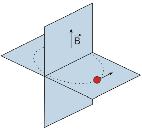
Figure 1: Schematics of the two planes used in displaying the probability densities. They are shown relative to the classical orbit of the electron and the orientation of the uniform magnetic field.

The complexity of the dynamics of the wave packet increased in the later stages of the motion. While the wave packet followed the circular motion, the probability density $|\Psi|^{2}$ at some times assumed the spiral shape shown in Figure 4, increased or reduced its length, changed its rotational motion, and translated from one place to another. Overall, the characteristics of this dynamics were similar to the characteristics described in Ref. [17] and [18]. While the figures show some of the complex shapes of the probability density $|\Psi|^{2}$, the richness of the electron motion can be better appreciated through the animation of the dynamics accessible on-line [19].

There was no intention of this validation to study the property of the confinement of the electron by the electrostatic potential. But, by using a scalar potential $A_{0}$ at the boundaries of the computational volume to limit the electron motion in the direction of the magnetic field, due to the wave packet dispersion, we have inadvertently also solved the Dirac equation for the confined electron. We reported [2] that, contrary to the claim of the Klein paradox, there was no penetration of the wave packet into a potential barrier of a supercritical potential of height $V$ satisfying the condition $eV>E+mc^{2}$. The time evaluation of the solution of the Dirac equation shown in Figure 5 confirms this result. Figure 5 shows that the electron wave function, as the wave packet disperses and reaches a non-penetrable electrostatic potential, creates a bound state. Reduction of number of nodes in a bound state solution could be interpreted as a transition of the particle from the higher energy state into the lover energy state as it orbits in a uniform magnetic field.

Several additional tests of the FDTD method were performed using the dynamics of the electron in the uniform magnetic field. As expected, due to the normal spin and the magnetic field orientation, reversal of the orientation of the magnetic field resulted in the reversal of the direction of the rotation of the wave packet, keeping the same properties of the dynamics of motion.

Of particular interest was testing the effects of the choice of gauge. The motion of the same wave packet was also studied for the uniform magnetic field oriented along the y-axis defined by the translationally invariant gauges

$$\vec{A}={B_{0}}(-z,0,0),$$ (9)

or

$$\vec{A}={B_{0}}(0,0,x).$$ (10)

In both cases the wave packet persisted in a circular motion following the classical orbit. While the dynamics of the wave packet behaved as expected, using translationally invariant gauges has an additional importance on validating the FDTD computation. As seen in Eq. (5), the gauge in Eq. (9) couples to the $\Psi_{4}$ component and the gauge in Eq. (10) couples to the $\Psi_{3}$ component. Similarly, the cross coupling exists for other components of the wave function $\Psi$. As a result, the same dynamics should be obtained by different combinatorics of the components of the vector potential and the components of the wave function. This enabled for testing of possible inconsistencies in the FDTD updating equations. No inconsistencies were found.

The dynamics of the wave packet motion in a uniform magnetic field was used here only as a validation of the FDTD method when a vector potential was applied in the Dirac equation. The same complexity of the quantum dynamics of motion as in previous publications [17, 18] was shown. While used here only for computational validation of the FDTD method, this dynamics could be studied as a separate problem in more detail in the future.

Finally, the complexity of the quantum dynamics of the wave packet in a uniform magnetic field studied here for three choices of gauge could be fully appreciated only by downloading the related animations [19].

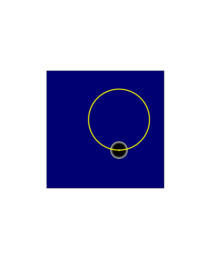
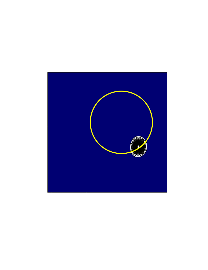
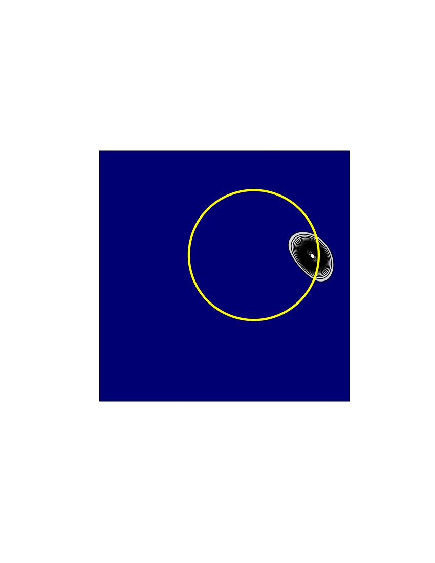
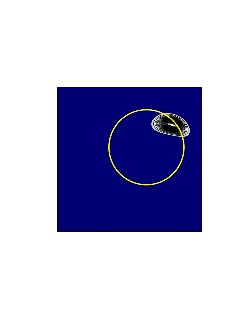
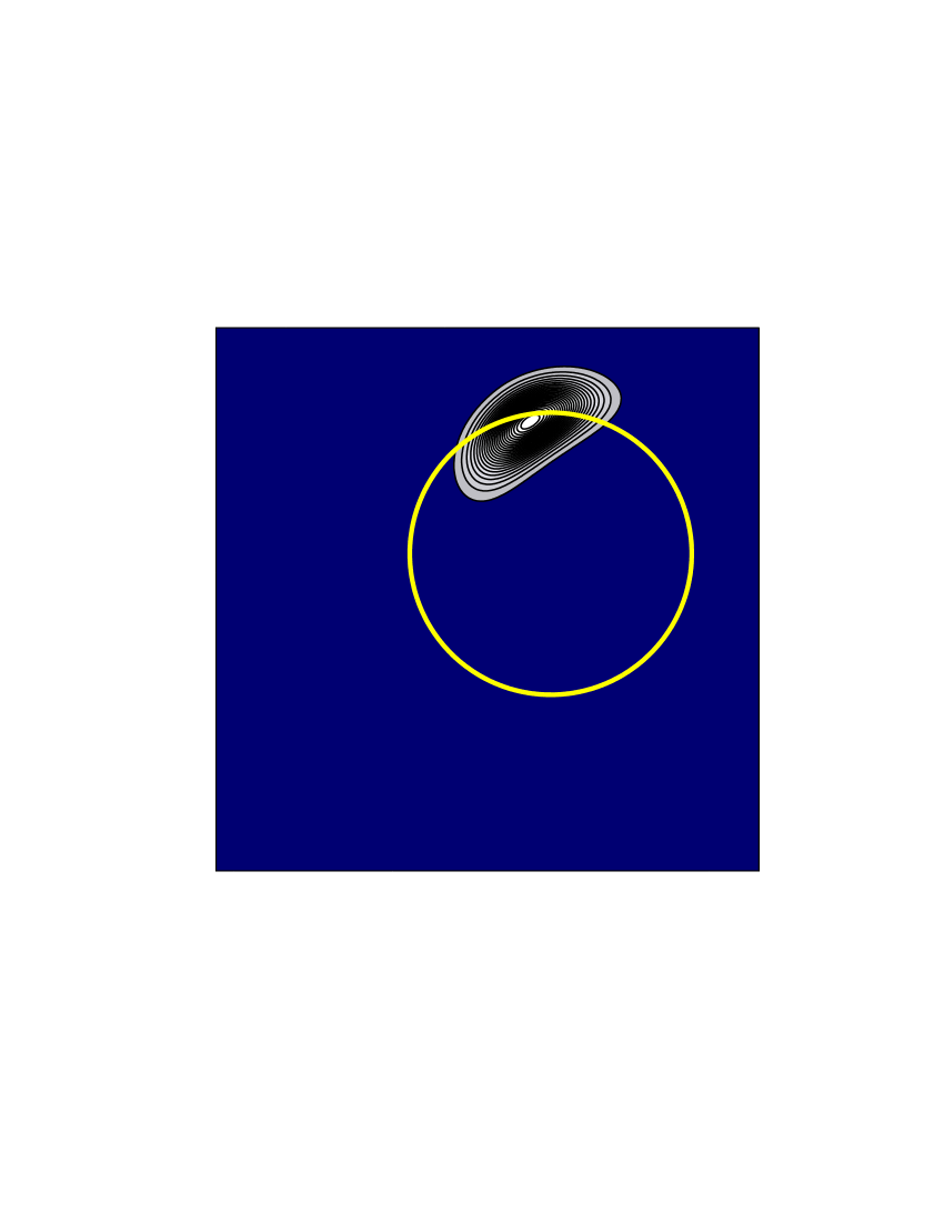
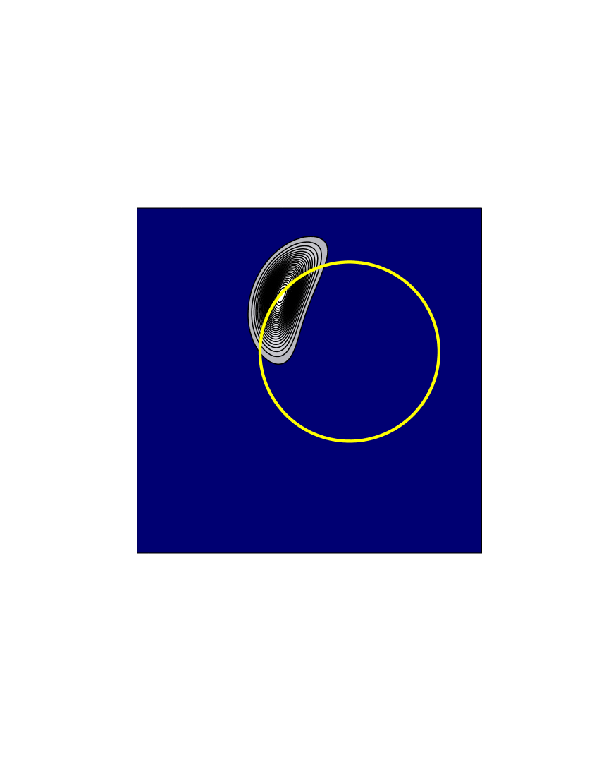
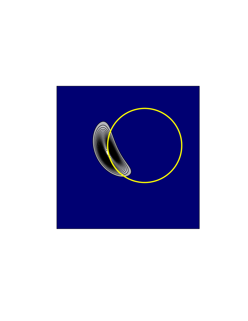
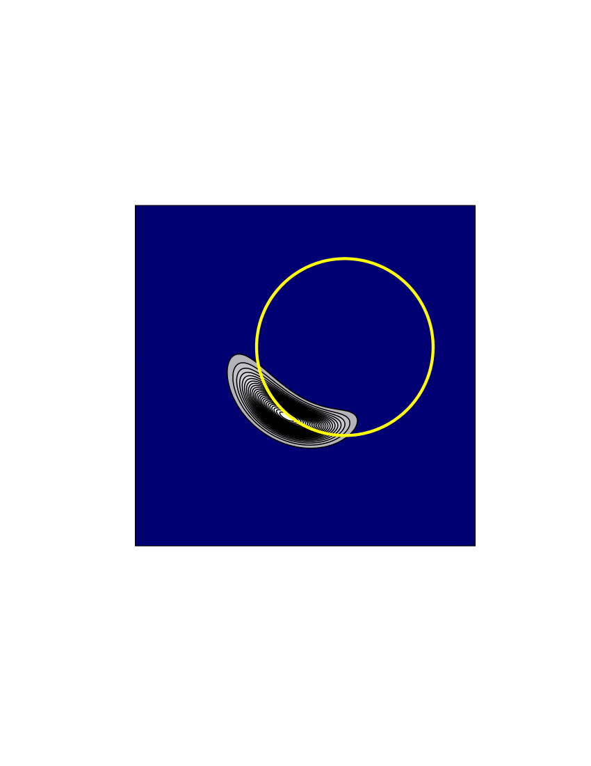
Figure 2: The shapes and the positions of the wave packet in the horizontal plane during the first rotation. The circle represents the classical orbit. The animation can be accessed on-line [19].

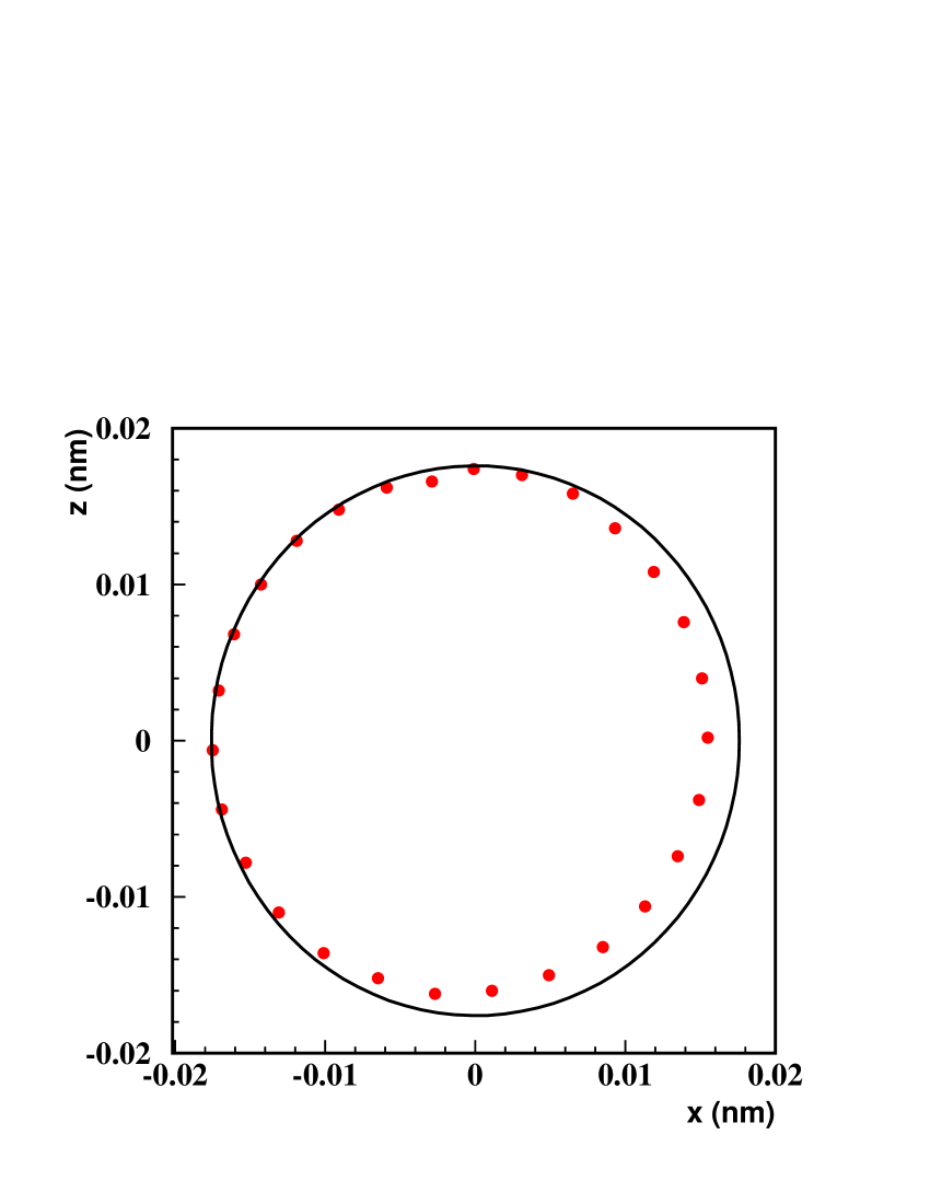
Figure 3: Positions of the center of probability of the wave packet in the horizontal plane during the first rotation. The circle represents the classical orbit. The animation of the dynamics can be accessed on-line [19].

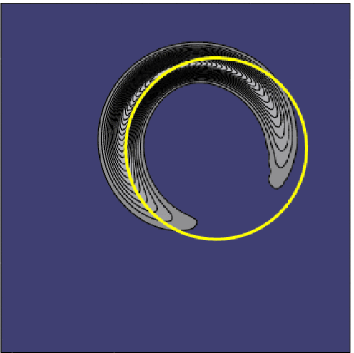
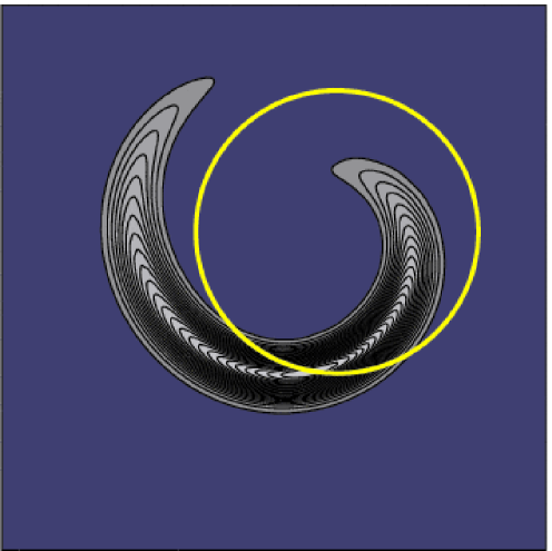
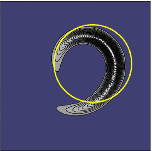
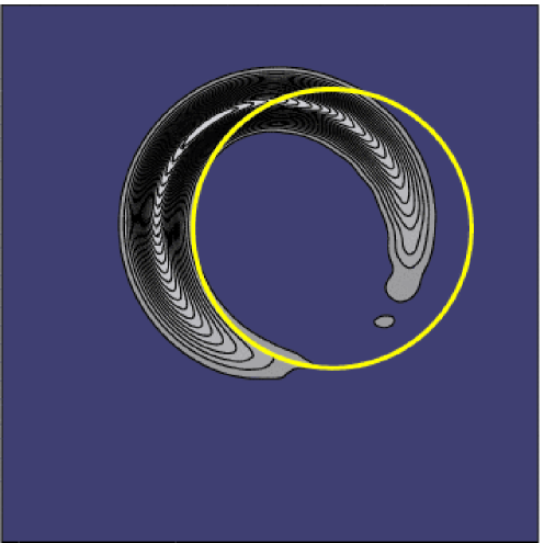
Figure 4: Changes in the shape of the probability density $|\Psi|^{2}$ during one of the subsequent orbits of the wave packet. The circle represents the classical orbit. The animation of the dynamics can be accessed on-line [19].

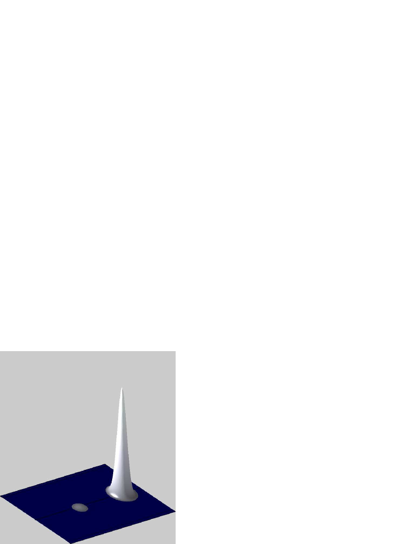
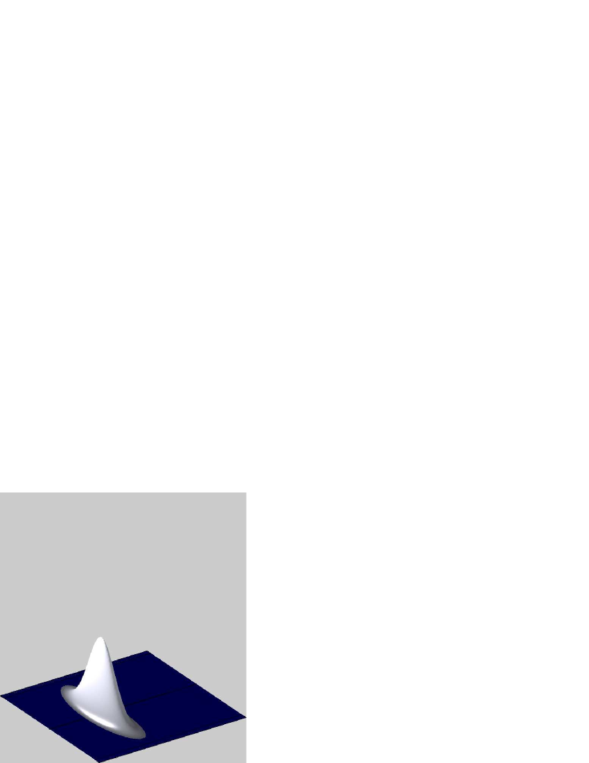
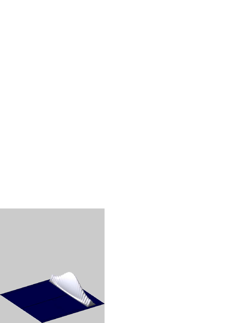
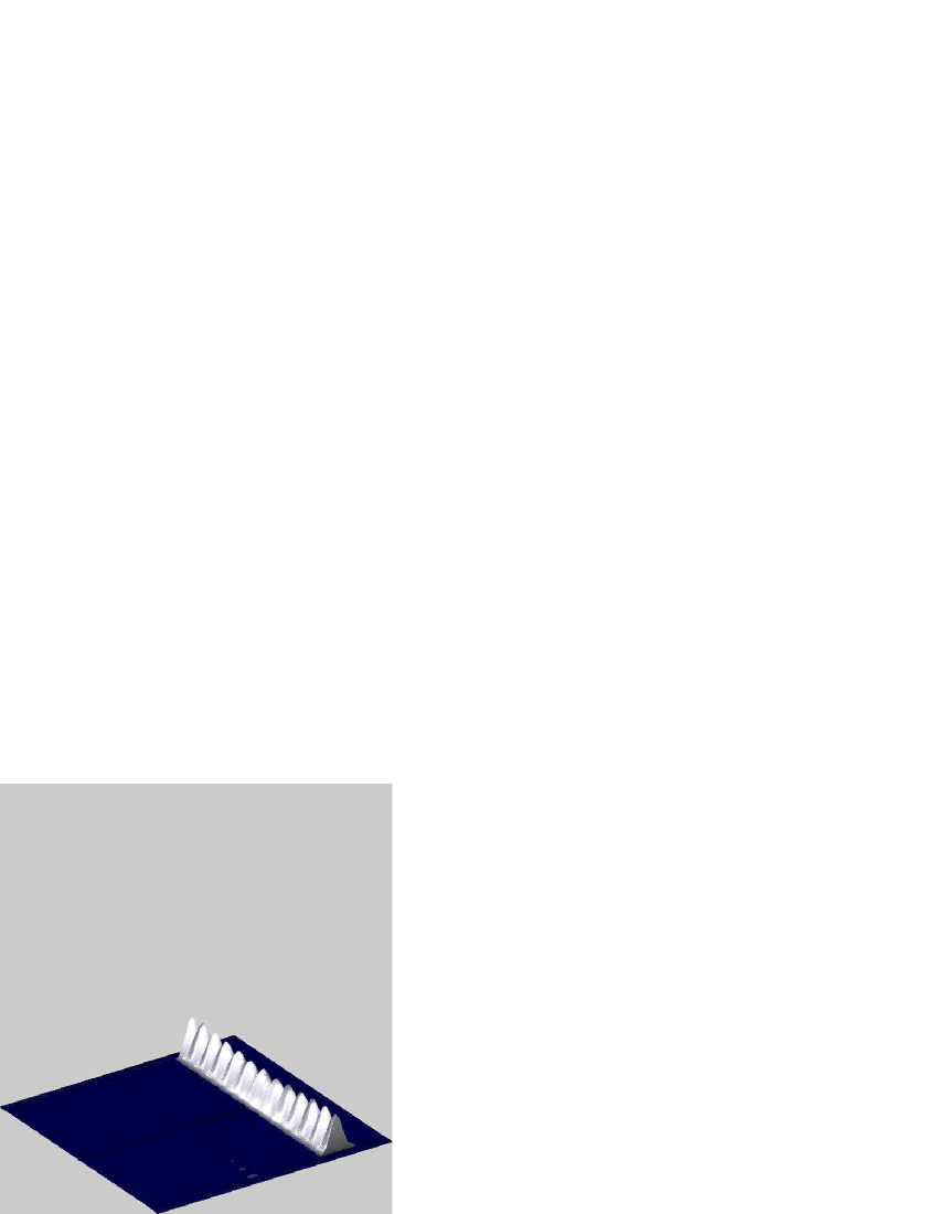
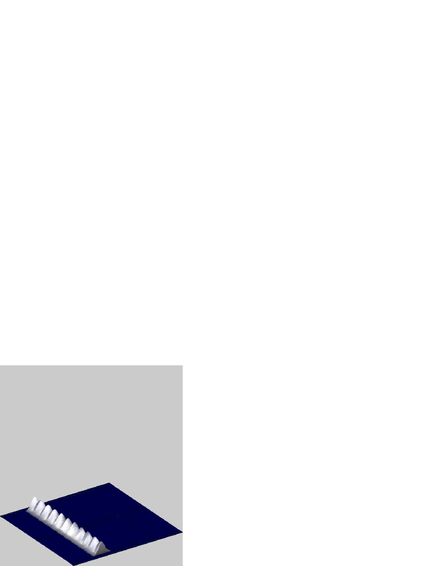
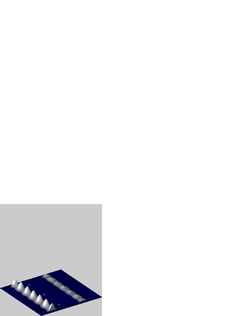
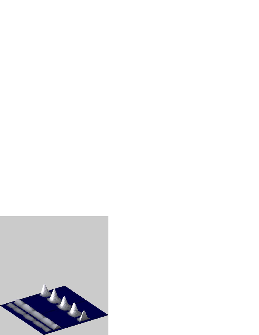
Figure 5: The shape of the probability density $|\Psi|^{2}$ in the vertical plane at the time when the wave packet crosses it. As the wave packet disperses and reaches the non-penetrable scalar potential $A_{0}$, the electron wave function creates a bound state in the direction of the magnetic field. As the wave packet rotates in the uniform magnetic field, the number of nodes reduces. The related animation can be accessed on-line [19].

4 Wave packet dynamics in a vector potential created by two infinite solenoids

The goal of this work is to study the dynamics of an electron wave packet under the influence of a vector potential associated with the Aharonov-Bohm effect [5]. Particularly, in this paper we present the dynamics of a wave packet obtained from the solution of the Dirac equation with a vector potential created by two infinite solenoids.

The vector potential of a single infinite solenoid oriented along the y-axis can be written as

$${\vec{A}=\left\{\begin{array}[]{c}{\Phi\over{2\pi R_{0}^{2}}}(-z,0,x)\;\;\;\;\;\mbox{ for $r\leq R_{0}$}\\ {\Phi\over{2\pi r^{2}}}(-z,0,x)\;\;\;\;\;\mbox{ for $r>R_{0}$}\end{array}\right.},$$ (11)

where $\Phi=B_{0}\pi R_{0}^{2}$ is the magnetic flux inside the solenoid, $B_{0}$ defines the strength of the magnetic field, $R_{0}$ is the radius of the solenoid, and $r=\sqrt{x^{2}+z^{2}}$ is the distance from the center of the solenoid in the x-z plane. Outside two parallel infinite solenoids separated by a distance $2a$ and with opposite magnetic field orientation, the vector potential is then

$$\!\!\!\!\!\!\!\!\!\!\!\!\!\!\!\!\!\!\vec{A}={\Phi\over{2\pi}}\left({{z+a}\over{x^{2}+(z+a)^{2}}}-{{z-a}\over{x^{2}+(z-a)^{2}}},0,{{x}\over{x^{2}+(z-a)^{2}}}-{{x}\over{x^{2}+(z+a)^{2}}}\right)\!.$$ (12)

An example of the shape of this potential is shown in Figure 6. Outside the solenoids, the associated magnetic fields $\vec{B}=\vec{\nabla}\times\vec{A}$ of the vector potentials described by Eqs. (11) and (12) are zero.

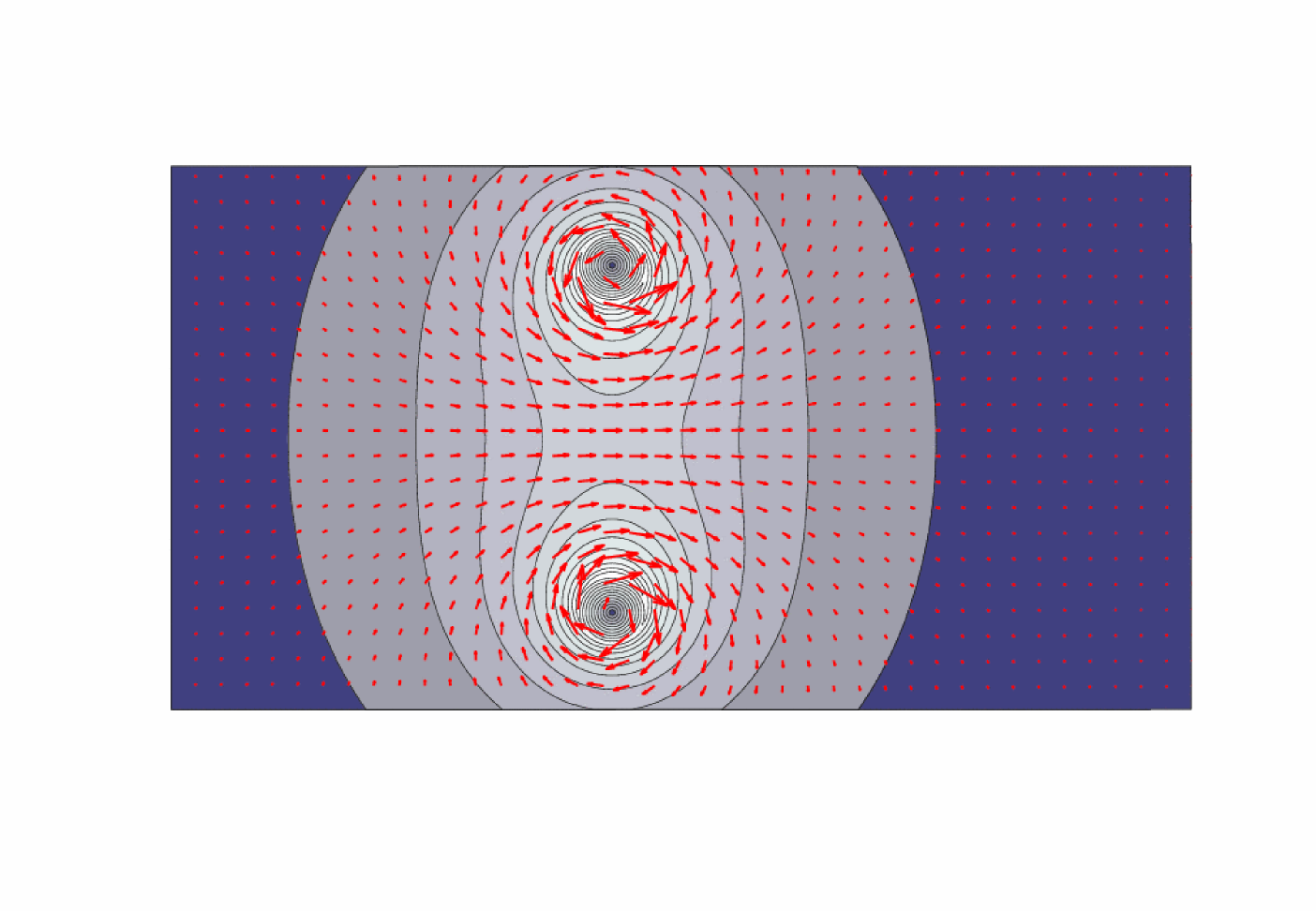
Figure 6: Vector potential of two parallel infinite solenoids with oppositely directed magnetic fluxes of the same magnitude. The potential is shown in the plane normal to the orientation of the solenoids.

The time-dependent Dirac equation is now solved for the scalar component of the four-potential $A_{0}=0$ and the vector component $\vec{A}$ defined by Eq. (12). With this choice we can study the dynamics of the wave packet in the region where the electric and the magnetic fields are zero. Obviously, in this region the Lorentz force acting on the electron, $\vec{F}=e(\vec{E}+\vec{v}\times\vec{B})$, is also zero.

The dynamics of the electron motion between two infinite and parallel solenoids is essentially the same as the electron dynamics in the case of Aharonov-Bohm effect. In both cases the electron moves in a field free region with no Lorentz force acting on it. Because of the symmetry, however, the dynamics in the case of two infinite solenoids consists only of the motion along one straight line between the solenoids. This avoids the complications of the Aharonov-Bohm dynamics where the trajectories on opposite sides of a single solenoid are compared. Because the properties of the dynamics are not studied through an interference, in the case of two solenoids the changes in the dynamics of the electron wave packet exclude the contribution of the nonlocal properties of the electron wave function dependent on the topology of the space. Another advantage of using two solenoids and localized wave packet is the possibility to separate the solenoids far enough that no parts of the wave packet penetrate the non-zero field region inside the solenoids, excluding this contribution to the dynamics as well. If necessary, the solenoids could be shielded by a potential barrier of a supercritical potential additionally preventing any penetration of the wave packet into non-zero field region.

The motion of the wave packet between the solenoids, in the plane normal to the orientation of the solenoids, is shown in Figure 7. The wave packet was initially positioned away from center of the solenoids. The dynamics was studied for two initial momenta, $p_{1}=0.53\;MeV/c$ or $p_{1}=0.64\;MeV/c$. The solenoids were separated by a distance of $2a=0.1\;nm$ and the magnitude of the magnetic flux inside each of them was $\Phi=5.2\times 10^{-14}\;Wb$.

As shown in Figure 7, and in the related animation, the wave packet moved between two solenoids along a straight line, dispersing in time in the direction normal to the direction of motion. Since, classically, there was no force acting on the electron, one should have expected a constant velocity of the wave packet along the straight line. This was not the case. The velocity of the wave packet, shown in Figure 8 as a function of the position, increased as the packet approached the solenoids and decreased as the packet left the solenoids. It is somewhat paradoxical that while there was, classically, no force acting on the electron, the electron acceleration, obtained strictly as a solution of the Dirac equation, was not zero. In the next section we will show that this paradox can be resolved.

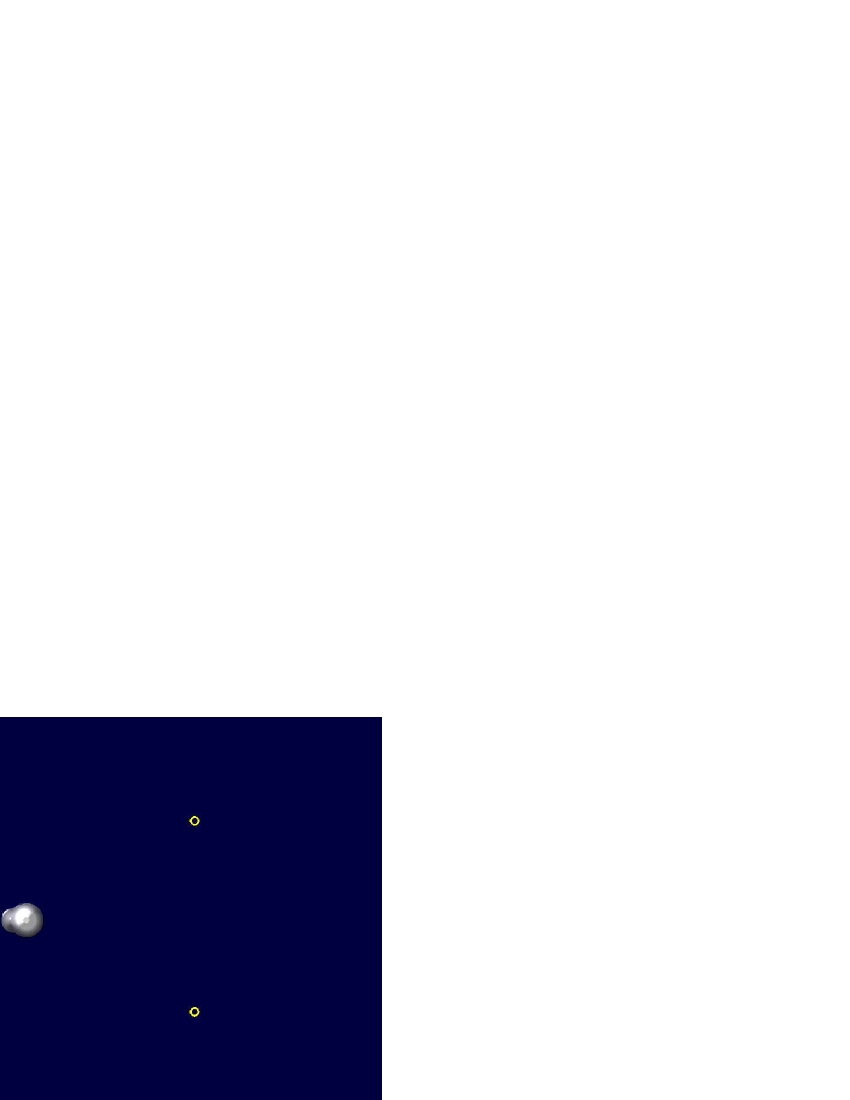
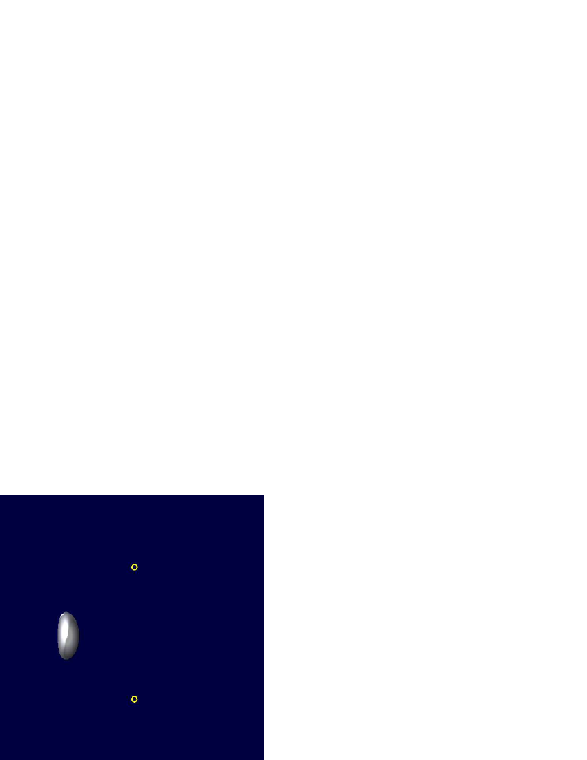
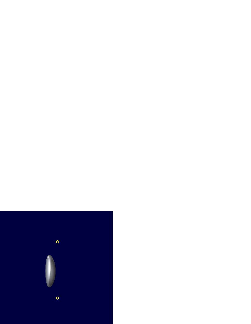
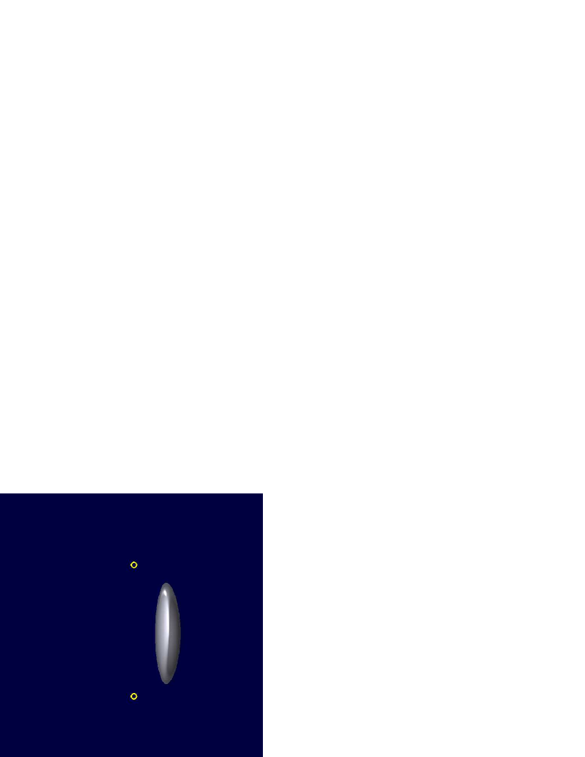
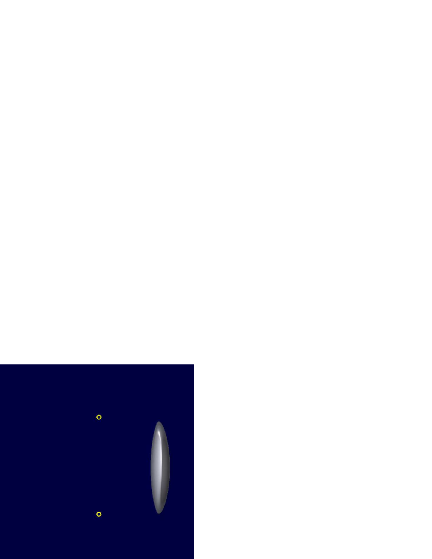
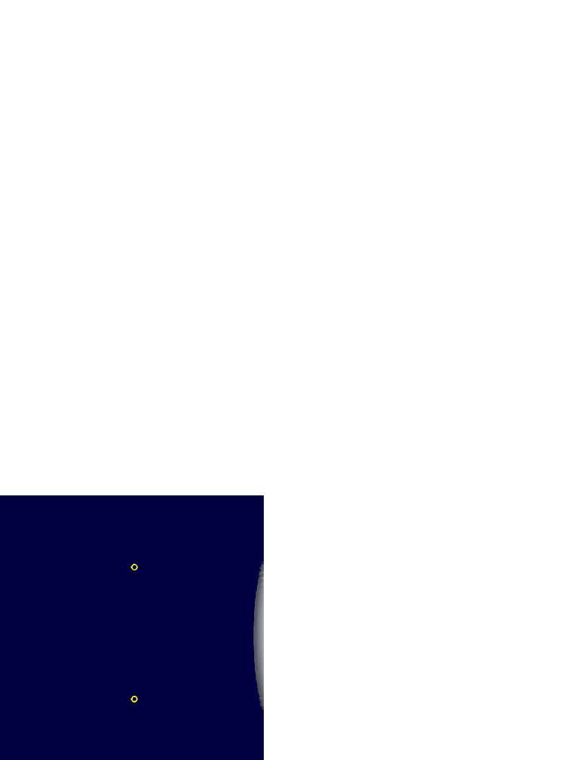
Figure 7: Six stages of the motion of the wave packet between two infinite parallel solenoids. Small yellow circles represent the positions and the sizes of the solenoids. The animation can be accessed on-line [19].

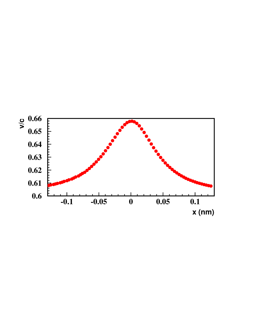
Figure 8: The velocity, as a function of position, of a wave packet moving along a straight line between two infinite parallel solenoids normalized to the speed of light . The solenoids are positioned at x=0.

5 The dynamics of the charged particle under the conditions of the Aharonov-Bohm effect

The controversy in the previous section, resulting from the solution of the Dirac equation, can be understood if we look again at the basic principles of classical mechanics.

The motion of a particle in the absence of a force in classical dynamics is obtained by solving the differential equation

$${d\vec{p}\over dt}=0,$$ (13)

where $\vec{p}=m\vec{v}$ is the momentum of a particle. The solution of this equation results in a constant velocity of the particle. The solution of the Dirac equation shows that, even if the force acting on the particle is zero, the velocity of the particle changes. To resolve the discrepancy between classical dynamics and the Dirac equation we need to look at the basics of how the Dirac equation of an electron is obtained.

In obtaining the Dirac equation from classical dynamics, the classical momentum $\vec{p}$ becomes a momentum operator $\hat{p}=-i\hbar\vec{\nabla}$. If the electron is in a given external field the momentum operator is replaced by $\hat{p}\rightarrow-i\hbar\vec{\nabla}+|e|\vec{A}$, where $e$ is the charge of the electron [20]. This replacement not only is not self-evident, but must be done in the first order equations [20]. Going backward from the Dirac equation into classical dynamics, one replaces the classical momentum $\vec{p}\rightarrow\vec{p}+|e|\vec{A}$. In the Lagrangian mechanics, the momentum $\vec{p}=m\vec{v}+|e|\vec{A}$ is called the generalized or canonical momentum [21]. By proper use of momentum conservation [21], the motion of an electron in the absence of a classical force can now be obtained by solving the differential equation

$${d{(\vec{p}+|e|\vec{A})}\over dt}=0.$$ (14)

Since $A_{x}$ does not explicitly depend on time, for the motion along the x-axis, Eq. (14) can be written as

$${dp_{x}\over dt}=-|e|{dA_{x}\over dt}=-|e|{dA_{x}\over dx}{dx\over dt}=-|e|{dA_{x}\over dx}v_{x}$$ (15)

In the relativistic case

$${dp_{x}\over dt}=\left(1-{v_{x}^{2}\over c^{2}}\right)^{-{3\over 2}}m_{0}{dv_{x}\over dt}.$$ (16)

Here $m_{0}$ is the rest mass of the electron. Using Eqs. (14) and (16) we get the differential equation for the velocity of the electron

$${dv_{x}\over dt}=-{|e|\over m_{0}}v_{x}\left(1-{v_{x}^{2}\over c^{2}}\right)^{3\over 2}{dA_{x}\over dx}.$$ (17)

Due to the relativistic motion, in the system of the solenoids the velocity differential $dv_{x}$ has to be substituted with $dv_{x}/(1-v_{x}^{2}/c^{2})$. This leads to the final form of the differential equation

$${dv_{x}\over dt}=-{|e|\over m_{0}}v_{x}\left(1-{v_{x}^{2}\over c^{2}}\right)^{5\over 2}{dA_{x}\over dx}.$$ (18)

Substituting $A_{x}$ from the Eq. (12) for $z=0$, electron motion along the mid-path between two solenoids, the differential equation for the velocity of the electron becomes

$${dv_{x}\over dt}={{2|e|\Phi}\over{\pi m_{0}}}{x\over{(x^{2}+a^{2})^{2}}}v_{x}\left(1-{v_{x}^{2}\over c^{2}}\right)^{5\over 2},$$ (19)

where $a$ is half the distance between two parallel infinite solenoids. This differential equation can be solved numerically.

Figure 9 shows a nearly perfect match between the solution of Eq. (19) and the solution of the Dirac equation. A small difference, a fraction of a percent, is the result of the numerical precision and the fact that in classical dynamics we calcute propagation of a particle, not a wave packet, therefore having no contribution of the localization to the initial condition.

In a little digression from the main point of this paper, we can show that the above application of the conservation of generalized or canonical momentum is not an exception. One can easily show that for the translationally invariant gauges, Eqs. (9) and (10), the conservation of generalized or canonical momentum is equivalent to the Lorentz force. Without changing the general result, for ease of calculation, we assume that the electric field $\vec{E}=0$ and the vector potential $\vec{A}$ is time independent.

The conservation of generalized or canonical momentum, Eq. (14), for the dynamics of an electron in a uniform magnetic field defined by the translationally invariant gauges, can now be rewritten as

$${d{\vec{p}}\over dt} = -|e|{d{\vec{A}}\over dt}=-|e|(\vec{v}\vec{\nabla})\vec{A}=-|e|(\vec{v}\vec{\nabla})(-B_{0}z\;\vec{i}+B_{0}x\;\vec{k})$$ (20)

$$= -|e|(-B_{0}v_{z}\;\vec{i}+B_{0}v_{x}\;\vec{k})=-|e|(\vec{v}\times\vec{B})$$

Eq. (20) shows that the Lorentz force is just a consequence of generalized or canonical momentum conservation. While not in such an explicit form, similar results were obtained by Semon and Taylor [21].

In a somewhat different way the same can be shown for the rotationally invariant gauge, Eq. (8). In this case we use conservation of the canonical angular momentum

$${d{(\vec{r}\times\vec{p}+|e|\;\vec{r}\times\vec{A})}\over dt}={d{(\vec{l}+|e|\;\vec{r}\times\vec{A})}\over dt}=0.$$ (21)

$\vec{l}=\vec{r}\times\vec{p}$ represents classical angular momentum. Eq. (21) can be rewritten as

$${d\vec{l}\over dt} = -|e|{d{(\vec{r}\times\vec{A})}\over dt}=-|e|\left({d\vec{r}\over dt}\times\vec{A}+\vec{r}\times{d\vec{A}\over dt}\right)$$ (22)

$$= -|e|\left(\vec{v}\times\vec{A}+\vec{r}\times(\vec{v}\vec{\nabla})\vec{A}\right)$$

Repeating the same algebra, but using the rotationally invariant gauge of the vector potential $\vec{A}$ , we get

$${d\vec{l}\over dt}=-|e|\;\vec{r}\times(\vec{v}\times\vec{B})=\vec{r}\times\vec{F}.$$ (23)

$\vec{F}$ is again the Lorentz force. With this we have shown the equivalence of the conservation of generalized or canonical momentum and canonical angular momentum, and the action of Lorentz force for all vector potential gauges of the uniform magnetic field.

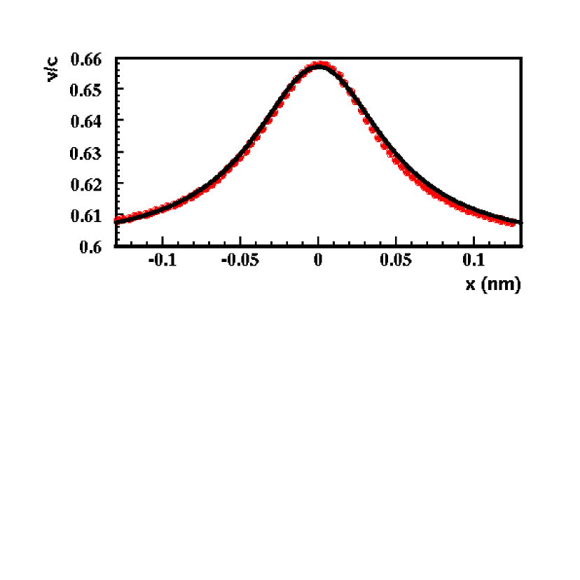
Figure 9: The velocity, as a function of position, of a wave packet moving along a straight line between two solenoids normalized to the speed of light. The circles represent the solution of the Dirac equation and the line represents the solution of Eq. (19) under the same conditions. The solenoids are positioned at x=0.

To conclude this section, we can look at the ongoing question if the Aharonov-Bohm effect is the result of a force changing the velocity of a particle passing on opposite sides of a single infinitely long solenoid, or there is only a quantum-mechanical phase shift [22, 23, 24, 25, 26, 27]. Quantum-mechanically such a question does not exist. The dynamics of the relativistic electron should be obtained only as a solution of the time-dependent Dirac equation. The solution of the Dirac equation shows that the velocity of a wave packet changes even in the region where the magnetic field is zero. Since the change of the velocity depends on the gradient of the vector potential, the velocity of the wave packet passing on the opposite sides of the solenoid will be different. Giving to the solution of the Dirac equation a classical picture, the requirement of the conservation of the canonical momentum in the region where the magnetic field is zero but the vector potential is not zero, also results in a velocity change of a charged particle. No mechanical forces need to be present in order for the velocity of the particle to change. From both, the solution of the Dirac equation and from the equivalence of the conservation of canonical momentum and the action of the Lorentz-force, one can also see that no work was done on the particle. The particle exits with the same energy regardless on which side of the solenoid it passed.

From the studies presented in this paper, the classical picture of the Aharonov-Bohm effect consists of the phase shift in the wave function of the particles passing on opposite sides of a solenoid being attributed to time lag resulting from different evolution of the velocities of the particles, without any involvement of mechanical forces and any change in energy. A phase shift then results in an interference pattern.

6 Conclusion

In conclusion, the full three-dimensional Finite Difference Time Domain (FDTD) method was developed to solve the Dirac equation. In this paper, the method was applied to the dynamics of the electron wave packet in a vector potential in the arrangements associated with the Aharonov-Bohm effect. The solution of the Dirac equation showed that the velocity of the electron wave packet changed even in the region where the electric and the magnetic fields were zero, and therefore no force acted on the electron.

The solution of the Dirac equation agreed with the prediction of classical dynamics under the assumption that the dynamics were defined by the conservation of generalized or canonical momentum. It was shown that in the case of a uniform magnetic field, the conservation of generalized or canonical momentum was equivalent to the action of the Lorentz force.

The studies in this paper have helped to establish a classical picture of the Aharonov-Bohm effect as the interference pattern resulting from the phase shift in the wave function of the particles passing on opposite sides of a solenoid attributed to a time lag resulting from different evolution of the velocities of the particles. No mechanical forces need to be involved and no change in energy of the particle occurs.

References

References

- [1] Simicevic N 2008 arXiv:0812.1807v1 [physics.comp-ph]
- [2] Simicevic N 2009 arXiv:0901.3765v1 [quant-ph]
- [3] Yee K S 1966 IEEE Trans. Antennas Propagat. AP-14 302
- [4] Klein O 1929 Z. Phys. 53 157
- [5] Aharonov Y and Bohm D 1959 Phys. Rev. 115 485
- [6] Chambers R G 1960 Phys. Rev. Lett. 5 3
- [7] Tonomura A, Osakabe N, Matsuda T, Kawasaki T, Endo J, Yano S, and Yamada H 1986 Phys. Rev. Lett. 56 792
- [8] Osakabe N, Matsuda T, Kawasaki T, Endo J, Tonomura A, Yano S, and Yamada H Phys. Rev. A 34 815
- [9] Peshkin M and Tonomura A 1989 The Aharonov-Bohm effect (Lecture Notes in Physics vol 340) (Berlin: Springer).
- [10] Hegerfeldt G C and Neuman J T 2008 J. Phys. A: Math. Theor. 41 155305
- [11] Boyer T H 2006 J. Phys. A: Math. Gen. 39 3455
- [12] Boyer T H 2008 Found. Phys. 38 498
- [13] Caprez A, Barwick B, and Batelaan H 2007 Phys. Rev. Lett. 99 210401
- [14] Greiner W, Muller B, and Rafelski J 1985 Quantum Electrodynamics of Strong Fields(Berlin: Springer-Verlag).
- [15] Sakurai J J 1987 Advanced Quantum Mechanics (Redwood City: Addison-Wesley).
- [16] Huang K 1952 Am. J. Phys. 20 479
- [17] Schliemann J 2008 Phys. Rev. B 77 125303
- [18] Demikhovskii V Ya, Maksimova G M, and Frolova E V 2008 Phys. Rev. B 78 115401
- [19] Simicevic N 2008 http://caps.phys.latech.edu/neven/ab/
- [20] Beresteckii V B, Lifshitz E M, and Pitaevskii L P 1982 Quantum Electrodynamics (Oxford: Butterworth Heinemann).
- [21] Semon M D and Taylor J R 1996 Am. J. Phys. 64 1361
- [22] Zhu X and Henneberger C 1990 J. Phys. A: Math. Gen. 23 3983
- [23] Shelenkov A L 1998 Europhys. Lett. 43 623
- [24] Keating J P and Robbins J M 2001 J. Phys. A: Math. Gen. 34 807
- [25] Gronniger G, Simmons Z, Gilbert S, Caprez A, and Batelaan H 2006, (preprint)
- [26] Horsley S A R and Babiker M 2005 Phys. Rev. Lett.95 010405
- [27] Horsley S A R and Babiker M 2007 J. Phys. B: At. Mol. Opt. Phys. 40 2003