Field theoretical approach to the description of the coherent structures in $2D$ fluids and plasmas

Abstract

Evolving from turbulent states the $2D$ fluids and the plasmas reach states characterized by a high degree of order, consisting of few vortices. These asymptotic states represent a small subset in the space of functions and are characterised by properties that are difficult to identify in a direct approach. The field theoretical approach to the dynamics and to the asymptotic states of fluids and plasmas in $2D$ provides a considerable extension of the usual perspective. The present works discusses a series of consequences of the field theoretical approach, when it is applied to particular problems. The discussion is developed around known physical problems: the current density profiles in cylindrical plasma, the density pinch in tokamak and the concentration of vorticity.

1 Introduction

The fluids and plasma exhibit in two-dimensions a strong tendency to self-organisation in the undriven evolution towards stationary states. As shown by experiments and numerical simulation, the $2D$ fluids and plasmas reach states of high coherency of the flow, generated by concentration of vorticity in few large scale vortical flows. The process is essentially non-dissipative since the energy is almost conserved during this process. The presence of dissipation is however essential since breaking up of streamlines and reconnection into larger structures is only possible in the presence of irreversible resistive-like mechanisms. The vortex merging is the typical process and a large number of studies have been done both experimentally and by numerical simulation. When the initial state is turbulent one may invoke arguments related with the inverse cascade of energy in $2D$ but this approach has limitted relevance when the process has evolved to the point where the number of cuasi-coherent structures is large: the high number of irreducible correlations necessary to describe a statistical ensemble of turbulence with embedded structures invalidates any perturbative considerations.

The problem of evolution towards the asymptotic coherent flow states is very complex and possibly different approaches must be developed to examine different aspects of it. For the states close to the final, organised one, the field theoretical formulation seems adequate. This is confirmed by the purely analytic derivation of the sinh-Poisson equation (describing the asymptotic states of the Euler fluid) and by the derivation of a new equation, for plasma and planetary atmosphere vortices, with substantial practical confirmation.

The particular nature of the physical systems that are investigated is reflected in construction of the Lagrangian of the field theoretical model: for point-like vortices we have to adopt an algebraic formulation of the fields, namely $su\left(2\right)$. For short range interaction we need the Higgs mechanism to generate a mass for the photon, and this imposes a particular form for the scalar matter self-interaction. Finally, in particular cases it appears possible that the $su\left(2\right)$ structure is reduced to the Abelian substructure (this is possibly similar to the Abelian dominance) and the nature of the extrema of the action functional changes significantly.

In the present work we apply the results of the models developed before. Since these models lead to equations describing the stationary states (flows) of lowest energy of the physical systems, the application should consists basically in solving these equations and confronting with experiments or observations. However some of these equations are already known and eventually they have been derived from different considerations, like the statistical theory. We will make a comparison between our approach and the statistical one.

The following partial conclusions seem to be supported by the analysis of the applications that are presented below.

1. the field theoretical model of the current profiles in tokamak is compatible with the Liouville equation. Comparison with the model of J. B. Taylor gives interesting suggestions for the physical interpretation of the FT parameters.

2. for the Euler fluid we obtain in FT a possible confirmation of the existence of a current of vorticity leading to concentration into filaments.

3. for the $2D$ plasma in strong magnetic field we obtain patterns of vortical flows that confirm previous numerical calculations.

4. for the LH transtion, we obtain, after a renormalisation of the Larmor radius into an effective Larmor radius, profiles of electric fields at the edge (in H mode) that are compatible with the experiments

5. for the density pinch we are able to build a physical picture that is consistent with the idea that the pinch of density is due to a pinch of vorticity.

6. for the $2D$ atmosphere we obtain quantitative results that compares (very) well with the observations of tropical cyclone.

7. for the Abelian dominance model the first results show the existence of ring-type vortices.

The various physically relevant cases are included in the following classification

Current $J$ Abelian	$\Delta\psi+\exp\left(\psi\right)=0$	conformal invariant	no $\rho_{s}$
Euler Non-Abelian	$\Delta\psi+\sinh\psi=0$	conformal invariant	no $\rho_{s}$
Superfluid Abelian	$\Delta\psi=\exp\left(\psi\right)-1$	n.a. (Minardi?)	finite $\rho_{s}$
CHM Non-Abelian	$\Delta\psi=\pm\sinh\psi\left(\cosh\psi-1\right)$	non-topological	finite $\rho_{s}$
CHM Abelian	$\Delta\psi=e^{\psi}\left(e^{\psi}-1\right)$	topological	finite $\rho_{s}$

2 The Liouville equation

2.1 Applications of the Liouville equation

There are at least three physical problems that may imply a description in terms of the Liouville equation:

1. the natural current profile in tokamak plasma

2. the snake of density in JET and other tokamaks

3. the filament of current density developed on a particular magnetic surface in tokamak (see Huysmans)

The last two phenomena seem to result from a concentration of a scalar field (density and respectively the current density) and show robustness. The last property is an indication that the system has reached an equilibrium that is of a purely nonlinear nature, analogous to the relaxed states, therefore they could be derived from the extremum of an action functional.

2.1.1 The current profile

The statistical theory of J.B. Taylor (and also : Montgomery, etc.) relies on the principle of maximum entropy, keeping the total energy and the total number of particles constant. It leads to the Liouville equation.

The constant entropy principle used by Minardi leads to the equation for the current and is well verified by statistical analysis of the peaking factors for current, density, pressure.

The statistical studies carried out on a large set of discharges with the purpose of testing the prediction of the Turbulent Equipartition theory have suggested that the current density is given by the equation $\Delta j+\left(\lambda^{2}/4\right)j=0$ where $\lambda$ is a constant. Replacing $j=\Delta\psi$ and assuming that two space integrations are possible without introducing new physical effects, we would have the equation

$$\Delta\psi+\frac{\lambda^{2}}{4}\psi=0$$

that can be seen as a small $\psi$ approximation to

$$\Delta\psi+\frac{\lambda^{2}}{4}\left[\exp\left(\psi\right)-1\right]=0$$

We just note that this equation is of a similar form as

$$\Delta\chi=\exp\left(\chi\right)-1$$

that describes the superfluid streamfunction in the Abelian-Higgs model. Actually these equations are not compatible, except when taking the Lagrangian multiplier $\lambda^{2}/4$ negative. This suggests that the principle of constant entropy used by Minardi cannot be derived from the topological theory of vortices in superfluids.

We will examine below the Taylor approach to the natural current profile in tokamak.

2.1.2 The snake of density

The snake phenomenon has been observed in JET during the experiments of pellet injection and consisted in formation of persistent density perturbations at rational-$q$ surfaces. These structures persist over several sawtooth collapses and are difficult to explain as magnetic perturbations. On the other hand there are indications that the tokamak plasma density has an anomalous radial pinch, much larger than that of the neoclassical origin. Apparently in the class of phenomena one should also include the persistent impurity accumulation in laser blow-off injected impurity, observed in experiments in TCV. There are several studies of the statistical properties of the correlations between the peaking factors for density, current density or pressure, with plasma parameters and these studies seem to support the idea of turbulent equipartition of the theromodynamic invariants. However we should note that these studies involve quantities expressed as global variables (like averages) and they can hide other dependences not immediately obvious.

We consider the possibility that the particle density behavior (and particularly the snake phenomenon) can be connected with the existence of attracting solutions of certain nonlinear integrable equations.

The reason to consider the sinh-Poisson equation comes from the existing proofs that this equation governs the asymptotic states of ideal fluids, or, more generally, of $2D$ systems that can be reduced to the dynamics of point-like elements interacting by the potential which is the inverse of the Laplacean operator (Jackiw and Pi, Spineanu and Vlad). This equation is however obtained when there are two kinds of elements (like positive and negative vorticity) and they are of equal number, $n_{+}=n_{-}$. Then the sinh-Poisson equation is obtained as governing the states with maximum entropy of the discrete statistical system at negative temperature (Montgomery et al.). Since the equation for the current density mentioned above is derived under the assumption of turbulent equipartition, the two descriptions may be related. However, the solutions for the unbalanced system of elements, $\alpha\equiv n_{+}/n_{-}\neq 1$, $\Delta\phi=\left(\lambda^{2}/8\right)\left[\exp\left(\phi\right)/\sqrt{\alpha}-\sqrt{\alpha}\exp\left(-\phi\right)\right]$ have been obtained numerically (Pointin and Lundgren) and have been shown to have higher entropy and higher stability than those of the sinh-Poisson, precisely the characteristics we are seeking for. The limiting form of the unbalanced equation is the Liouville equation, $\Delta\phi=\left(\lambda^{2}/8\right)\exp\left(-\phi\right)$.

3 Classical physical interpretation of natural current profile in tokamak

The model is simplified in order to exhibit the essential aspect of current self-organization in tokamak. The equation is

$$\mathbf{\nabla\times}\left(\mathbf{J\times B}\right)=0$$

or

$$B_{0}\frac{\partial J}{\partial z}+\left(\mathbf{B}_{\perp}\cdot\mathbf{\nabla}_{\perp}\right)J\mathbf{=}0$$

with

$$\mathbf{B}_{\perp} = -\mathbf{\nabla}\psi\times\widehat{\mathbf{n}}$$

$$J \equiv J_{z}=\nabla_{\perp}^{2}\psi$$

In the work of J.B. Taylor (1993) it is shown that a reasonable assumption is that the current density should consists of filaments, acted upon by $\mathbf{B}_{\perp}$ as a velocity field and with $z$ as time. The position of a filament is $\mathbf{r}_{i}\left(z\right)\equiv\left[x_{i}\left(z\right),y_{i}\left(z\right)\right]$ and the equations of motion are (all filaments are assumed equal $j_{0}$)

$$j_{0}\frac{dx_{i}}{dz} = \frac{1}{B_{0}}\frac{\partial H}{\partial y_{i}}$$

$$j_{0}\frac{dy_{i}}{dz} = -\frac{1}{B_{0}}\frac{\partial H}{\partial x_{i}}$$

where

$$H = \sum\limits_{k<i}j_{0}^{2}U\left(\mathbf{r}_{i},\mathbf{r}_{k}\right)$$

$$\mathbf{\nabla}_{\perp}^{2}U\left(\mathbf{r},\mathbf{r}^{{}^{\prime}}\right) = \delta\left(\mathbf{r-r}^{{}^{\prime}}\right)$$

In an infinite region, the Green function $U\left(\mathbf{r,r}^{{}^{\prime}}\right)$ of the Laplace operator is

$$U\left(\mathbf{r,r}^{{}^{\prime}}\right)=\ln\left|\mathbf{r-r}^{{}^{\prime}}\right|$$

The current distribution and the magnetic flux function $\psi$ (streamfunction)

$$J = \sum\limits_{i}j_{0}\delta\left(\mathbf{r-r}_{i}\right)$$ (1)

$$\psi = j_{0}\sum\limits_{i}U\left(\mathbf{r,r}_{i}\right)$$

The statistical description of the system.

The energy of the system is $H$ and it is strictly conserved and a microcanonical ensemble, where the joint probability distribution of the positions of $N$ filaments is

$$\rho\left(\left\{\mathbf{r}_{i}\right\}\right)\sim\delta\left(E-H\left\{\mathbf{r}_{i}\right\}\right)$$

is appropriate. The entropy

$$S=-k\int d\mathbf{r}\ n\left(\mathbf{r}\right)\ln\left[n\left(\mathbf{r}\right)\right]$$

is a measure of the number of microscopic configurations corresponding to a macroscopic configuration $n\left(\mathbf{r}\right)$.

Statistical equilibrium is obtained by maximizing $S$ (the entropy) under the constraint of energy conservation and fixed total number of filaments

$$E\ \text{(fixed)} = j_{0}\int d\mathbf{r}\ n\left(\mathbf{r}\right)\psi\left(\mathbf{r}\right)$$

$$N\ \text{(fixed)} = \int d\mathbf{r}\ n\left(\mathbf{r}\right)$$

The continuum version of the magnetic flux function ($z$-component of the magnetic potential), $\psi$ is obtained from Eq.(1)

$$\psi\left(\mathbf{r}\right)=j_{0}\int d\mathbf{r}^{{}^{\prime}}\ U\left(\mathbf{r,r}^{{}^{\prime}}\right)n\left(\mathbf{r}^{{}^{\prime}}\right)$$

The equilibrium current distribution obtained by extremizing

$$S-\beta E-\gamma N$$

is

$$J\left(\mathbf{r}\right) = j_{0}\left\langle n\left(\mathbf{r}\right)\right\rangle$$

$$= K\exp\left[-\beta j_{0}\psi\left(\mathbf{r}\right)\right]$$

Natural current density profiles. Take $\psi$ to be zero on the magnetic axis. Then

$$\nabla_{\perp}^{2}\psi=J_{0}\exp\left(-\lambda\psi\right)$$

For circular symmetry in a tokamak of radius $a$,

$$\psi\left(r\right)=\frac{2}{\lambda}\ln\left(1+\alpha\frac{r^{2}}{a^{2}}\right)$$

where

$$\alpha=J_{0}\lambda\frac{a^{2}}{8\pi}$$

Introducing the total current $I$,

$$I=Nj_{0}$$

it is found a relation between the peaking factor of the current density, $\alpha$ , and the inverse temperature $\beta$ of the current filaments

$$\beta Nj_{0}^{2}=\frac{8\pi\alpha}{1+\alpha}$$

Uniform current (which means that the whole plasma volume is chaotic) is obtained for a magnetic temperature $T_{m}\equiv 1/\beta$ of

$$\alpha=0\ \text{or}\ T_{m}\rightarrow\infty$$

and it is identified a critical magnetic temperature $T_{m}^{c}$ where the totality of the current is concentrated into a singular central filament,

$$\alpha\rightarrow\infty\ \text{or}\ T_{m}\rightarrow T_{m}^{c}\equiv\frac{Nj_{0}^{2}}{8\pi}$$

Values of the magnetic temperatures between $0$ and $T_{m}^{c}$ are not accessible.

Hollow current profiles correspond to negative magnetic temperatures. They are only accessible through the infinite value of the magnetic temperature, $T_{m}\rightarrow\infty$, which in terms of profiles means that the current passes first through a state of uniform distribution.

To compare with Field Theory we take the two equations

$$\text{FT:}\ \Delta\ln\rho=\pm\frac{2e^{2}}{c\kappa}\rho$$

This is the Liouville equation after the substitution

$$\rho=\exp\left(\psi\right)$$

It has nonsingular and non-negative solutions for $\rho$ when it has the form

$$\Delta\ln\rho+\left|\gamma\right|\rho=0$$

Then the convention on the choice of signs in the right hand side follows from the choice of sign for $\kappa$:

1. when $\kappa=\left|\kappa\right|>0$ one has to take the $-$ sign in the right hand side, such that

   $$\Delta\ln\rho=-\frac{2e^{2}}{c\left|\kappa\right|}\rho$$

   or

   $$\Delta\psi+\left(\frac{2e^{2}}{c\kappa}\right)\exp\left(\psi\right)=0$$

2. when $\kappa=-\left|\kappa\right|<0$ one has to take the $+$ sign in the right hand side, such that

   $$\Delta\ln\rho=+\frac{2e^{2}}{c\kappa}\rho=-\frac{2e^{2}}{c\left|\kappa\right|}\rho$$

   or

   $$\Delta\psi+\left(\frac{2e^{2}}{c\left|\kappa\right|}\right)\exp\left(\psi\right)=0$$

Therefore the equation is always the same, whatever is the sign in front of the Chern-Simons term.

In Taylor’s theory, we have

$$\mathbf{\nabla}_{\perp}^{2}\psi=J_{0}\exp\left(-\lambda\psi\right)$$

with

$$\lambda = \frac{8\pi\alpha}{J_{0}a^{2}}$$

$$\frac{8\pi\alpha}{1+\alpha} = \frac{1}{T_{m}}Nj_{0}^{2}$$

We change the variable

$$\psi\rightarrow\psi^{{}^{\prime}}=-\lambda\psi$$

and the Taylor’s equation becomes

$$\left(-\lambda\right)\mathbf{\nabla}_{\perp}^{2}\psi^{{}^{\prime}} = J_{0}\exp\left(\psi^{{}^{\prime}}\right)$$

$$\mathbf{\nabla}_{\perp}^{2}\psi^{{}^{\prime}}+\left(\frac{J_{0}}{\lambda}\right)\exp\left(\psi^{{}^{\prime}}\right) = 0$$

or

$$\frac{J_{0}}{\lambda}=\frac{J_{0}^{2}a^{2}}{8\pi\alpha}=\frac{2e^{2}}{c\left|\kappa\right|}$$

Then we can translate the results obtained by Taylor:

1. when the peaking factor $\alpha$ goes to $0$, (i.e. the magnetic temperature $T_{m}\rightarrow\infty$) the current profile is fully relaxed to a uniform distribution; This corresponds of vanishing $\kappa$ in the field theory: no Chern-Simons is present.

2. when the peaking factor $\alpha$ goes to $\infty$, (i.e. the magnetic temperature reaches the critical value, $T_{m}\rightarrow T_{m}^{c}$) the current is strongly concentrated on the axis. This corresponds to infinite value for $\kappa$ in the field theory, $\left|\kappa\right|\rightarrow\infty$: the Chern-Simons term is largely dominating everything else in the Lagrangian.

3. Negative magnetic temperature

   $$T_{m}<0$$

   are obtained in the Taylor’s model when

   $$\alpha<0$$

   or, the current profile is hollow. In field theory this corresponds to a change of sign of $\kappa$. But the equation remains the same. The field theory starts with a certain sign of $\kappa$, then the Chern-Simons term is suppressed (taking $\left|\kappa\right|\rightarrow 0$) (leading to uniform solution for $\psi\rightarrow-\infty$ everywhere, while $\Delta\psi$ may remain finite). After that the CS term is re-established but with an effect which is opposite to the previous regime.

Everything should be seen as an evolution on the manifold of SELF-DUAL states, or solutions of the Liouville equation. The parameter that moves the states on this manifold is $\kappa$.

The following quantities have dimension of inverse distance squared

$$\frac{J_{0}}{\lambda}=\frac{2e^{2}}{c\left|\kappa\right|}=\frac{1}{\rho^{2}}$$

where $\rho$ is a distance. This distance will be the natural unit of space-like quantities in the problem. For example if our physical problem is localised spatially in the disk of radius $a$, the adimensional space range is

$$L\equiv\frac{a}{\rho}$$

We note that the space unit $\rho$ is proportional with $\kappa$. We can say that the passage of the system from a concentrated current profile to a hollow current profile includes a state of strong localisation, where the natural space unit is extremely small, which means that different parts of the system are separated and non-interacting (physically this means chaos and uniform current everywhere).

4 The equation for the velocity of the fluid of point-like vortices in static configurations

In the field theoretical models of developed for the $2D$ current density distribution and for the vorticity in ring-type structures in fluids or plasmas, it is found that the magnetic potential (that carries the interaction between the point-like vortices) has spatial components given by the equations:

$$\mathbf{A}=\nabla\theta\pm\Lambda\nabla\times\ln\rho$$

where $c$ is a dimensional constant (in the quantum theroies where the objective is to describe the Abrikosov Nielsen Olesen vortices, $\Lambda\equiv\hbar c/\left(2e\right)$).

We want to calculate the contribution of the physical velocity in the balance equation at stationarity

$$\left(\mathbf{v\cdot\nabla}\right)\mathbf{v=-\nabla}p$$

where $p$ is the scalar pressure in the fluid. The physical velocity is just the last term in the expression of the magnetic potential $\mathbf{A}$.

Using the definition of $\mathbf{v}$ we have

$$\left(\mathbf{v\cdot\nabla}\right)\mathbf{v=}\left[\left(\Lambda\nabla\times\ln\rho\right)\cdot\mathbf{\nabla}\right]\left(\Lambda\nabla\times\ln\rho\right)$$

or

$$\nabla\times\ln\rho\rightarrow\widehat{\mathbf{e}}_{z}\times\mathbf{\nabla}\left(\ln\rho\right)$$

We extract for the next calculations the physical coefficient $\Lambda$. This will leave some apparent incompatibilities in dimensions, but at the end $\Lambda$ should be re-introduced.

$$\left(\mathbf{v\cdot\nabla}\right)\mathbf{v}$$

$$= \left\{\left[\widehat{\mathbf{e}}_{z}\times\mathbf{\nabla}\left(\ln\rho\right)\right]\cdot\mathbf{\nabla}\right\}\left[\widehat{\mathbf{e}}_{z}\times\mathbf{\nabla}\left(\ln\rho\right)\right]$$

$$= \left[\varepsilon^{ik}\partial_{k}\left(\ln\rho\right)\right]\partial_{i}\left[\varepsilon^{jl}\partial_{l}\left(\ln\rho\right)\right]$$

$$= \varepsilon^{ik}\varepsilon^{jl}\partial_{k}\left(\ln\rho\right)\partial_{i}\partial_{l}\left(\ln\rho\right)$$

This is a vector and we have to calculate the two components in plane. For $j=x$,

$$\left[\left(\mathbf{v\cdot\nabla}\right)\mathbf{v}\right]_{x}$$

$$= \varepsilon^{xl}\left\{\varepsilon^{ik}\partial_{k}\left(\ln\rho\right)\partial_{i}\partial_{l}\left(\ln\rho\right)\right\}$$

$$= \varepsilon^{xy}\left\{\varepsilon^{ik}\partial_{k}\left(\ln\rho\right)\partial_{i}\partial_{y}\left(\ln\rho\right)\right\}$$

the summation over $l$ consists of just one term, $l=y$. We have considered the convention $\varepsilon^{xy}=1$. We make the summations over $i$ and $k$:

$$\left[\left(\mathbf{v\cdot\nabla}\right)\mathbf{v}\right]_{x}$$

$$= \varepsilon^{ik}\partial_{k}\left(\ln\rho\right)\partial_{i}\partial_{y}\left(\ln\rho\right)$$

$$= \varepsilon^{xy}\partial_{y}\left(\ln\rho\right)\partial_{x}\partial_{y}\left(\ln\rho\right)+\varepsilon^{yx}\partial_{x}\left(\ln\rho\right)\partial_{y}\partial_{y}\left(\ln\rho\right)$$

$$= \partial_{x}\left\{\frac{1}{2}\left[\partial_{y}\left(\ln\rho\right)\right]^{2}\right\}-\partial_{x}\left(\ln\rho\right)\partial_{y}^{2}\left(\ln\rho\right)$$

The other component, $j=y$

$$\left[\left(\mathbf{v\cdot\nabla}\right)\mathbf{v}\right]_{y}$$

$$= \varepsilon^{yl}\left\{\varepsilon^{ik}\partial_{k}\left(\ln\rho\right)\partial_{i}\partial_{l}\left(\ln\rho\right)\right\}$$

$$= \varepsilon^{yx}\left\{\varepsilon^{ik}\partial_{k}\left(\ln\rho\right)\partial_{i}\partial_{x}\left(\ln\rho\right)\right\}$$

$$= -\varepsilon^{ik}\partial_{k}\left(\ln\rho\right)\partial_{i}\partial_{x}\left(\ln\rho\right)$$

with the convention $\varepsilon^{yx}=-1$. Now we make the summation over $i$ and $k$:

$$\left[\left(\mathbf{v\cdot\nabla}\right)\mathbf{v}\right]_{y}$$

$$= -\varepsilon^{ik}\partial_{k}\left(\ln\rho\right)\partial_{i}\partial_{x}\left(\ln\rho\right)$$

$$= -\varepsilon^{xy}\partial_{y}\left(\ln\rho\right)\partial_{x}\partial_{x}\left(\ln\rho\right)-\varepsilon^{yx}\partial_{x}\left(\ln\rho\right)\partial_{y}\partial_{x}\left(\ln\rho\right)$$

$$= -\partial_{y}\left(\ln\rho\right)\partial_{x}^{2}\left(\ln\rho\right)+\partial_{y}\left\{\frac{1}{2}\left[\partial_{x}\left(\ln\rho\right)\right]^{2}\right\}$$

In the expression of the first component we take into account the differential equation verified by $\rho$

$$\Delta\ln\rho=\alpha\rho$$

where $\alpha$ is a constant. Then

$$\partial_{x}^{2}\left(\ln\rho\right)+\partial_{y}^{2}\left(\ln\rho\right)=\alpha\rho$$

and replace

$$\partial_{y}^{2}\left(\ln\rho\right)=\alpha\rho-\partial_{x}^{2}\left(\ln\rho\right)$$

in the expression of the $x$ component

$$\left[\left(\mathbf{v\cdot\nabla}\right)\mathbf{v}\right]_{x}$$

$$= \partial_{x}\left\{\frac{1}{2}\left[\partial_{y}\left(\ln\rho\right)\right]^{2}\right\}-\partial_{x}\left(\ln\rho\right)\partial_{y}^{2}\left(\ln\rho\right)$$

$$= \partial_{x}\left\{\frac{1}{2}\left[\partial_{y}\left(\ln\rho\right)\right]^{2}\right\}$$

$$-\partial_{x}\left(\ln\rho\right)\left[\alpha\rho-\partial_{x}^{2}\left(\ln\rho\right)\right]$$

$$= \partial_{x}\left\{\frac{1}{2}\left[\partial_{y}\left(\ln\rho\right)\right]^{2}\right\}$$

$$-\partial_{x}\left(\ln\rho\right)\alpha\rho$$

$$+\partial_{x}\left(\ln\rho\right)\partial_{x}^{2}\left(\ln\rho\right)$$

$$= \partial_{x}\left\{\frac{1}{2}\left[\partial_{y}\left(\ln\rho\right)\right]^{2}\right\}$$

$$-\left(\partial_{x}\rho\right)\alpha$$

$$+\partial_{x}\left\{\frac{1}{2}\left[\partial_{x}\left(\ln\rho\right)\right]^{2}\right\}$$

$$= \partial_{x}\Xi$$

where

$$\Xi \equiv \frac{1}{2}\left[\partial_{y}\left(\ln\rho\right)\right]^{2}+\frac{1}{2}\left[\partial_{x}\left(\ln\rho\right)\right]^{2}-\alpha\rho$$

$$= \frac{1}{2\rho^{2}}\left[\left(\partial_{x}\rho\right)^{2}+\left(\partial_{y}\rho\right)^{2}\right]-\alpha\rho$$

Another expression can be obtained if we substitute

$$\partial_{x}^{2}\left(\ln\rho\right) = \partial_{x}\left(\frac{\partial_{x}\rho}{\rho}\right)$$

$$= \frac{\partial_{x}^{2}\rho}{\rho}-\frac{\left(\partial_{x}\rho\right)^{2}}{\rho^{2}}$$

$$\frac{\left(\partial_{x}\rho\right)^{2}}{\rho^{2}}+\frac{\left(\partial_{y}\rho\right)^{2}}{\rho^{2}}$$

$$= \frac{\partial_{x}^{2}\rho}{\rho}-\partial_{x}^{2}\left(\ln\rho\right)+\frac{\partial_{y}^{2}\rho}{\rho}-\partial_{y}^{2}\left(\ln\rho\right)$$

$$= \frac{\Delta\rho}{\rho}-\Delta\left(\ln\rho\right)$$

$$= \frac{\Delta\rho}{\rho}-\alpha\rho$$

Then

$$\Xi = \frac{1}{2\rho^{2}}\left[\left(\partial_{x}\rho\right)^{2}+\left(\partial_{y}\rho\right)^{2}\right]-\alpha\rho$$

$$= \frac{1}{2}\left(\frac{\Delta\rho}{\rho}-\alpha\rho\right)-\alpha\rho$$

$$= \frac{1}{2}\frac{\Delta\rho}{\rho}-\frac{3}{2}\alpha\rho$$

In conclusion the $x$ component is

$$\left[\left(\mathbf{v\cdot\nabla}\right)\mathbf{v}\right]_{x}$$

$$= -\partial_{x}\left\{\frac{3}{2}\alpha\rho-\frac{1}{2}\frac{\Delta\rho}{\rho}\right\}$$

and the pressure is

$$p = \frac{3}{2}\alpha\rho-\frac{1}{2}\frac{\Delta\rho}{\rho}$$

$$= \frac{3}{2}\Delta\left(\ln\rho\right)-\frac{1}{2}\frac{\Delta\rho}{\rho}$$

If we take

$$\rho=\exp\psi$$

we have

$$\frac{\Delta\rho}{\rho} = \left(\mathbf{\nabla}\psi\right)^{2}+\Delta\psi$$

$$= v^{2}+\omega$$

and

$$p = \frac{3}{2}\omega-\frac{1}{2}\left(v^{2}+\omega\right)$$

$$= \omega-\frac{1}{2}v^{2}$$

where $\omega$ and $v$ are normalized.

This is the equivalent physical pressure that exists in a fluid for which the Liouville equation is fullfilled. We used the field theoretical formulation in order to calculate the pressure from the equation of momentum conservation, at stationarity.

NOTE

We remark that the quantity

$$-\frac{1}{2}v^{2}+\omega$$

looks similar to the square

$$\mathcal{A}^{\dagger}\mathcal{A}$$

where

$$\mathcal{A}_{\mu}\equiv A_{\mu}\pm\sqrt{\frac{\kappa}{2}}\phi$$

as a ” vector potential” of a flat curvature space.

5 The physical pressure for the EULER fluid

We take the part of the velocity that is determined by the gradient of the vorticity density. The balance equation at stationarity is

$$\left(\mathbf{v}^{\omega}\cdot\mathbf{\nabla}\right)\mathbf{v}^{\omega}\sim-\frac{1}{\rho_{0}}\mathbf{\nabla}p$$

and

$$\mathbf{v}^{\omega} \equiv \mathbf{\nabla}\omega=\mathbf{\nabla}\left(-\sinh\psi\right)$$

$$= -\cosh\psi\mathbf{\nabla}\psi$$

Then

$$\left(\mathbf{v}^{\omega}\cdot\mathbf{\nabla}\right)\mathbf{v}^{\omega}=\cosh\psi\left(\mathbf{\nabla}\psi\cdot\mathbf{\nabla}\right)\left(\cosh\psi\mathbf{\nabla}\psi\right)$$

$$\left(\partial_{i}\psi\right)\partial_{i}\left[\cosh\psi\left(\partial_{j}\psi\right)\right]$$

$$= \left(\partial_{i}\psi\right)\sinh\psi\left(\partial_{i}\psi\right)\left(\partial_{j}\psi\right)+\left(\partial_{i}\psi\right)\cosh\psi\left(\partial_{i}\partial_{j}\psi\right)$$

$$\left(\mathbf{v}^{\omega}\cdot\mathbf{\nabla}\right)\mathbf{v}^{\omega}|_{j} = \sinh\psi\cosh\psi\left(\partial_{i}\psi\right)^{2}\left(\partial_{j}\psi\right)+\left(\cosh\psi\right)^{2}\left(\partial_{i}\psi\right)\left(\partial_{i}\partial_{j}\psi\right)$$

$$= \cosh\psi\left(\mathbf{\nabla}\psi\right)\cdot\left[\sinh\psi\left(\mathbf{\nabla}\psi\right)\left(\partial_{j}\psi\right)+\cosh\psi\mathbf{\nabla}\left(\partial_{j}\psi\right)\right]$$

We use the formula

$$\left(\mathbf{v\cdot\nabla}\right)\mathbf{v=\nabla}\left(\frac{v^{2}}{2}\right)-\mathbf{v\times}\left(\mathbf{\nabla\times v}\right)$$

Then

$$\left(\mathbf{v}^{\omega}\cdot\mathbf{\nabla}\right)\mathbf{v}^{\omega} = \mathbf{\nabla}\left(\frac{v^{\omega 2}}{2}\right)-\mathbf{v}^{\omega}\mathbf{\times}\left(\mathbf{\nabla\times v}^{\omega}\right)$$

$$= \mathbf{\nabla}\left[\frac{\left(\mathbf{\nabla}\omega\right)^{2}}{2}\right]-\mathbf{\nabla}\omega\times\left(\mathbf{\nabla\times\nabla}\omega\right)$$

$$= \mathbf{\nabla}\left[\frac{\left(\mathbf{\nabla}\omega\right)^{2}}{2}\right]$$

$$= \frac{1}{2}\mathbf{\nabla}\left[\mathbf{\nabla}\left(\sinh\psi\right)\right]^{2}=\frac{1}{2}\mathbf{\nabla}\left[\cosh\psi\left(\mathbf{\nabla}\psi\right)\right]^{2}$$

$$= \frac{1}{2}\mathbf{\nabla}\left[\left(\cosh\psi\right)^{2}\left(\mathbf{\nabla}\psi\right)^{2}\right]$$

or

$$\left(\mathbf{v}^{\omega}\cdot\mathbf{\nabla}\right)\mathbf{v}^{\omega}=-\frac{1}{\rho_{0}}\mathbf{\nabla}p$$

for

$$-\frac{1}{\rho_{0}}\mathbf{\nabla}p\equiv\mathbf{\nabla}\left[\frac{\left(\mathbf{\nabla}\omega\right)^{2}}{2}\right]$$

Take

$$\rho_{0} = \rho_{1}+\rho_{2}$$

$$= 2\cosh\psi$$

Then

$$\mathbf{\nabla}p = -2\cosh\psi\mathbf{\nabla}\left[\frac{\left(\mathbf{\nabla}\omega\right)^{2}}{2}\right]$$

$$= \left(-2\cosh\psi\right)\frac{1}{2}\mathbf{\nabla}\left[\left(\cosh\psi\right)^{2}\left(\mathbf{\nabla}\psi\right)^{2}\right]$$

This should be expressed as a gradient of a scalar function.

In order that the expression above to be written as the gradient of a scalar function (pressure) we start from thesecond part of the velocity expressed as

$$v_{x}^{\omega} \sim \frac{\partial}{\partial x}\left(\rho_{1}-\rho_{2}\right)$$

$$v_{y}^{\omega} \sim \frac{\partial}{\partial y}\left(\rho_{1}-\rho_{2}\right)$$

A typical gradient along this velocity is

$$\mathbf{v}^{\omega}\cdot\mathbf{\nabla} = v_{x}^{\omega}\frac{\partial}{\partial x}+v_{y}^{\omega}\frac{\partial}{\partial y}$$

$$= \frac{\partial}{\partial x}\left(\rho_{1}-\rho_{2}\right)\frac{\partial}{\partial x}+\frac{\partial}{\partial y}\left(\rho_{1}-\rho_{2}\right)\frac{\partial}{\partial y}$$

This may be applied in particular on one of the components of this velocity

$$\left(\mathbf{v}^{\omega}\cdot\mathbf{\nabla}\right)v_{x}^{\omega} = \left[\frac{\partial}{\partial x}\left(\rho_{1}-\rho_{2}\right)\frac{\partial}{\partial x}+\frac{\partial}{\partial y}\left(\rho_{1}-\rho_{2}\right)\frac{\partial}{\partial y}\right]\frac{\partial}{\partial x}\left(\rho_{1}-\rho_{2}\right)$$

$$\sim \frac{\partial\omega}{\partial x}\frac{\partial^{2}\omega}{\partial x^{2}}+\frac{\partial\omega}{\partial y}\frac{\partial^{2}\omega}{\partial y\partial x}$$

$$= \frac{\partial}{\partial x}\left[\frac{1}{2}\left(\frac{\partial\omega}{\partial x}\right)^{2}+\frac{1}{2}\left(\frac{\partial\omega}{\partial y}\right)^{2}\right]$$

and

$$\left(\mathbf{v}^{\omega}\cdot\mathbf{\nabla}\right)v_{y}^{\omega} = \left[\frac{\partial}{\partial x}\left(\rho_{1}-\rho_{2}\right)\frac{\partial}{\partial x}+\frac{\partial}{\partial y}\left(\rho_{1}-\rho_{2}\right)\frac{\partial}{\partial y}\right]\frac{\partial}{\partial y}\left(\rho_{1}-\rho_{2}\right)$$

$$\sim \frac{\partial\omega}{\partial x}\frac{\partial^{2}\omega}{\partial x\partial y}+\frac{\partial\omega}{\partial y}\frac{\partial^{2}\omega}{\partial y^{2}}$$

$$= \frac{\partial}{\partial y}\left[\frac{1}{2}\left(\frac{\partial\omega}{\partial x}\right)^{2}+\frac{1}{2}\left(\frac{\partial\omega}{\partial y}\right)^{2}\right]$$

We can conclude that a certain quantity is suggested:

$$\left(\mathbf{v}^{\omega}\cdot\mathbf{\nabla}\right)\mathbf{v}^{\omega}\sim-\frac{1}{\rho_{0}}\mathbf{\nabla}p$$

with the pressure

$$p\sim-\left[\frac{1}{2}\left(\frac{\partial\omega}{\partial x}\right)^{2}+\frac{1}{2}\left(\frac{\partial\omega}{\partial y}\right)^{2}\right]$$

This pressure is negative, as expected. Since we are approximately at self-duality for the Euler fluid we have

$$p \sim -\left[\frac{1}{2}\left(\frac{\partial\omega}{\partial x}\right)^{2}+\frac{1}{2}\left(\frac{\partial\omega}{\partial y}\right)^{2}\right]$$

$$= -\frac{1}{2}\left(\cosh\psi\right)^{2}\left[\left(\frac{\partial\psi}{\partial x}\right)^{2}+\left(\frac{\partial\psi}{\partial y}\right)^{2}\right]$$

$$= -\frac{1}{2}\left(\cosh\psi\right)^{2}\left|\mathbf{\nabla}\psi\right|^{2}$$

We use the formulas

$$\left(\cosh\psi\right)^{2} = 1+\left(\sinh\psi\right)^{2}$$

$$= 1+\omega^{2}$$

and

$$\left|\mathbf{\nabla}\psi\right|^{2}=\mathbf{v}^{2}$$

Then

$$p \sim -\frac{1}{2}\left(\cosh\psi\right)^{2}\left|\mathbf{\nabla}\psi\right|^{2}$$

$$= -\frac{1}{2}\left(1+\omega^{2}\right)\mathbf{v}^{2}$$

$$= -\frac{1}{2}\mathbf{v}^{2}+\omega^{2}\mathbf{v}^{2}$$

This part of the pressure of the fluid of point-like vortices arises from the part of the velocity that comes from the gradient of the density of point-like vortices. The calculation is also valid in the case of the Charney-Hasegawa-Mima (CHM) fluids, i.e. plasma and planetary atmosphere. We see that the pressure is most negative there where $\omega$ is higher, i.e. at the center of the vortex. However, there $\mathbf{v}$ is zero. It appears that the pressure is most negative somewhere between the maximum $\mathbf{v}$ and the center (maximum of $\omega$). Since the variation of the $\omega$-velocity $v^{\omega}$ is governed by the force resulting from the gradient of the pressure and the pressure has a negative minimum somewhere between the radius of maximum azimuthal wind and the center, it results that the pressure gradient acts such as to push the ”matter” = vorticity toward this point. This is the reason for the creation of the cyclone eye.

6 The curvature and the Self-dual state for the Euler fluid

We take two variables identical with those which at SD give us the zero-curvature condition.

$$\mathcal{A}_{+} = A_{+}-\lambda\phi$$

$$\mathcal{A}_{-} = A_{-}+\lambda\phi^{\dagger}$$

where

$$\lambda\equiv\text{ real constant}$$

and calculate (cf. Eq.(59) and followings of Dunne)

$$K_{\pm}\equiv\partial_{\pm}\mathcal{A}_{\mp}-\partial_{\mp}\mathcal{A}_{\pm}+\left[\mathcal{A}_{\pm},\mathcal{A}_{\mp}\right]$$

From the definitions we have

$$\phi = \phi_{1}E_{+}+\phi_{2}E_{-}$$

$$\phi^{\dagger} = \phi_{1}^{\ast}E_{-}+\phi_{2}^{\ast}E_{+}$$

and

$$A_{+} = aH$$

$$A_{-} = -a^{\ast}H$$

then

$$\mathcal{A}_{+} = A_{+}-\lambda\phi$$

$$= aH-\lambda\left(\phi_{1}E_{+}+\phi_{2}E_{-}\right)$$

$$\mathcal{A}_{-} = A_{-}+\lambda\phi^{\dagger}$$

$$= -a^{\ast}H+\lambda\left(\phi_{1}^{\ast}E_{-}+\phi_{2}^{\ast}E_{+}\right)$$

6.0.1 The expression of the curvature $K_{+}$

Let us take the $+$ sign:

$$K_{+}=$$

$$= \partial_{+}\mathcal{A}_{-}-\partial_{-}\mathcal{A}_{+}+\left[\mathcal{A}_{+},\mathcal{A}_{-}\right]$$

$$= \partial_{+}\left(A_{-}+\lambda\phi^{\dagger}\right)-\partial_{-}\left(A_{+}-\lambda\phi\right)+\left[A_{+}-\lambda\phi,A_{-}+\lambda\phi^{\dagger}\right]$$

$$= \partial_{+}\left[-a^{\ast}H+\lambda\left(\phi_{1}^{\ast}E_{-}+\phi_{2}^{\ast}E_{+}\right)\right]$$

$$-\partial_{-}\left[aH-\lambda\left(\phi_{1}E_{+}+\phi_{2}E_{-}\right)\right]$$

$$+\left[aH-\lambda\left(\phi_{1}E_{+}+\phi_{2}E_{-}\right),-a^{\ast}H+\lambda\left(\phi_{1}^{\ast}E_{-}+\phi_{2}^{\ast}E_{+}\right)\right]$$

The first two lines are

$$-\partial_{+}a^{\ast}H+\lambda\partial_{+}\phi_{1}^{\ast}E_{-}+\lambda\partial_{+}\phi_{2}^{\ast}E_{+}$$

$$-\partial_{-}aH+\lambda\partial_{-}\phi_{1}E_{+}+\lambda\partial_{-}\phi_{2}E_{-}$$

$$= \lambda\left(\partial_{+}\phi_{2}^{\ast}+\partial_{-}\phi_{1}\right)E_{+}$$

$$+\lambda\left(\partial_{+}\phi_{1}^{\ast}+\partial_{-}\phi_{2}\right)E_{-}$$

$$-\left(\partial_{+}a^{\ast}+\partial_{-}a\right)H$$

and the last line (the commutator $\left[\mathcal{A}_{+},\mathcal{A}_{-}\right]$)

$$-aa^{\ast}\left[H,H\right]\ \ \left(\text{this is }0\right)$$

$$+\lambda a\phi_{1}^{\ast}\left[H,E_{-}\right]\ \ \left(\text{this is }-2E_{-}\right)$$

$$+\lambda a\phi_{2}^{\ast}\left[H,E_{+}\right]\ \ \left(\text{this is }2E_{+}\right)$$

$$+\lambda\phi_{1}a^{\ast}\left[E_{+},H\right]\ \ \left(\text{this is }-2E_{+}\right)$$

$$-\lambda^{2}\phi_{1}\phi_{1}^{\ast}\left[E_{+},E_{-}\right]\ \ \left(\text{this is }H\right)$$

$$-\lambda^{2}\phi_{1}\phi_{2}^{\ast}\left[E_{+},E_{+}\right]\ \ \left(\text{this is }0\right)$$

$$+\lambda\phi_{2}a^{\ast}\left[E_{-},H\right]\ \ \left(\text{this is }2E_{-}\right)$$

$$-\lambda^{2}\phi_{2}\phi_{1}^{\ast}\left[E_{-},E_{-}\right]\ \ \left(\text{this is }0\right)$$

$$-\lambda^{2}\phi_{2}\phi_{2}^{\ast}\left[E_{-},E_{+}\right]\ \ \left(\text{this is }-H\right)$$

It results

$$\left(2\lambda a\phi_{2}^{\ast}-2\lambda\phi_{1}a^{\ast}\right)E_{+}$$

$$\left(-2\lambda a\phi_{1}^{\ast}+2\lambda\phi_{2}a^{\ast}\right)E_{-}$$

$$\left(-\lambda^{2}\phi_{1}\phi_{1}^{\ast}+\lambda^{2}\phi_{2}\phi_{2}^{\ast}\right)H$$

$$\left[\mathcal{A}_{+},\mathcal{A}_{-}\right]= 2\lambda\left(a\phi_{2}^{\ast}-a^{\ast}\phi_{1}\right)E_{+}$$

$$+2\lambda\left(-a\phi_{1}^{\ast}+a^{\ast}\phi_{2}\right)E_{-}$$

$$-\lambda^{2}\left(\rho_{1}-\rho_{2}\right)H$$

Adding the two equations

$$K_{+} = \left[\lambda\left(\partial_{+}\phi_{2}^{\ast}+\partial_{-}\phi_{1}\right)+2\lambda\left(a\phi_{2}^{\ast}-a^{\ast}\phi_{1}\right)\right]E_{+}$$

$$+\left[\lambda\left(\partial_{+}\phi_{1}^{\ast}+\partial_{-}\phi_{2}\right)+2\lambda\left(-a\phi_{1}^{\ast}+a^{\ast}\phi_{2}\right)\right]E_{-}$$

$$\left[-\left(\partial_{+}a^{\ast}+\partial_{-}a\right)-\lambda^{2}\left(\rho_{1}-\rho_{2}\right)\right]H$$

This can be written using notations

$$K_{+}\equiv K_{0}^{+}H+K_{1}^{+}E_{+}+K_{2}^{+}E_{-}$$

with

$$K_{1}^{+} \equiv \lambda\left(\partial_{+}\phi_{2}^{\ast}+\partial_{-}\phi_{1}\right)+2\lambda\left(a\phi_{2}^{\ast}-a^{\ast}\phi_{1}\right)$$

$$K_{2}^{+} \equiv \lambda\left(\partial_{+}\phi_{1}^{\ast}+\partial_{-}\phi_{2}\right)+2\lambda\left(-a\phi_{1}^{\ast}+a^{\ast}\phi_{2}\right)$$

$$K_{0}^{+} \equiv -\left(\partial_{+}a^{\ast}+\partial_{-}a\right)-\lambda^{2}\left(\rho_{1}-\rho_{2}\right)$$

If this curvature should be zero we have

$$\partial_{+}\phi_{2}^{\ast}+\partial_{-}\phi_{1}+2a\phi_{2}^{\ast}-2a^{\ast}\phi_{1} = 0$$

$$\partial_{+}\phi_{1}^{\ast}+\partial_{-}\phi_{2}-2a\phi_{1}^{\ast}+2a^{\ast}\phi_{2} = 0$$

$$-\left(\partial_{+}a^{\ast}+\partial_{-}a\right)-\lambda^{2}\left(\rho_{1}-\rho_{2}\right) = 0$$

This is to be examined as condition for integrability.

6.0.2 The expression of the curvature $K_{-}$

Let us take the $-$ sign:

$$K_{-}=$$

$$= \partial_{-}\mathcal{A}_{+}-\partial_{+}\mathcal{A}_{-}+\left[\mathcal{A}_{-},\mathcal{A}_{+}\right]$$

$$= \partial_{-}\left(A_{+}-\lambda\phi\right)-\partial_{+}\left(A_{-}+\lambda\phi^{\dagger}\right)+\left[A_{-}+\lambda\phi^{\dagger},A_{+}-\lambda\phi\right]$$

$$= \partial_{-}\left[aH-\lambda\left(\phi_{1}E_{+}+\phi_{2}E_{-}\right)\right]$$

$$-\partial_{+}\left[-a^{\ast}H+\lambda\left(\phi_{1}^{\ast}E_{-}+\phi_{2}^{\ast}E_{+}\right)\right]$$

$$+\left[-a^{\ast}H+\lambda\left(\phi_{1}^{\ast}E_{-}+\phi_{2}^{\ast}E_{+}\right),aH-\lambda\left(\phi_{1}E_{+}+\phi_{2}E_{-}\right)\right]$$

The first two lines are

$$\partial_{-}aH-\lambda\partial_{-}\phi_{1}E_{+}-\lambda\partial_{-}\phi_{2}E_{-}$$

$$+\partial_{+}a^{\ast}H-\lambda\partial_{+}\phi_{1}^{\ast}E_{-}-\lambda\partial_{+}\phi_{2}^{\ast}E_{+}$$

$$= -\lambda\left(\partial_{+}\phi_{2}^{\ast}+\partial_{-}\phi_{1}\right)E_{+}$$

$$-\lambda\left(\partial_{+}\phi_{1}^{\ast}+\partial_{-}\phi_{2}\right)E_{-}$$

$$+\left(\partial_{+}a^{\ast}+\partial_{-}a\right)H$$

and the last line (the commutator $\left[\mathcal{A}_{-},\mathcal{A}_{+}\right]$)

$$-a^{\ast}a\left[H,H\right]\ \ \left(\text{this is }0\right)$$

$$+\lambda\phi_{1}^{\ast}a\left[E_{-},H\right]\ \ \left(\text{this is }2E_{-}\right)$$

$$+\lambda\phi_{2}^{\ast}a\left[E_{+},H\right]\ \ \left(\text{this is }-2E_{+}\right)$$

$$+a^{\ast}\lambda\phi_{1}\left[H,E_{+}\right]\ \ \left(\text{this is }2E_{+}\right)$$

$$-\lambda^{2}\phi_{1}^{\ast}\phi_{1}\left[E_{-},E_{+}\right]\ \ \left(\text{this is }-H\right)$$

$$-\lambda^{2}\phi_{2}^{\ast}\phi_{1}\left[E_{+},E_{+}\right]\ \ \left(\text{this is }0\right)$$

$$+a^{\ast}\lambda\phi_{2}\left[H,E_{-}\right]\ \ \left(\text{this is }-2E_{-}\right)$$

$$-\lambda^{2}\phi_{1}^{\ast}\phi_{2}\left[E_{-},E_{-}\right]\ \ \left(\text{this is }0\right)$$

$$-\lambda^{2}\phi_{2}^{\ast}\phi_{2}\left[E_{+},E_{-}\right]\ \ \left(\text{this is }H\right)$$

It results

$$\left(-2\lambda a\phi_{2}^{\ast}+2\lambda\phi_{1}a^{\ast}\right)E_{+}$$

$$\left(2\lambda a\phi_{1}^{\ast}-2\lambda\phi_{2}a^{\ast}\right)E_{-}$$

$$\left(\lambda^{2}\phi_{1}\phi_{1}^{\ast}-\lambda^{2}\phi_{2}\phi_{2}^{\ast}\right)H$$

$$-2\lambda\left(a\phi_{2}^{\ast}-a^{\ast}\phi_{1}\right)E_{+}$$ (5)

$$+2\lambda\left(a\phi_{1}^{\ast}-a^{\ast}\phi_{2}\right)E_{-}$$

$$+\lambda^{2}\left(\rho_{1}-\rho_{2}\right)H$$

Adding the two equations (6.0.2) and (5)

$$K_{-} = \left[-\lambda\left(\partial_{+}\phi_{2}^{\ast}+\partial_{-}\phi_{1}\right)-2\lambda\left(a\phi_{2}^{\ast}-a^{\ast}\phi_{1}\right)\right]E_{+}$$

$$+\left[-\lambda\left(\partial_{+}\phi_{1}^{\ast}+\partial_{-}\phi_{2}\right)+2\lambda\left(a\phi_{1}^{\ast}-a^{\ast}\phi_{2}\right)\right]E_{-}$$

$$+\left[\left(\partial_{+}a^{\ast}+\partial_{-}a\right)+\lambda^{2}\left(\rho_{1}-\rho_{2}\right)\right]H$$

This can be written using notations

$$K_{-}\equiv K_{0}^{-}H+K_{1}^{-}E_{+}+K_{2}^{-}E_{-}$$

with

$$K_{1}^{-} \equiv -\lambda\left(\partial_{+}\phi_{2}^{\ast}+\partial_{-}\phi_{1}\right)-2\lambda\left(a\phi_{2}^{\ast}-a^{\ast}\phi_{1}\right)$$

$$K_{2}^{-} \equiv -\lambda\left(\partial_{+}\phi_{1}^{\ast}+\partial_{-}\phi_{2}\right)+2\lambda\left(a\phi_{1}^{\ast}-a^{\ast}\phi_{2}\right)$$

$$K_{0}^{-} \equiv \left(\partial_{+}a^{\ast}+\partial_{-}a\right)+\lambda^{2}\left(\rho_{1}-\rho_{2}\right)$$

If this curvature should be zero we have

$$\partial_{+}\phi_{2}^{\ast}+\partial_{-}\phi_{1}-2a\phi_{2}^{\ast}+2a^{\ast}\phi_{1} = 0$$

$$\partial_{+}\phi_{1}^{\ast}+\partial_{-}\phi_{2}+2a\phi_{1}^{\ast}-2a^{\ast}\phi_{2} = 0$$

$$\left(\partial_{+}a^{\ast}+\partial_{-}a\right)+\lambda^{2}\left(\rho_{1}-\rho_{2}\right) = 0$$

6.0.3 Powers of products of these curvatures

The fact that these three expression are NOT zero is the signature that the fluid is NOT at self-duality.

However these expressions only contain the space derivatives and there is no possibility to derive a time evolution.

We also have, for the powers of the curvature,

$$\mathrm{tr}\left(E_{+}^{n}\right) = 0$$

$$\mathrm{tr}\left(E_{-}^{n}\right) = 0$$

$$\mathrm{tr}\left(HE_{+}^{m}\right) = 0$$

$$\mathrm{tr}\left(HE_{-}^{m}\right) = 0$$

$$\mathrm{tr}\left(H^{n}E_{+}^{m}\right) = 0$$

$$\mathrm{tr}\left(H^{n}E_{-}^{m}\right) = 0$$

$$\mathrm{tr}\left(E_{+}^{n}E_{-}^{m}\right) = \mathrm{tr}\left(E_{-}^{n}E_{+}^{m}\right)=1$$

$$\mathrm{tr}\left(H^{2n}\right) = 2$$

$$\mathrm{tr}\left(H^{2n+1}\right) = 0$$

Let us consider the product of the two curvatures

$$\mathrm{tr}\left\{\left(K_{0}^{+}H+K_{1}^{+}E_{+}+K_{2}^{+}E_{-}\right)\left(K_{0}^{-}H+K_{1}^{-}E_{+}+K_{2}^{-}E_{-}\right)\right\}$$

$$= \mathrm{tr}\left\{K_{0}^{+}K_{0}^{-}H^{2}\right\}\;\;\text{the trace is }2$$

$$+\mathrm{tr}\left\{K_{0}^{+}K_{1}^{-}HE_{+}\right\}\;\;\text{the trace is }0$$

$$+\mathrm{tr}\left\{K_{0}^{+}K_{2}^{-}HE_{-}\right\}\;\;\text{the trace is }0$$

$$+\mathrm{tr}\left\{K_{1}^{+}K_{0}^{-}E_{+}H\right\}\;\;\text{the trace is }0$$

$$+\mathrm{tr}\left\{K_{1}^{+}K_{1}^{-}E_{+}E_{+}\right\}\;\;\text{the trace is }0$$

$$+\mathrm{tr}\left\{K_{1}^{+}K_{2}^{-}E_{+}E_{-}\right\}\;\;\text{the trace is }1$$

$$+\mathrm{tr}\left\{K_{2}^{+}K_{0}^{-}E_{-}H\right\}\;\;\text{the trace is }0$$

$$+\mathrm{tr}\left\{K_{2}^{+}K_{1}^{-}E_{-}E_{+}\right\}\;\;\text{the trace is }1$$

$$+\mathrm{tr}\left\{K_{2}^{+}K_{2}^{-}E_{-}E_{-}\right\}\;\;\text{the trace is }0$$

Then

$$\mathrm{tr}\left\{K_{+}K_{-}\right\}$$

$$= 2K_{0}^{+}K_{0}^{-}$$

$$+K_{1}^{+}K_{2}^{-}+K_{2}^{+}K_{1}^{-}$$

or

$$\mathrm{tr}\left\{K_{+}K_{-}\right\}$$

$$= 2\left[-\left(\partial_{+}a^{\ast}+\partial_{-}a\right)-\lambda^{2}\left(\rho_{1}-\rho_{2}\right)\right]\left[\left(\partial_{+}a^{\ast}+\partial_{-}a\right)+\lambda^{2}\left(\rho_{1}-\rho_{2}\right)\right]$$

$$+\left[\lambda\left(\partial_{+}\phi_{2}^{\ast}+\partial_{-}\phi_{1}\right)+2\lambda\left(a\phi_{2}^{\ast}-a^{\ast}\phi_{1}\right)\right]\left[-\lambda\left(\partial_{+}\phi_{1}^{\ast}+\partial_{-}\phi_{2}\right)+2\lambda\left(a\phi_{1}^{\ast}-a^{\ast}\phi_{2}\right)\right]$$

$$+\left[\lambda\left(\partial_{+}\phi_{1}^{\ast}+\partial_{-}\phi_{2}\right)+2\lambda\left(-a\phi_{1}^{\ast}+a^{\ast}\phi_{2}\right)\right]\left[-\lambda\left(\partial_{+}\phi_{2}^{\ast}+\partial_{-}\phi_{1}\right)-2\lambda\left(a\phi_{2}^{\ast}-a^{\ast}\phi_{1}\right)\right]$$

We note that the last two lines are identical.

$$\mathrm{tr}\left\{K_{+}K_{-}\right\}$$

$$= -2\left[\left(\partial_{+}a^{\ast}+\partial_{-}a\right)+\lambda^{2}\left(\rho_{1}-\rho_{2}\right)\right]^{2}$$

$$-\lambda^{2}\left[\left(\partial_{+}\phi_{2}^{\ast}+\partial_{-}\phi_{1}\right)+2\left(a\phi_{2}^{\ast}-a^{\ast}\phi_{1}\right)\right]\left[\left(\partial_{+}\phi_{1}^{\ast}+\partial_{-}\phi_{2}\right)-2\left(a\phi_{1}^{\ast}-a^{\ast}\phi_{2}\right)\right]$$

Now, since we have

$$\partial_{+}^{\ast}=\partial_{-}$$

we see that the second paranthesis is the complex conjugate of the first.

$$\left[\left(\partial_{+}\phi_{2}^{\ast}+\partial_{-}\phi_{1}\right)+2\left(a\phi_{2}^{\ast}-a^{\ast}\phi_{1}\right)\right]^{\ast}$$

$$= \left(\partial_{+}^{\ast}\phi_{2}+\partial_{-}^{\ast}\phi_{1}^{\ast}\right)+2\left(a^{\ast}\phi_{2}-a\phi_{1}^{\ast}\right)$$

$$= \partial_{-}\phi_{2}+\partial_{+}\phi_{1}^{\ast}+2\left(a^{\ast}\phi_{2}-a\phi_{1}^{\ast}\right)$$

Thus this relationship has been verified. We then have

$$\mathrm{tr}\left\{K_{+}K_{-}\right\}$$

$$= -2\left[\left(\partial_{+}a^{\ast}+\partial_{-}a\right)+\lambda^{2}\left(\rho_{1}-\rho_{2}\right)\right]^{2}$$

$$-\lambda^{2}\left|\left(\partial_{+}\phi_{2}^{\ast}+\partial_{-}\phi_{1}\right)+2\left(a\phi_{2}^{\ast}-a^{\ast}\phi_{1}\right)\right|^{2}$$

Naturally, we obtain that

$$-\mathrm{tr}\left\{K_{+}K_{-}\right\}\geq 0$$

since it is a sum of squares and the equality with zero is precisely the SD equations.

In the powers

$$\mathrm{tr}\left(\left(K^{-}\right)^{n}\right)$$

only the powers of $K_{0}^{-}$ remains and the products $\left(K_{1}^{-}\right)^{n}\left(K_{2}^{-}\right)^{m}$.

Then we have

$$\mathrm{tr}\left(\left(K^{-}\right)^{2n}\right) = \mathrm{tr}\left\{\left(\left(\partial_{+}a^{\ast}+\partial_{-}a\right)+\lambda^{2}\left(\rho_{1}-\rho_{2}\right)\right)H\right\}^{2n}$$

$$= 2\left[\left(\partial_{+}a^{\ast}+\partial_{-}a\right)+\lambda^{2}\left(\rho_{1}-\rho_{2}\right)\right]^{2n}$$

$$+...$$

We can however continue this calculation using equations in close proximity of the Self-duality.

From the first equation at SD

$$D_{-}\phi=0$$

we derive

$$2\frac{\partial\phi_{1}}{\partial z}-2a^{\ast}\phi_{1} = 0$$

$$2\frac{\partial\phi_{1}^{\ast}}{\partial z^{\ast}}-2a\phi_{1}^{\ast} = 0$$

and

$$2\frac{\partial\phi_{2}}{\partial z}+2\phi_{2}a^{\ast} = 0$$

$$2\frac{\partial\phi_{2}^{\ast}}{\partial z^{\ast}}+2a\phi_{2}^{\ast} = 0$$

with the notations

$$\partial_{+} = \partial_{x}+i\partial_{y}=2\frac{\partial}{\partial z^{\ast}}$$

$$\partial_{-} = \partial_{x}-i\partial_{y}=2\frac{\partial}{\partial z}$$

from which we have

$$\partial_{+}\partial_{-}\equiv\Delta$$

and

$$4\frac{\partial}{\partial z^{\ast}}\frac{\partial}{\partial z}\equiv\Delta$$

We can obtain the two potentials at SD

$$a^{\ast} = \frac{1}{2}\partial_{-}\ln\phi_{1}$$

$$a = \frac{1}{2}\partial_{+}\ln\phi_{1}^{\ast}$$

$$a^{\ast} = -\frac{1}{2}\partial_{-}\ln\phi_{2}$$

$$a = -\frac{1}{2}\partial_{+}\ln\phi_{2}^{\ast}$$

Then

$$2a\phi_{2}^{\ast} = -2\frac{\partial\phi_{2}^{\ast}}{\partial z^{\ast}}=-\partial_{+}\phi_{2}^{\ast}$$

$$2a^{\ast}\phi_{2} = -2\frac{\partial\phi_{2}}{\partial z}=-\partial_{-}\phi_{2}$$

$$2a^{\ast}\phi_{1} = 2\frac{\partial\phi_{1}}{\partial z}=\partial_{-}\phi_{1}$$

$$2a\phi_{1}^{\ast} = 2\frac{\partial\phi_{1}^{\ast}}{\partial z^{\ast}}=\partial_{+}\phi_{1}^{\ast}$$

We have

$$K_{1}/\lambda = \partial_{+}\phi_{2}^{\ast}+\partial_{-}\phi_{1}+2a\phi_{2}^{\ast}-2a^{\ast}\phi_{1}$$

$$= \partial_{+}\phi_{2}^{\ast}+\partial_{-}\phi_{1}+\left(-\partial_{+}\phi_{2}^{\ast}\right)-\left(\partial_{-}\phi_{1}\right)$$

$$= 0$$

$$K_{2}/\lambda = \partial_{+}\phi_{1}^{\ast}+\partial_{-}\phi_{2}-2a\phi_{1}^{\ast}+2a^{\ast}\phi_{2}$$

$$= \partial_{+}\phi_{1}^{\ast}+\partial_{-}\phi_{2}-\left(\partial_{+}\phi_{1}^{\ast}\right)+\left(-\partial_{-}\phi_{2}\right)$$

$$= 0$$

$$K_{0}=-\left(\partial_{+}a^{\ast}+\partial_{-}a\right)-\lambda^{2}\left(\rho_{1}-\rho_{2}\right)$$

where we have

$$K_{0} = -\partial_{+}\left[\frac{1}{2}\partial_{-}\ln\left(\phi_{1}\right)\right]-\partial_{-}\left[\frac{1}{2}\partial_{+}\ln\left(\phi_{1}^{\ast}\right)\right]-\lambda^{2}\left(\rho_{1}-\rho_{2}\right)$$

$$= -\partial_{+}\partial_{-}\frac{1}{2}\left[\ln\left(\phi_{1}\right)+\ln\left(\phi_{1}^{\ast}\right)\right]-\lambda^{2}\left(\rho_{1}-\rho_{2}\right)$$

$$= -\frac{1}{2}\Delta\ln\rho_{1}-\lambda^{2}\left(\rho_{1}-\rho_{2}\right)$$

which is real. This expression is also zero at SD since it is the equation

$$-\frac{1}{2}\Delta\ln\rho_{1}-\lambda^{2}\left(\rho_{1}-\rho_{2}\right) = 0$$

$$\frac{1}{2}\Delta\psi+\lambda^{2}2\sinh\psi = 0$$

The normal choice for $\lambda$ is

$$\lambda^{2}=\frac{1}{L^{2}}$$

with $L$ the length of the box.

We NOTE however that it is NOT necessary that the expression of $K_{0}/H$ to go to zero at SD. We just need it to become a numerical factor multiplying the local vorticity $\omega$. Because in this case we have

$$-\frac{1}{2}\Delta\ln\rho_{1}-\lambda^{2}\left(\rho_{1}-\rho_{2}\right)=\mu\omega$$

and this just produces another number in front of $\omega$ and a scaling of the space axis.

However it looks better to say that the SD coincides with $K=0$. END

7 A minimizer for Euler

We can use the expression of the energy, after applying the Bogomolnyi procedure,

$$E=\frac{1}{2m}\mathrm{tr}\left(\left(D_{-}\phi\right)^{\dagger}\left(D_{-}\phi\right)\right)$$

which leads to the equation for the states realizing the lowest energy $D_{-}\phi=0$.

We have to express the detailed form of the energy. The only factor is defined

$$D_{-}\equiv D_{1}-iD_{2}$$ (6)

then

$$D_{-}\phi=\frac{\partial\phi}{\partial x}+\left[A_{x},\phi\right]-i\frac{\partial\phi}{\partial y}-i\left[A_{y},\phi\right]$$ (7)

To continue we express the components of the potential

$$A_{+} = A_{x}+iA_{y}=aH$$ (8)

$$A_{-} = A_{x}-iA_{y}=-a^{\ast}H$$

Then

$$A_{x} = \frac{1}{2}\left(a-a^{\ast}\right)H$$ (9)

$$A_{y} = \frac{1}{2i}\left(a+a^{\ast}\right)H$$

Then

$$D_{-}\phi = \left(\frac{\partial\phi_{1}}{\partial x}-i\frac{\partial\phi_{1}}{\partial y}\right)E_{+}+\left(\frac{\partial\phi_{2}}{\partial x}-i\frac{\partial\phi_{2}}{\partial y}\right)E_{-}$$

$$+\frac{1}{2}\left(a-a^{\ast}\right)\phi_{1}\left[H,E_{+}\right]$$

$$+\frac{1}{2}\left(a-a^{\ast}\right)\phi_{2}\left[H,E_{-}\right]$$

$$-i\frac{1}{2i}\left(a+a^{\ast}\right)\phi_{1}\left[H,E_{+}\right]$$

$$-i\frac{1}{2i}\left(a+a^{\ast}\right)\phi_{2}\left[H,E_{-}\right]$$

$$D_{-}\phi = \left(\frac{\partial\phi_{1}}{\partial x}-i\frac{\partial\phi_{1}}{\partial y}+2\frac{1}{2}\left(a-a^{\ast}\right)\phi_{1}-2\frac{1}{2}\left(a+a^{\ast}\right)\phi_{1}\right)E_{+}$$

$$+\left(\frac{\partial\phi_{2}}{\partial x}-i\frac{\partial\phi_{2}}{\partial y}-2\frac{1}{2}\left(a-a^{\ast}\right)\phi_{2}+2\frac{1}{2}\left(a+a^{\ast}\right)\phi_{2}\right)E_{-}$$

or

$$D_{-}\phi = \left(\frac{\partial\phi_{1}}{\partial x}-i\frac{\partial\phi_{1}}{\partial y}-2a^{\ast}\phi_{1}\right)E_{+}$$

$$+\left(\frac{\partial\phi_{2}}{\partial x}-i\frac{\partial\phi_{2}}{\partial y}+2a^{\ast}\phi_{2}\right)E_{-}$$

The algebraic ansatz is used for the Hermitean conjugate, $\left(D_{-}\phi\right)^{\dagger}$. We have

$$D_{-}^{\dagger}=\frac{\partial}{\partial x}+\left[,A_{x}^{\dagger}\right]+i\frac{\partial}{\partial y}+i\left[,A_{y}^{\dagger}\right]$$ (13)

where the adjoint is taken for any matrix as the transpose complex conjugated. The change of the order in the commutators is due to the property that for any two matrices $R_{1}$ and $R_{2}$ the Hermitian conjugate of their commutator is

$$\left[R_{1},R_{2}\right]^{\dagger} = \left(R_{1}R_{2}-R_{2}R_{1}\right)^{\dagger}$$

$$= \left(R_{2}^{T}R_{1}^{T}-R_{1}^{T}R_{2}^{T}\right)^{\ast}$$

$$= R_{2}^{\dagger}R_{1}^{\dagger}-R_{1}^{\dagger}R_{2}^{\dagger}$$

$$= \left[R_{2}^{\dagger},R_{1}^{\dagger}\right]$$

(^∗ is complex conjugate and ^T is the transpose operators) and we take into account that in the expression of $\phi^{\dagger}$ we have already used the Hermitian conjugated matrices of $E_{\pm}$.

The Hermitian conjugates of the gauge field matrices are

$$A_{x}^{\dagger} = \frac{1}{2}\left(a^{\ast}-a\right)H^{\dagger}=\frac{1}{2}\left(a^{\ast}-a\right)H$$ (15)

$$A_{y}^{\dagger} = -\frac{1}{2i}\left(a^{\ast}+a\right)H^{\dagger}=-\frac{1}{2i}\left(a^{\ast}+a\right)H$$

Then

$$D_{-}^{\dagger}\equiv\frac{\partial}{\partial x}+i\frac{\partial}{\partial y}+\frac{1}{2}\left(a^{\ast}-a\right)\left[,H\right]-\frac{1}{2}\left(a^{\ast}+a\right)\left[,H\right]$$ (16)

We recall that

$$\phi^{\dagger}=\phi_{1}^{\ast}E_{-}+\phi_{2}^{\ast}E_{+}$$ (17)

The we have

$$\left(D_{-}\phi\right)^{\dagger} = \left\{\frac{\partial}{\partial x}+i\frac{\partial}{\partial y}+\frac{1}{2}\left(a^{\ast}-a\right)\left[,H\right]-\frac{1}{2}\left(a^{\ast}+a\right)\left[,H\right]\right\}$$

$$\times\left(\phi_{1}^{\ast}E_{-}+\phi_{2}^{\ast}E_{+}\right)$$

$$= \left(\frac{\partial\phi_{1}^{\ast}}{\partial x}+i\frac{\partial\phi_{1}^{\ast}}{\partial y}\right)E_{-}+\left(\frac{\partial\phi_{2}^{\ast}}{\partial x}+i\frac{\partial\phi_{2}^{\ast}}{\partial y}\right)E_{+}$$

$$+\frac{1}{2}\left(a^{\ast}-a\right)\phi_{1}^{\ast}\left[E_{-},H\right]$$

$$+\frac{1}{2}\left(a^{\ast}-a\right)\phi_{2}^{\ast}\left[E_{+},H\right]$$

$$-\frac{1}{2}\left(a^{\ast}+a\right)\phi_{1}^{\ast}\left[E_{-},H\right]$$

$$-\frac{1}{2}\left(a^{\ast}+a\right)\phi_{2}^{\ast}\left[E_{+},H\right]$$

or

$$\left(D_{-}\phi\right)^{\dagger} = 2\frac{\partial\phi_{1}^{\ast}}{\partial z^{\ast}}E_{-}+2\frac{\partial\phi_{2}^{\ast}}{\partial z^{\ast}}E_{+}$$

$$+\frac{1}{2}\left(a^{\ast}-a\right)\phi_{1}^{\ast}\left(2E_{-}\right)$$

$$+\frac{1}{2}\left(a^{\ast}-a\right)\phi_{2}^{\ast}\left(-2E_{+}\right)$$

$$-\frac{1}{2}\left(a^{\ast}+a\right)\phi_{1}^{\ast}\left(2E_{-}\right)$$

$$-\frac{1}{2}\left(a^{\ast}+a\right)\phi_{2}^{\ast}\left(-2E_{+}\right)$$

The equation becomes

$$\left(D_{-}\phi\right)^{\dagger} = \left(2\frac{\partial\phi_{1}^{\ast}}{\partial z^{\ast}}+\left(a^{\ast}-a\right)\phi_{1}^{\ast}-\left(a^{\ast}+a\right)\phi_{1}^{\ast}\right)E_{-}$$

$$+\left(2\frac{\partial\phi_{2}^{\ast}}{\partial z^{\ast}}-\left(a^{\ast}-a\right)\phi_{2}^{\ast}+\left(a^{\ast}+a\right)\phi_{2}^{\ast}\right)E_{+}$$

Then

$$\left(D_{-}\phi\right)^{\dagger} = \left(2\frac{\partial\phi_{1}^{\ast}}{\partial z^{\ast}}-2a\phi_{1}^{\ast}\right)E_{-}$$

$$+\left(2\frac{\partial\phi_{2}^{\ast}}{\partial z^{\ast}}+2a\phi_{2}^{\ast}\right)E_{+}$$

Here we have made use of the identifications

$$\frac{\partial}{\partial x}+i\frac{\partial}{\partial y}\equiv 2\frac{\partial}{\partial z^{\ast}}$$ (22)

and

$$\frac{\partial}{\partial x}-i\frac{\partial}{\partial y}\equiv 2\frac{\partial}{\partial z}$$ (23)

The resulting equations are

$$\left(D_{-}\phi\right)^{\dagger}=\left(2\frac{\partial\phi_{1}^{\ast}}{\partial z^{\ast}}-2a\phi_{1}^{\ast}\right)E_{-}+\left(2\frac{\partial\phi_{2}^{\ast}}{\partial z^{\ast}}+2a\phi_{2}^{\ast}\right)E_{+}$$ (24)

which represent the adjoints of the first set, as expected.

We can now calculate the energy

$$E = \frac{1}{2m}\mathrm{tr}\left(\left(D_{-}\phi\right)^{\dagger}\left(D_{-}\phi\right)\right)$$

$$= \frac{1}{2m}\mathrm{tr}\left\{\left[\left(\frac{\partial\phi_{1}^{\ast}}{\partial x}+i\frac{\partial\phi_{1}^{\ast}}{\partial y}-2a\phi_{1}^{\ast}\right)E_{-}+\left(\frac{\partial\phi_{2}^{\ast}}{\partial x}+i\frac{\partial\phi_{2}^{\ast}}{\partial y}+2a\phi_{2}^{\ast}\right)E_{+}\right]\right.$$

$$\left.\times\left[\left(\frac{\partial\phi_{1}}{\partial x}-i\frac{\partial\phi_{1}}{\partial y}-2a^{\ast}\phi_{1}\right)E_{+}+\left(\frac{\partial\phi_{2}}{\partial x}-i\frac{\partial\phi_{2}}{\partial y}+2a^{\ast}\phi_{2}\right)E_{-}\right]\right\}$$

$$E=\frac{1}{2m}\left(\left|\frac{\partial\phi_{1}}{\partial x}-i\frac{\partial\phi_{1}}{\partial y}-2a^{\ast}\phi_{1}\right|^{2}+\left|\frac{\partial\phi_{2}}{\partial x}-i\frac{\partial\phi_{2}}{\partial y}+2a^{\ast}\phi_{2}\right|^{2}\right)$$

$$E=\frac{1}{2m}\left(\left|\phi_{1}\right|^{2}\left|\frac{\partial}{\partial x_{-}}\ln\phi_{1}-2a^{\ast}\right|^{2}+\left|\phi_{2}\right|^{2}\left|\frac{\partial}{\partial x_{-}}\ln\phi_{2}+2a^{\ast}\right|^{2}\right)$$

We take

$$\phi_{1} = \sqrt{\rho_{1}}\exp\left(i\chi\right)$$

$$\phi_{2} = \sqrt{\rho_{2}}\exp\left(i\eta\right)$$

and we have

$$\frac{\partial}{\partial x_{-}}\ln\phi_{1} = \frac{1}{2}\frac{\partial}{\partial x_{-}}\ln\rho_{1}+i\frac{\partial\chi}{\partial x_{-}}$$

$$= \frac{1}{2\rho_{1}}\frac{\partial\rho_{1}}{\partial x_{-}}+i\frac{\partial\chi}{\partial x_{-}}$$

The energy becomes

$$E=\frac{1}{2m}\left(\rho_{1}\left|\frac{1}{2\rho_{1}}\frac{\partial\rho_{1}}{\partial x_{-}}+i\frac{\partial\chi}{\partial x_{-}}-2a^{\ast}\right|^{2}+\rho_{2}\left|\frac{1}{2\rho_{2}}\frac{\partial\rho_{2}}{\partial x_{-}}+i\frac{\partial\eta}{\partial x_{-}}+2a^{\ast}\right|^{2}\right)$$

Consider the Self-Duality.

Now we can take $\rho_{1}=1/\rho_{2}$ . This is not in contradiction with the fact that we try to NOT investigate the self-dual state, but its neighborhood. We take

$$\rho_{1} = \frac{1}{\rho_{2}}=\rho=\exp\left(\psi\right)$$

$$\chi = -\eta$$

we have

$$E=\frac{1}{2m}\left(\exp\left(\psi\right)\left|\frac{1}{2}\frac{\partial\psi}{\partial x_{-}}+i\frac{\partial\chi}{\partial x_{-}}-2a^{\ast}\right|^{2}+\exp\left(-\psi\right)\left|-\frac{1}{2}\frac{\partial\psi}{\partial x_{-}}-i\frac{\partial\chi}{\partial x_{-}}+2a^{\ast}\right|^{2}\right)$$

Or

$$E=\frac{1}{2m}\left[\exp\left(\psi\right)+\exp\left(-\psi\right)\right]\left|\frac{1}{2}\frac{\partial\psi}{\partial x_{-}}+i\frac{\partial\chi}{\partial x_{-}}-2a^{\ast}\right|^{2}$$

or

$$E=\frac{1}{2m}\left[\exp\left(\psi\right)+\exp\left(-\psi\right)\right]\left|\frac{\partial}{\partial x_{-}}\left(\psi/2+i\chi\right)-2a^{\ast}\right|^{2}$$

This form of the energy clearly shows in what consists the approach to stationarity and the formation of structure:

1. a constant $\rho$ on the equilines, defined as the zero of the derivatives on $x_{-}$;

2. the potentials $a$ and $a^{\ast}$ become velocities and they become equal with the derivatives along the equilines of the angle $\chi$.

The fact that the physical velocity is the derivative of the angle of the complex function $\phi$ is already known from the Abelian-Higgs model and is valid outside the positions of the centres of the vortices. This also shows that $\chi$ must have the same physical dimension like $\psi$,

$$\left\langle\chi\right\rangle=\frac{m^{2}}{s}$$

and that the phase $\chi$ is normalized to a quantity that has the dimensions of $\left\langle\psi\right\rangle$.

8 Detailed expression of the Euler current

8.1 Introduction

We note that in the derivation of the Bogomolnyi form of the energy it was not necessary to impose the static states. Then at this moment the states may still have a time evolution, assuming that the fluid evolves towards the SD

$$D_{-}\phi\approx 0$$

In this case we can combine the spatial components of the current density

$$J^{+} = J^{x}+iJ^{y}$$

$$= -\frac{i}{2m}\left(\left[\phi^{\dagger},\left(D^{+}\phi\right)\right]-\left[\left(D^{-}\phi\right)^{\dagger},\phi\right]\right)$$

and inserting the equation written above we get

$$J^{+}=-\frac{i}{2m}\left(\left[\phi^{\dagger},\left(D^{+}\phi\right)\right]\right)$$

We return to the expression of the current in the second (gauge-field) equation of motion

$$\kappa\varepsilon^{x\mu\nu}F_{\mu\nu} = -iJ^{x}$$

$$\kappa\varepsilon^{y\mu\nu}F_{\mu\nu} = -iJ^{y}$$

$$\kappa\left(\varepsilon^{xy0}F_{y0}+\varepsilon^{x0y}F_{0y}\right) = -iJ^{x}$$

$$2\kappa F_{y0} = -iJ^{x}$$

$$2\kappa\left(\partial_{y}A_{0}-\partial_{0}A_{y}+\left[A_{y},A_{0}\right]\right) = -iJ^{x}$$

and analogous

$$\kappa\left(\varepsilon^{yx0}F_{x0}+\varepsilon^{y0x}F_{0x}\right) = -iJ^{y}$$

$$-2\kappa F_{x0} = -iJ^{y}$$

$$-2\kappa\left(\partial_{x}A_{0}-\partial_{0}A_{x}+\left[A_{x},A_{0}\right]\right) = -iJ^{y}$$

Now we combine them

$$-i\left(J^{x}+iJ^{y}\right) = 2\kappa\left(\partial_{y}A_{0}-\partial_{0}A_{y}+\left[A_{y},A_{0}\right]\right.$$

$$\left.-i\left(\partial_{x}A_{0}-\partial_{0}A_{x}+\left[A_{x},A_{0}\right]\right)\right)$$

$$= 2\kappa\left(\left(\partial_{y}-i\partial_{x}\right)A_{0}\right.$$

$$-\partial_{0}\left(A_{y}+iA_{x}\right)$$

$$\left.+\left[A_{y}-iA_{x},A_{0}\right]\right)$$

$$= \frac{2\kappa}{i}\left(\left(\partial_{x}+i\partial_{y}\right)A_{0}\right.$$

$$-\partial_{0}\left(A_{x}-iA_{y}\right)$$

$$\left.+\left[A_{x}+iA_{y},A_{0}\right]\right)$$

$$J^{+} = 2\kappa\left(\partial^{+}A_{0}-\partial_{0}A_{-}+\left[A_{+},A_{0}\right]\right)$$

$$= 2\kappa\left(D^{+}A_{0}-\partial_{0}A_{-}\right)$$

where we have introduced the notation

$$D^{+}\equiv\partial^{+}+\left[A^{+},\right]$$

Now we have two expressions for the current density $J^{+}$

$$J^{+} = -\frac{i}{2m}\left(\left[\phi^{\dagger},\left(D^{+}\phi\right)\right]\right)$$

$$J^{+} = 2\kappa\left(D^{+}A_{0}-\partial_{0}A_{-}\right)$$

At stationarity

$$\partial_{0}A_{-}=0$$

and

$$A_{0}=\frac{i}{4m\kappa}\left[\phi,\phi^{\dagger}\right]$$

This shows that the zero component of the potential of interaction has algebraic content reduced to the Cartan generator

$$A_{0}\sim H$$

The magnitude of $A_{0}$ is given by the charge $\rho$ or by the magnetic field $B$ (connected via the Gauss law).

However at stationarity we still have

$$\frac{\partial A_{-}}{\partial t}=\frac{\partial}{\partial t}\partial_{-}\chi$$

since in the expression of $\mathbf{A}$ there is a gradient of an angle.

Then we can say that the system evolves toward this minimum.

8.1.1 A note on the possible meaning of the equation of motion for the LIOUVILLE equation

The equation for $\rho$ is very complicated and has the nature of a constraint that determines a family of functions $\rho$. For some of them the current is NOT divergenceless and there is a time variation of $\rho$ from the equation of continuity. But the new function $\rho$ resulted from advancing in time must be again a solution of the second equation = constraint.

Let us take the expression of the current

$$\mathbf{j}=-g\rho\mathbf{A}$$

where $g$ is a dimensional constant factor.

$$\mathbf{A}\left(\mathbf{r}\right)=\mathbf{\nabla}\times\frac{1}{\kappa}\int d^{2}r\left[\frac{1}{2\pi}\ln\left(\frac{\left|\mathbf{r-r}^{\prime}\right|}{L}\right)\right]\rho$$

We note that

$$\mathbf{\nabla\cdot A}=0$$

The current is

$$\mathbf{j}=-g\rho\left(\mathbf{\nabla}\times\frac{1}{\kappa}\int d^{2}r^{\prime}\left[\frac{1}{2\pi}\ln\left(\frac{\left|\mathbf{r-r}^{\prime}\right|}{L}\right)\right]\rho\left(\mathbf{r}^{\prime}\right)\right)$$

The divergence of the current is

$$\mathbf{\nabla\cdot j} = -g\mathbf{\nabla\cdot}\left(\rho\mathbf{A}\right)$$

$$= -g\left[\left(\mathbf{A\cdot\nabla}\right)\rho+\rho\left(\mathbf{\nabla\cdot A}\right)\right]$$

and using the Coulomb gauge, as shown above, we have

$$\mathbf{\nabla\cdot j}=-g\left(\mathbf{A\cdot\nabla}\right)\rho$$

The equation of continuity becomes

$$\frac{\partial\rho}{\partial t}+\mathbf{\nabla\cdot J} = 0$$

$$\frac{\partial\rho}{\partial t}-g\left(\mathbf{A\cdot\nabla}\right)\rho = 0$$

This should look like

$$\frac{\partial\rho}{\partial t}+\left(\mathbf{v\cdot\nabla}\right)\rho=0$$

with $\mathbf{v}$ the divergenceless field of velocities associated (but only at self-duality) with $\mathbf{A}$.

We should identify

$$\mathbf{v\equiv}-g\mathbf{A}$$

The density $\rho$, which for the ABELIAN Jackiw Pi case, or LIOUVILLE case, is the $0$-th component of the current $J^{\mu}$ , is constant along the trajectories of the vector field $\mathbf{A}$, which at the self-dual limit will be $\mathbf{v}$.

Then $\rho$ will evolve adiabatically as the lines of flow of $\mathbf{A}$. If these lines are converging to the center then we will have a concentration of matter field.

8.2 The non-covariant charge of the FT Euler

The paper 9410065 Dunne identifies the Abelian, non-covariant charges

$$Q^{0} = \mathrm{tr}\left(\Psi^{\dagger}\Psi\right)$$

$$Q^{k} = -\frac{i}{2m}\mathrm{tr}\left[\Psi^{\dagger}\left(D^{k}\Psi\right)-\left(D^{k}\Psi\right)^{\dagger}\Psi\right]$$

The $0$ component of this charge vector is calculated

$$Q^{0}=\mathrm{tr}\left(\Psi^{\dagger}\Psi\right)=\rho_{1}+\rho_{2}$$

The $k$ component of the charge must be calculated. We take into account that

$$A_{x} = \frac{1}{2}\left(a-a^{\ast}\right)H$$ (25)

$$A_{y} = \frac{1}{2i}\left(a+a^{\ast}\right)H$$

$$D^{x}\Psi = \left(\frac{\partial}{\partial x}+\left[A^{x},\right]\right)\left(\phi_{1}E_{+}+\phi_{2}E_{-}\right)$$

$$= \frac{\partial\phi_{1}}{\partial x}E_{+}+\frac{1}{2}\left(a-a^{\ast}\right)\phi_{1}\left[H,E_{+}\right]+\frac{\partial\phi_{2}}{\partial x}E_{-}+\frac{1}{2}\left(a-a^{\ast}\right)\phi_{2}\left[H,E_{-}\right]$$

$$= \left[\frac{\partial\phi_{1}}{\partial x}+\left(a-a^{\ast}\right)\phi_{1}\right]E_{+}+\left[\frac{\partial\phi_{2}}{\partial x}+\left(a-a^{\ast}\right)\phi_{2}\right]E_{-}$$

For the Hermitean conjugate

$$\left(D^{x}\Psi\right)^{\dagger} = \left\{\left(\frac{\partial}{\partial x}+\left[A^{x},\right]\right)\left(\phi_{1}E_{+}+\phi_{2}E_{-}\right)\right\}^{\dagger}$$

$$= \left\{\left[\frac{\partial\phi_{1}}{\partial x}+\left(a-a^{\ast}\right)\phi_{1}\right]E_{+}+\left[\frac{\partial\phi_{2}}{\partial x}+\left(a-a^{\ast}\right)\phi_{2}\right]E_{-}\right\}^{\dagger}$$

$$= \left[\frac{\partial\phi_{1}^{\ast}}{\partial x}+\left(a^{\ast}-a\right)\phi_{1}^{\ast}\right]E_{-}+\left[\frac{\partial\phi_{2}^{\ast}}{\partial x}+\left(a^{\ast}-a\right)\phi_{2}^{\ast}\right]E_{+}$$

The same calculation is made for the $y$ component

$$D^{y}\Psi = \left(\frac{\partial}{\partial y}+\left[A^{y},\right]\right)\left(\phi_{1}E_{+}+\phi_{2}E_{-}\right)$$

$$= \frac{\partial\phi_{1}}{\partial y}E_{+}+\frac{1}{2i}\left(a+a^{\ast}\right)\phi_{1}\left[H,E_{+}\right]+\frac{\partial\phi_{2}}{\partial y}E_{-}+\frac{1}{2i}\left(a+a^{\ast}\right)\phi_{2}\left[H,E_{-}\right]$$

$$= \left[\frac{\partial\phi_{1}}{\partial y}+\frac{1}{i}\left(a+a^{\ast}\right)\phi_{1}\right]E_{+}+\left[\frac{\partial\phi_{2}}{\partial y}+\frac{1}{i}\left(a+a^{\ast}\right)\phi_{2}\right]E_{-}$$

$$\left(D^{y}\Psi\right)^{\dagger} = \left\{\left[\frac{\partial\phi_{1}}{\partial y}+\frac{1}{i}\left(a+a^{\ast}\right)\phi_{1}\right]E_{+}+\left[\frac{\partial\phi_{2}}{\partial y}+\frac{1}{i}\left(a+a^{\ast}\right)\phi_{2}\right]E_{-}\right\}^{\dagger}$$

$$= \left[\frac{\partial\phi_{1}^{\ast}}{\partial y}-\frac{1}{i}\left(a+a^{\ast}\right)\phi_{1}^{\ast}\right]E_{-}+\left[\frac{\partial\phi_{2}^{\ast}}{\partial y}-\frac{1}{i}\left(a+a^{\ast}\right)\phi_{2}^{\ast}\right]E_{+}$$

Using these formulas we can write in detail the charges

$$Q^{x}=-\frac{i}{2m}\mathrm{tr}\left[\Psi^{\dagger}\left(D^{x}\Psi\right)-\left(D^{x}\Psi\right)^{\dagger}\Psi\right]$$

and consider the first term,

$$Q_{I}^{x}\equiv-\frac{i}{2m}\mathrm{tr}\left[\Psi^{\dagger}\left(D^{x}\Psi\right)\right]$$

$$Q_{I}^{x}$$

$$= -\frac{i}{2m}\mathrm{tr}\left\{\left(\left[\frac{\partial\phi_{1}^{\ast}}{\partial y}-\frac{1}{i}\left(a+a^{\ast}\right)\phi_{1}^{\ast}\right]E_{-}+\left[\frac{\partial\phi_{2}^{\ast}}{\partial y}-\frac{1}{i}\left(a+a^{\ast}\right)\phi_{2}^{\ast}\right]E_{+}\right)\right\}$$

$$= -\frac{i}{2m}\mathrm{tr}\left\{\phi_{1}^{\ast}\left[\frac{\partial\phi_{1}}{\partial x}+\left(a-a^{\ast}\right)\phi_{1}\right]E_{-}E_{+}\right.\ \text{trace is }1$$

$$+\phi_{2}^{\ast}\left[\frac{\partial\phi_{1}}{\partial x}+\left(a-a^{\ast}\right)\phi_{1}\right]E_{+}E_{+}\ \ \text{trace is }0$$

$$+\phi_{1}^{\ast}\left[\frac{\partial\phi_{2}}{\partial x}+\left(a-a^{\ast}\right)\phi_{2}\right]E_{-}E_{-}\ \ \text{trace is }0$$

$$\left.+\phi_{2}^{\ast}\left[\frac{\partial\phi_{2}}{\partial x}+\left(a-a^{\ast}\right)\phi_{2}\right]E_{+}E_{-}\ \ \text{trace is }1\right\}$$

Then

$$Q_{I}^{x} = -\frac{i}{2m}\left\{\phi_{1}^{\ast}\left[\frac{\partial\phi_{1}}{\partial x}+\left(a-a^{\ast}\right)\phi_{1}\right]+\phi_{2}^{\ast}\left[\frac{\partial\phi_{2}}{\partial x}+\left(a-a^{\ast}\right)\phi_{2}\right]\right\}$$

$$= -\frac{i}{2m}\left[\phi_{1}^{\ast}\frac{\partial\phi_{1}}{\partial x}+\phi_{2}^{\ast}\frac{\partial\phi_{2}}{\partial x}+\left(\rho_{1}+\rho_{2}\right)\left(a-a^{\ast}\right)\right]$$

Similarly we calculate the second term

$$Q_{II}^{x}\equiv\frac{i}{2m}\mathrm{tr}\left[\left(D^{x}\Psi\right)^{\dagger}\Psi\right]$$

and obtain

$$Q_{II}^{x}$$

$$= \frac{i}{2m}\mathrm{tr}\left\{\left(\left[\frac{\partial\phi_{1}^{\ast}}{\partial x}+\left(a^{\ast}-a\right)\phi_{1}^{\ast}\right]E_{-}+\left[\frac{\partial\phi_{2}^{\ast}}{\partial x}+\left(a^{\ast}-a\right)\phi_{2}^{\ast}\right]E_{+}\right)\left(\phi_{1}E_{+}+\phi_{2}E_{-}\right)\right\}$$

$$= \frac{i}{2m}\mathrm{tr}\left\{\left[\frac{\partial\phi_{1}^{\ast}}{\partial x}+\left(a^{\ast}-a\right)\phi_{1}^{\ast}\right]\phi_{1}E_{-}E_{+}\right.\ \text{trace is }1$$

$$+\left[\frac{\partial\phi_{1}^{\ast}}{\partial x}+\left(a^{\ast}-a\right)\phi_{1}^{\ast}\right]\phi_{2}E_{-}E_{-}\ \ \text{trace is }0$$

$$+\left[\frac{\partial\phi_{2}^{\ast}}{\partial x}+\left(a^{\ast}-a\right)\phi_{2}^{\ast}\right]\phi_{1}E_{+}E_{+}\ \ \text{trace is }0$$

$$\left.+\ \left[\frac{\partial\phi_{2}^{\ast}}{\partial x}+\left(a^{\ast}-a\right)\phi_{2}^{\ast}\right]\phi_{2}E_{+}E_{-}\ \text{trace is }1\right\}$$

which further gives

$$Q_{II}^{x} = \frac{i}{2m}\left\{\left[\frac{\partial\phi_{1}^{\ast}}{\partial x}+\left(a^{\ast}-a\right)\phi_{1}^{\ast}\right]\phi_{1}+\ \left[\frac{\partial\phi_{2}^{\ast}}{\partial x}+\left(a^{\ast}-a\right)\phi_{2}^{\ast}\right]\phi_{2}\right\}$$

$$= \frac{i}{2m}\left[\frac{\partial\phi_{1}^{\ast}}{\partial x}\phi_{1}+\frac{\partial\phi_{2}^{\ast}}{\partial x}\phi_{2}+\left(\rho_{1}+\rho_{2}\right)\left(a^{\ast}-a\right)\right]$$

The preceding results can be combined into

$$Q^{x} = Q_{I}^{x}+Q_{II}^{x}$$

$$= -\frac{i}{2m}\left[\phi_{1}^{\ast}\frac{\partial\phi_{1}}{\partial x}+\phi_{2}^{\ast}\frac{\partial\phi_{2}}{\partial x}+\left(\rho_{1}+\rho_{2}\right)\left(a-a^{\ast}\right)\right]$$

$$+\frac{i}{2m}\left[\frac{\partial\phi_{1}^{\ast}}{\partial x}\phi_{1}+\frac{\partial\phi_{2}^{\ast}}{\partial x}\phi_{2}+\left(\rho_{1}+\rho_{2}\right)\left(a^{\ast}-a\right)\right]$$

$$= -\frac{i}{2m}\left[\phi_{1}^{\ast}\frac{\partial\phi_{1}}{\partial x}-\frac{\partial\phi_{1}^{\ast}}{\partial x}\phi_{1}+\phi_{2}^{\ast}\frac{\partial\phi_{2}}{\partial x}-\frac{\partial\phi_{2}^{\ast}}{\partial x}\phi_{2}\right.$$

$$\left.+2\left(\rho_{1}+\rho_{2}\right)\left(a-a^{\ast}\right)\right]$$

and we note that

$$\phi_{1}^{\ast}\frac{\partial\phi_{1}}{\partial x}-\frac{\partial\phi_{1}^{\ast}}{\partial x}\phi_{1} = \left|\phi_{1}^{\ast}\right|^{2}\frac{\partial}{\partial x}\left(\frac{\phi_{1}}{\phi_{1}^{\ast}}\right)$$

$$= \rho_{1}\frac{\partial}{\partial x}\left[2\times\text{phase of }\phi_{1}\right]$$

$$= 2\rho_{1}\frac{\partial\chi}{\partial x}$$

and

$$\phi_{2}^{\ast}\frac{\partial\phi_{2}}{\partial x}-\frac{\partial\phi_{2}^{\ast}}{\partial x}\phi_{2}=2\rho_{2}\frac{\partial\eta}{\partial x}$$

Then

$$Q^{x}=-\frac{i}{m}\left[\rho_{1}\frac{\partial\chi}{\partial x}+\rho_{2}\frac{\partial\eta}{\partial x}+\left(\rho_{1}+\rho_{2}\right)\left(a-a^{\ast}\right)\right]$$

We can write for $Q^{y}$ an analogous form

$$Q^{y}=-\frac{i}{m}\left[\rho_{1}\frac{\partial\chi}{\partial y}+\rho_{2}\frac{\partial\eta}{\partial y}+\frac{1}{i}\left(\rho_{1}+\rho_{2}\right)\left(a+a^{\ast}\right)\right]$$

This charge is ordinarly conserved

$$\frac{\partial Q^{\mu}}{\partial x^{\mu}}=0.$$

8.3 The current of the Euler FT

The formula for the FT current in the Euler case is (Dunne)

$$J^{0} = \left[\Psi^{\dagger},\Psi\right]$$

$$J^{i} = -\frac{i}{2}\left(\left[\Psi^{\dagger},D_{i}\Psi\right]-\left[\left(D_{i}\Psi\right)^{\dagger},\Psi\right]\right)$$

We note few differences: the CS in the Euler case is defined with the factor

$$\kappa$$

which we cannot associate to the sound speed since there is no $\rho_{s}$ and $\Omega_{ci}$ for Euler fluid.

The two similar quantities are

$$L \equiv$$ length of the space box

$$\omega_{tot} \equiv$$ the total amount of vorticity, an invariant for Euler

$$= \frac{1}{L^{2}}\int d^{2}r\omega\left(x,y\right)$$

NOTE

On the units in the Abelian CS (Abelian Euler)

$$L_{CS}=\frac{\kappa}{2c}\int d^{2}r\frac{\partial\mathbf{A}}{\partial t}\times\mathbf{A-}\kappa\int d^{2}rA^{0}B$$

This will further be integrated over time to give the adimensional action functional.

$$\frac{\left[\kappa\right]}{c}L^{2}\frac{1}{T}\left[A\right]^{2}=\frac{1}{T}$$

Here units of $\kappa$ is physically that of speed, then

$$\left[A\right] = L^{-1}$$

$$\left[B\right] = \frac{1}{L}\frac{1}{L}$$

The current for $\mu\equiv k$ (space components) is, after the calculations presented in more detail for CHM (next Section)

$$J^{k} = -\frac{i}{2}\left\{\Psi^{\dagger}\left(\partial^{k}\Psi\right)-\left(\partial^{k}\Psi\right)\Psi^{\dagger}-\left(\partial^{k}\Psi^{\dagger}\right)\Psi+\Psi\left(\partial^{k}\Psi^{\dagger}\right)\right.$$

$$\left.+\left[\Psi^{\dagger},\left[A^{k},\Psi\right]\right]+\left[\Psi,\left[\Psi^{\dagger},A^{k\dagger}\right]\right]\right\}$$

$$\equiv \Lambda_{1}^{k}+\Lambda_{2}^{k}$$

where

$$\Lambda_{1}^{k} \equiv -\frac{i}{2}\left\{\Psi^{\dagger}\left(\partial^{k}\Psi\right)-\left(\partial^{k}\Psi\right)\Psi^{\dagger}-\left(\partial^{k}\Psi^{\dagger}\right)\Psi+\Psi\left(\partial^{k}\Psi^{\dagger}\right)\right\}$$

$$\Lambda_{2}^{k} \equiv -\frac{i}{2}\left(\left[\Psi^{\dagger},\left[A^{k},\Psi\right]\right]+\left[\Psi,\left[\Psi^{\dagger},A^{k\dagger}\right]\right]\right)$$

8.3.1 The expression of the first part of the current, $\Lambda_{1}$

The terms containing space and time derivatives (here the symbol $\Psi$ is replaced temporarly by $\phi$)

$$\Lambda_{1}^{k}=-\frac{i}{2}\left[\phi^{\dagger}\left(\partial^{k}\phi\right)-\left(\partial^{k}\phi\right)\phi^{\dagger}-\left(\partial^{k}\phi^{\dagger}\right)\phi+\phi\left(\partial^{k}\phi^{\dagger}\right)\right]$$

where we have to insert

$$\phi = \phi_{1}E_{+}+\phi_{2}E_{-}$$

$$\phi^{\dagger} = \phi_{1}^{\ast}E_{-}+\phi_{2}^{\ast}E_{+}$$

This consists of two commutators.

The first commutator is

$$\left[\phi^{\dagger},\partial^{k}\phi\right] = \phi^{\dagger}\left(\partial^{k}\phi\right)-\left(\partial^{k}\phi\right)\phi^{\dagger}$$

$$= \left(\phi_{1}^{\ast}E_{-}+\phi_{2}^{\ast}E_{+}\right)\left(\frac{\partial\phi_{1}}{\partial x_{k}}E_{+}+\frac{\partial\phi_{2}}{\partial x_{k}}E_{-}\right)$$

$$-\left(\frac{\partial\phi_{1}}{\partial x_{k}}E_{+}+\frac{\partial\phi_{2}}{\partial x_{k}}E_{-}\right)\left(\phi_{1}^{\ast}E_{-}+\phi_{2}^{\ast}E_{+}\right)$$

$$= \phi_{1}^{\ast}\frac{\partial\phi_{1}}{\partial x_{k}}E_{-}E_{+}+\phi_{1}^{\ast}\frac{\partial\phi_{2}}{\partial x_{k}}E_{-}E_{-}+\phi_{2}^{\ast}\frac{\partial\phi_{1}}{\partial x_{k}}E_{+}E_{+}+\phi_{2}^{\ast}\frac{\partial\phi_{2}}{\partial x_{k}}E_{+}E_{-}$$

$$-\phi_{1}^{\ast}\frac{\partial\phi_{1}}{\partial x_{k}}E_{+}E_{-}-\phi_{2}^{\ast}\frac{\partial\phi_{1}}{\partial x_{k}}E_{+}E_{+}-\phi_{1}^{\ast}\frac{\partial\phi_{2}}{\partial x_{k}}E_{-}E_{-}-\phi_{2}^{\ast}\frac{\partial\phi_{2}}{\partial x_{k}}E_{-}E_{+}$$

The coefficients of $E_{-}E_{-}$ and of $E_{+}E_{+}$ cancel. The result is

$$\left[\phi^{\dagger},\partial^{k}\phi\right]$$

$$= \phi_{1}^{\ast}\frac{\partial\phi_{1}}{\partial x_{k}}\left[E_{-},E_{+}\right]+\phi_{2}^{\ast}\frac{\partial\phi_{2}}{\partial x_{k}}\left[E_{+},E_{-}\right]$$

Here we can use

$$\left[E_{+},E_{-}\right] = H$$

$$\left[H,E_{\pm}\right] = \pm 2E_{\pm}$$

$$\mathrm{tr}\left(E_{+}E_{-}\right) = 1$$

$$\mathrm{tr}\left(H^{2}\right) = 2$$

and obtain

$$\left[\phi^{\dagger},\partial^{k}\phi\right]=\left(\phi_{1}^{\ast}\frac{\partial\phi_{1}}{\partial x_{k}}-\phi_{2}^{\ast}\frac{\partial\phi_{2}}{\partial x_{k}}\right)H$$

The second commutator in $\Lambda_{1}^{k}$ is

$$\left[\phi,\partial^{k}\phi^{\dagger}\right] = \phi\left(\partial^{k}\phi^{\dagger}\right)-\left(\partial^{k}\phi^{\dagger}\right)\phi$$

$$= \left(\phi_{1}E_{+}+\phi_{2}E_{-}\right)\left(\frac{\partial\phi_{1}^{\ast}}{\partial x_{k}}E_{-}+\frac{\partial\phi_{2}^{\ast}}{\partial x_{k}}E_{+}\right)$$

$$-\left(\frac{\partial\phi_{1}^{\ast}}{\partial x_{k}}E_{-}+\frac{\partial\phi_{2}^{\ast}}{\partial x_{k}}E_{+}\right)\left(\phi_{1}E_{+}+\phi_{2}E_{-}\right)$$

$$= \phi_{1}\frac{\partial\phi_{1}^{\ast}}{\partial x_{k}}E_{+}E_{-}+\phi_{2}\frac{\partial\phi_{1}^{\ast}}{\partial x_{k}}E_{-}E_{-}+\phi_{1}\frac{\partial\phi_{2}^{\ast}}{\partial x_{k}}E_{+}E_{+}+\phi_{2}\frac{\partial\phi_{2}^{\ast}}{\partial x_{k}}E_{-}E_{+}$$

$$-\phi_{1}\frac{\partial\phi_{1}^{\ast}}{\partial x_{k}}E_{-}E_{+}-\phi_{1}\frac{\partial\phi_{2}^{\ast}}{\partial x_{k}}E_{+}E_{+}-\phi_{2}\frac{\partial\phi_{1}^{\ast}}{\partial x_{k}}E_{-}E_{-}-\phi_{2}\frac{\partial\phi_{2}^{\ast}}{\partial x_{k}}E_{+}E_{-}$$

As above, the coefficients of the terms $E_{+}E_{+}$ and respectively $E_{-}E_{-}$ cancel. The other represent commutators that can be expressed by $H$:

$$\left[\phi,\partial^{k}\phi^{\dagger}\right]$$

$$= \phi_{1}\frac{\partial\phi_{1}^{\ast}}{\partial x_{k}}\left[E_{+},E_{-}\right]-\phi_{2}\frac{\partial\phi_{2}^{\ast}}{\partial x_{k}}\left[E_{+},E_{-}\right]$$

$$= \left(\phi_{1}\frac{\partial\phi_{1}^{\ast}}{\partial x_{k}}-\phi_{2}\frac{\partial\phi_{2}^{\ast}}{\partial x_{k}}\right)H$$

Putting together these results we have

$$\Lambda_{1}^{k} = -\frac{i}{2}\left[\phi^{\dagger}\left(\partial^{k}\phi\right)-\left(\partial^{k}\phi\right)\phi^{\dagger}-\left(\partial^{k}\phi^{\dagger}\right)\phi+\phi\left(\partial^{k}\phi^{\dagger}\right)\right]$$

$$= -\frac{i}{2}\left\{\left[\phi^{\dagger},\partial^{k}\phi\right]+\left[\phi,\partial^{k}\phi^{\dagger}\right]\right\}$$

$$= -\frac{i}{2}\left[\left(\phi_{1}^{\ast}\frac{\partial\phi_{1}}{\partial x_{k}}-\phi_{2}^{\ast}\frac{\partial\phi_{2}}{\partial x_{k}}\right)H+\left(\phi_{1}\frac{\partial\phi_{1}^{\ast}}{\partial x_{k}}-\phi_{2}\frac{\partial\phi_{2}^{\ast}}{\partial x_{k}}\right)H\right]$$

$$= -\frac{i}{2}\left(\frac{\partial}{\partial x_{k}}\phi_{1}\phi_{1}^{\ast}-\frac{\partial}{\partial x_{k}}\phi_{2}\phi_{2}^{\ast}\right)H$$

$$= -\frac{i}{2}\frac{\partial}{\partial x_{k}}\left(\rho_{1}-\rho_{2}\right)H$$

8.3.2 The expression of the second part of the current, $\Lambda_{2}$

The second line, $\Lambda_{2}$, is calculated in the text xxx.

$$\Lambda_{2}^{k}\equiv-\frac{i}{2}\left(\left[\phi^{\dagger},\left[A^{k},\phi\right]\right]+\left[\phi,\left[\phi^{\dagger},A^{k\dagger}\right]\right]\right)$$

We have to give detailed expressions for all components of the current.

The $x$ component

$$\Lambda_{2}^{x} = -\frac{i}{2}\left\{-\left(a-a^{\ast}\right)\left(\rho_{1}+\rho_{2}\right)H+\left(a^{\ast}-a\right)\left(\rho_{1}+\rho_{2}\right)H\right\}$$

$$= 2\frac{i}{2}(a-a^{\ast})\left(\rho_{1}+\rho_{2}\right)H$$

The $y$ component

$$\Lambda_{2}^{y} = -\frac{i}{2}\left\{i\left(a+a^{\ast}\right)\left(\rho_{1}+\rho_{2}\right)H+i\left(a^{\ast}+a\right)\left(\rho_{1}+\rho_{2}\right)H\right\}$$

$$= 2\frac{1}{2}(a+a^{\ast})\left(\rho_{1}+\rho_{2}\right)H$$

8.3.3 The time component of the Euler current

This is given by

$$J^{0} = \left[\Psi,\Psi^{\dagger}\right]$$

$$= \left[\phi_{1}E_{+}+\phi_{2}E_{-},\phi_{1}^{\ast}E_{-}+\phi_{2}^{\ast}E_{+}\right]$$

$$= \phi_{1}\phi_{1}^{\ast}\left[E_{+},E_{-}\right]+\phi_{2}\phi_{2}^{\ast}\left[E_{-},E_{+}\right]$$

$$= \left|\phi_{1}\right|^{2}H-\left|\phi_{2}\right|^{2}H$$

or

$$J^{0}=\left(\rho_{1}-\rho_{2}\right)H$$

8.3.4 The total expression of the EULER current $J^{\mu}$

Finally

$$J^{\mu}=\Lambda_{1}^{\mu}+\Lambda_{2}^{\mu}$$

gives

$$J^{x} = \frac{1}{2}\left[2i(a-a^{\ast})\left(\rho_{1}+\rho_{2}\right)-i\frac{\partial}{\partial x}\left(\rho_{1}-\rho_{2}\right)\right]H$$

$$J^{y} = \frac{1}{2}\left[2(a+a^{\ast})\left(\rho_{1}+\rho_{2}\right)-i\frac{\partial}{\partial y}\left(\rho_{1}-\rho_{2}\right)\right]H$$

$$J^{0} = \left(\rho_{1}-\rho_{2}\right)H$$

We note that

$$A_{x} = \frac{1}{2}\left(a-a^{\ast}\right)H$$

$$A_{y} = \frac{1}{2i}\left(a+a^{\ast}\right)H$$

8.3.5 Expression of the Euler current at SELF-DUALITY

At self-duality (and only at self-duality) we can replace the functions $a$ and $a^{\ast}$ that define the potentials $A_{\pm}$ with expressions of the functions $\phi_{1,2}$ and $\phi_{1,2}^{\ast}$ coming from the first equation of self-duality, $D_{-}\phi=0$.

We have

$$J^{x} = \frac{1}{2}\left[2i(a-a^{\ast})\left(\rho_{1}+\rho_{2}\right)-i\frac{\partial}{\partial x}\left(\rho_{1}-\rho_{2}\right)\right]$$

$$= \frac{1}{2}2i\frac{i}{2}\left[\frac{\partial\psi}{\partial y}-\frac{\partial\left(2\chi\right)}{\partial x}\right]\left(\rho_{1}+\rho_{2}\right)-\frac{1}{2}i\frac{\partial}{\partial x}\left(\rho_{1}-\rho_{2}\right)$$

$$= -\frac{1}{2}\left[\frac{\partial\psi}{\partial y}-\frac{\partial\left(2\chi\right)}{\partial x}\right]\left(\rho_{1}+\rho_{2}\right)-\frac{1}{2}i\frac{\partial}{\partial x}\left(\rho_{1}-\rho_{2}\right)$$

$$J^{y} = \frac{1}{2}\left[2(a+a^{\ast})\left(\rho_{1}+\rho_{2}\right)-i\frac{\partial}{\partial y}\left(\rho_{1}-\rho_{2}\right)\right]$$

$$= \frac{1}{2}2\frac{1}{2}\left[\frac{\partial\psi}{\partial x}+\frac{\partial\left(2\chi\right)}{\partial y}\right]\left(\rho_{1}+\rho_{2}\right)-\frac{1}{2}i\frac{\partial}{\partial y}\left(\rho_{1}-\rho_{2}\right)$$

$$= \frac{1}{2}\left[\frac{\partial\psi}{\partial x}+\frac{\partial\left(2\chi\right)}{\partial y}\right]\left(\rho_{1}+\rho_{2}\right)-\frac{1}{2}i\frac{\partial}{\partial y}\left(\rho_{1}-\rho_{2}\right)$$

We have

$$J_{+}=\frac{1}{2}i\left(\rho_{1}+\rho_{2}\right)\partial_{+}\left[\psi-\left(2i\chi\right)\right]-\frac{1}{2}i\partial_{+}\left(\rho_{1}-\rho_{2}\right)$$

$$J_{-}=-\frac{1}{2}i\left(\rho_{1}+\rho_{2}\right)\partial_{-}\left[\psi+\left(2i\chi\right)\right]-\frac{1}{2}i\partial_{-}\left(\rho_{1}-\rho_{2}\right)$$

We NOTE that at SELF-DUALITY we have

$$\omega=-4\sinh\psi$$

and it results

$$J_{+} = \frac{1}{2}i\left(\rho_{1}+\rho_{2}\right)\partial_{+}\left[\psi-\left(2i\chi\right)\right]-\frac{1}{2}i\partial_{+}\omega$$

$$J_{-} = -\frac{1}{2}i\left(\rho_{1}+\rho_{2}\right)\partial_{-}\left[\psi+\left(2i\chi\right)\right]-\frac{1}{2}i\partial_{-}\omega$$

We try to connect this with the pure self-dual state

$$\rho_{1}+\rho_{2} = 2\cosh\psi$$

$$\omega = -4\sinh\psi$$

$$\partial_{+}\omega = -4\cosh\psi\left(\partial_{+}\psi\right)$$

$$\partial_{-}\omega = -4\cosh\psi\left(\partial_{-}\psi\right)$$

then

$$J_{+} = \frac{1}{2}i\left(\rho_{1}+\rho_{2}\right)\partial_{+}\left[\psi-\left(2i\chi\right)\right]-\frac{1}{2}i\partial_{+}\omega$$

$$= \frac{1}{2}i2\cosh\psi\left(\partial_{+}\psi\right)-\frac{1}{2}i2\cosh\psi\partial_{+}\left(2i\chi\right)-\frac{1}{2}i\left[-4\cosh\psi\left(\partial_{+}\psi\right)\right]$$

$$= 2\cosh\psi\left(\partial_{+}\chi\right)$$

$$+i\cosh\psi\left(\partial_{+}\psi\right)+2i\cosh\psi\left(\partial_{+}\psi\right)$$

NOTE

Assume that

$$\partial_{+}\psi = 0$$

$$\partial_{+}\omega = 0$$

For monopolar vortices with circular symmetry, $\psi$ and $\omega$ are constant along streamlines

$$J_{+} = \left(\rho_{1}+\rho_{2}\right)\partial_{+}\chi$$

$$J_{-} = \left(\rho_{1}+\rho_{2}\right)\partial_{-}\chi$$

$$J_{0} = \omega$$

where

$$\rho_{1}+\rho_{2}=2\cosh\psi=2\sqrt{1+\omega^{2}}$$

END

We note that when $\omega=0$ the expression $\rho_{1}+\rho_{2}$ is not zero.

In the  ”second quantisation - like” terminology, $\rho_{1}$ comes from $\phi_{1}$ and represents the creation of vorticity and $\rho_{2}$ represents rarefaction of vortices then their sum is a sort of total effort in these two actions. They have no reason to be individually $0$ and shows that in this theory even the vacuum, $\omega\equiv 0$ is obtained from an effort of densification followed by an equal effort of rarefaction of vortices, such that the final state is unchanged, is void of vorticity.

NOTE

Let us make a comparison with the structure of the current in the Abelian, non-relativistic, CS, $4^{th}$ order (nonlinear gauged Schrodinger eq.) or Abelian version for Euler, or Liouville.

The only source of rotational in the expressions of $J^{x,y}$ is

$$J^{i}\sim\left(\rho_{1}+\rho_{2}\right)\varepsilon^{ij}\partial_{j}\psi$$

but we also have other terms which are gradients

$$\frac{\partial\left(2\chi\right)}{\partial y}\left(\rho_{1}+\rho_{2}\right)-i\frac{\partial}{\partial y}\left(\rho_{1}-\rho_{2}\right)$$

In the case of the SD states for Euler, we have

$$\left[\frac{\partial\left(2\chi\right)}{\partial y}-i\frac{\partial\psi}{\partial y}\right]\cosh\psi$$

$$= -i\cosh\psi\frac{\partial}{\partial y}\left(i2\chi+\psi\right)$$

The part $\left(\rho_{1}+\rho_{2}\right)\varepsilon^{ij}\partial_{j}\psi$ is basically the physical velocity $\widehat{\mathbf{e}}_{z}\times\mathbf{\nabla}\psi=\mathbf{v}$.

The part $\frac{\partial\left(2\chi\right)}{\partial y}\left(\rho_{1}+\rho_{2}\right)-i\frac{\partial}{\partial y}\left(\rho_{1}-\rho_{2}\right)$ looks like a pinch of point-like vortices.

END

8.3.6 Connection between the Euler FT current and the equations of motion of the initial point-like vortex model

We look for a different form for the current in EULER case. At self-duality

$$\rho_{1}+\rho_{2} = 2\cosh\psi$$

$$\rho_{1}-\rho_{2} = 2\sinh\psi$$

and

Version 1

$$\frac{J_{x}}{\rho_{1}+\rho_{2}} \simeq \left[-\frac{\partial}{\partial y}\left(\ln\rho_{1}\right)+2\frac{\partial\chi}{\partial x}-i\frac{1}{2\cosh\psi}2\cosh\psi\frac{\partial\psi}{\partial x}\right]H$$

$$\simeq \left(-\frac{\partial\psi}{\partial y}+2\frac{\partial\chi}{\partial x}-i\frac{\partial\psi}{\partial x}\right)H$$

$$= \left[\frac{\partial}{\partial x}\left(2\chi\right)-i\left(\frac{\partial}{\partial x}-i\frac{\partial}{\partial y}\right)\psi\right]H$$

We can use the definitions

$$\partial_{+} = \partial_{x}+i\partial_{y}=2\frac{\partial}{\partial z^{\ast}}$$ (26)

$$\partial_{-} = \partial_{x}-i\partial_{y}=2\frac{\partial}{\partial z}$$

Version 2

We introduce the vorticity

$$\rho_{1}-\rho_{2} =$$

$$= 2\sinh\psi$$

$$= -2\omega$$

and we get

$$\frac{J_{x}}{\rho_{1}+\rho_{2}} \simeq \left[-\frac{1}{\rho_{1}}\frac{\partial\rho_{1}}{\partial y}+2\frac{\partial\chi}{\partial x}-i\frac{1}{\rho_{1}+\rho_{2}}\frac{\partial}{\partial x}\left(\rho_{1}-\rho_{2}\right)\right]H$$

$$= \left[-\frac{\partial}{\partial y}\left(\ln\rho_{1}\right)+\frac{\partial\left(2\chi\right)}{\partial x}-i\frac{1}{\rho_{1}+\rho_{2}}\frac{\partial\left(-2\omega\right)}{\partial x}\right]H$$

$$\simeq \left[ii\frac{\partial\psi}{\partial y}+\frac{\partial\left(2\chi\right)}{\partial x}-i\frac{1}{\rho_{1}+\rho_{2}}\frac{\partial\left(-2\omega\right)}{\partial x}\right]H$$

$$= \left[\left(\frac{\partial\left(2\chi\right)}{\partial x}+i\frac{\partial i\psi}{\partial y}\right)-i\frac{1}{\rho_{1}+\rho_{2}}\frac{\partial\left(-2\omega\right)}{\partial x}\right]H$$

Comment for this NOTE

This current is composed of two parts

$$\frac{J_{x}}{\rho_{1}+\rho_{2}}\simeq\left[J_{x}^{\left(1\right)}+J_{x}^{\left(2\right)}\right]H$$

The first term contains the derivative

$$J_{x}^{\left(1\right)} = 2\frac{\partial\left(i\psi+2\chi\right)}{\partial z^{\ast}}$$

$$= \partial_{+}\left(i\psi+2\chi\right)$$

and the first part is practically zero since the phase $\psi$ is the streamfunction and it is constant on circles. But the phase $\chi$ should be growing along the streamlines.

The second term is

$$J_{x}^{\left(2\right)}=-i\frac{1}{\rho_{1}+\rho_{2}}\frac{\partial\left(-2\omega\right)}{\partial x}$$

This looks like the gradient of the vorticity.

For the Euler fluid we have

$$J_{x}^{\left(2\right)} = -i\frac{1}{\rho_{1}+\rho_{2}}\frac{\partial\left(-2\omega\right)}{\partial x}$$

$$= -i\frac{1}{2\cosh\psi}\frac{\partial}{\partial x}\left(2\sinh\psi\right)$$

$$= -i\frac{\partial\psi}{\partial x}$$

This should be added to the first current

$$J_{x}^{\left(1\right)}+J_{x}^{\left(2\right)}=\left(\frac{\partial\left(2\chi\right)}{\partial x}+i\frac{\partial\left(i\psi\right)}{\partial y}\right)-i\frac{\partial\psi}{\partial x}$$

9 The $2D$ plasma in a strong magnetic field

This is described by the equation

$$\Delta\psi+\frac{1}{2}\sinh\left(\psi\right)\left[\cosh\left(\psi\right)-1\right]=0$$ (27)

(see however the Second Part for a certain ambiguity in the application of the Bogomolnyi procedure, originating from the absence of a topological constraint on the residual energy term. This is due to the triviality of the first homotopy group of the manifold of the $su\left(2\right)$ algebra).

9.1 The large scale vortices in a $2D$ plasma with tokamak parameters

We have obtained large scale vortical flows in the meridional section of a tokamak, described by the equation (27). They correspond to previous similar flows identified by analytical methods which are based on the technics developed for the Larichev-Reznik modon.

Numerical solution for $L=307$ : monopolar vortex

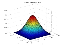
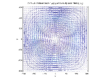
Figure 1: The streamfunction ($\varphi/B$) and the velocity, $v_{\theta}(x,y)$

Physical parameters: $\rho_{s}=0.003\;\left(m\right)$, $L^{phys}=a=1\;\left(m\right)$. After normalization $L=\frac{a}{\rho_{s}}=\frac{1}{0.003}\simeq 330$. The unit of velocity is $c_{s}=9.79\times 10^{3}\sqrt{T_{e}\left(eV\right)}\;\left(m/s\right)$

Numerical solution for $L=307$: dipolar vortex.

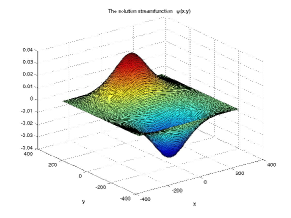
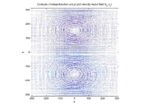
Figure 2: The streamfunction ($\varphi/B$) and the velocity, $v_{\theta}(x,y)$

Numerical solution for $L=307$: quadrupolar vortex.

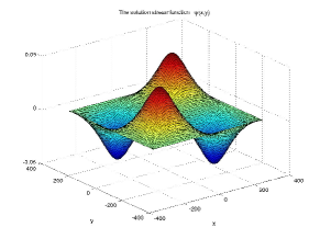
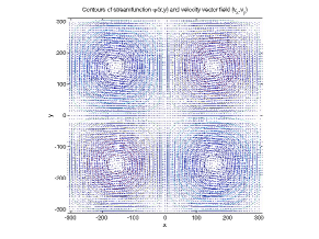
Figure 3: The streamfunction ($\varphi/B$) and the velocity, $v_{\theta}(x,y)$

The amplitudes of the flows is in general small (but not incompatible with the previous analytic results) and should be corrected for the redefinition of the Larmor radius.

9.2 Self-organisation of the drift turbulence

Compare the result from our equation with the result of a statistical/variational theory of drift wave turbulence for the Hasegawa-Wakatani equation.

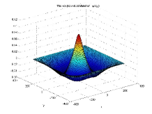
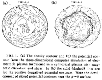
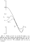
Figure 4: A theory of self-organization of turbulence (Hasegawa-Wakatani) leads to this radial profile for the potential

9.3 The LH transition

We obtain as solution of the Eq.(27) profiles of velocity with a deep drop at the edge. They are similar with the measured profiles observed after the transition L to H.

We must note that the following results are not exact solutions of the Eq.(27). They are approximative solutions,or, in other terms, they verify Eq.(27) only when a larger tolerance is accepted in the GIANT code. Nevertheless, they appear persistently and we can suppose that they correspond not to exact minimum action states, but are local minima of the action or they may have a slow drift in the space of system’s configurations.

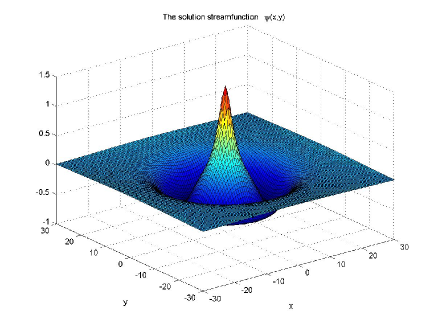
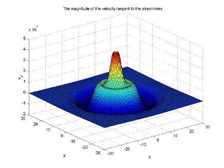
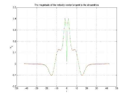
Figure 5: Density series30, set_1.02. $p=1$ and $L=30.$ Here $ampuh=1.02$. The streamfunction $\psi(x,y)$ (f53), the azimuthal velocity $v_{\theta}(x,y)$ (f54) and $v_{\theta}diag$ (f55).

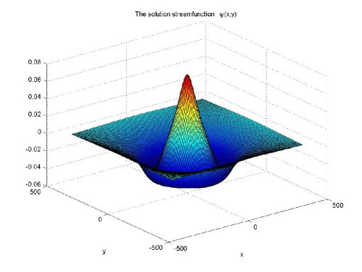
Figure 6: Density, set15_1. $p=1$ and $L=411.$ Streamfunction $\psi$ (f26).

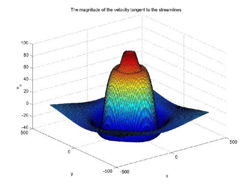
Figure 7: density, set15_1. $p=1$ and $L=411.$ $v_{\theta}$(f27).

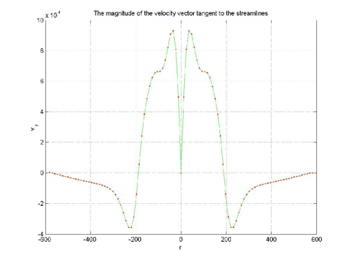
Figure 8: density, set15_1. $p=1$ and $L=411.$ $v_{\theta}$ (f28).

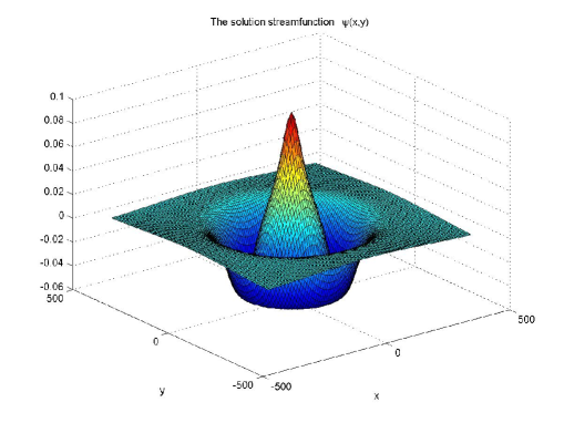
Figure 9: Density, set15_5. $p=1$ and $L=411.$ Streamfunction $\psi$ (f29).

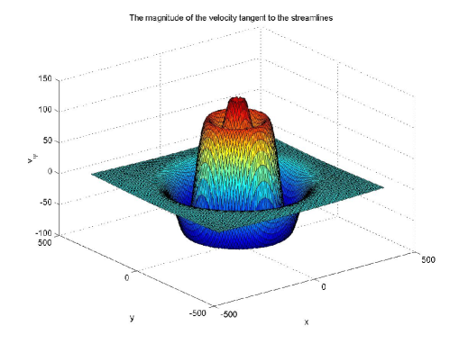
Figure 10: density, set15_5. $p=1$ and $L=411.$ $v_{\theta}$(f30).

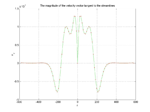
Figure 11: density, set15_5. $p=1$ and $L=411.$ $v_{\theta}$ (f31).

9.3.1 Physical parameters for the H states

The input parameters are

$$a = 1.25\;\left(m\right)$$

$$B_{T} = 2.5\,\left(T\right)$$

From this we can calculate the ion cyclotron frequency

$$\Omega_{ci} = \frac{eB_{T}}{m_{i}}$$

$$= 9.58\times 10^{3}B_{T}\left(Gs\right)$$

$$= 9.58\times 10^{3}\times 25000$$

$$= 239.5\times 10^{6}\left(s^{-1}\right)$$

These are fixed parameters. We need to choose a value for the ion temperature, that will fix the Larmor radius. Take

$$T=2\,(KeV)$$

then

$$c_{s} = 9.79\times 10^{3}\sqrt{T_{e}\left(eV\right)}$$

$$= 4.38\times 10^{5}\,\left(m/s\right)$$

$$\rho_{s} = \frac{c_{s}}{\Omega_{i}}$$

$$= 0.0018\,\left(m\right)$$

This gives

$$L = \frac{a}{\rho_{s}}$$

$$= 682.35$$

The following table shows to what extent we can expect change of the effective (adimensional) length of the integration domain

$T\,\left(KeV\right)$ $\rho_{s}\,\left(m\right)$ $L$ $0.5$ $9.14\times 10^{-4}$ $1367$ $1$ $0.0013$ $967$ $2$ $0.0018$ $683$ $3$ $0.0022$ $558$ $4$ $0.0026$ $483$ $5$ $0.0029$ $432$ $6$ $0.0032$ $395$ $7$ $0.0034$ $365$ $8$ $0.0037$ $341$ $9$ $0.0039$ $322$ $10$ $0.0041$ $306$

A case with $T=5000\,\left(eV\right)$, where $\rho_{s}\simeq 0.003$ and

$$L\simeq 411$$

From the numerical simulations, we have the velocity at the bottom of the region of negative values, close to the border (from the figure f28)

$$v_{\theta,low}\simeq 4\times 10^{-4}$$

The unit of velocity is

$$c_{s} = 9.79\times 10^{3}\sqrt{T_{e}}$$

$$\simeq 7\times 10^{5}\,\left(m/s\right)$$

Then the physical velocity is

$$v_{\theta,low}^{phys}=280\,\left(m/s\right)$$

The radial electric field that can generate this rotation is

$$\frac{E_{r}\left(V/m\right)}{B_{T}\left(T\right)}=v_{\theta}^{phys}\left(m/s\right)$$

or

$$E_{r}=280\times 2.5=700\,\left(V/m\right)$$

9.3.2 Calculation of the radial electric field at the edge

The input parameters are from JET

$$a = 1.\;\left(m\right)$$

$$B_{T} = 2.5\,\left(T\right)$$

From this we can calculate the ion cyclotron frequency

$$\Omega_{ci} = \frac{eB_{T}}{m_{i}}$$

$$= 239.5\times 10^{6}\left(s^{-1}\right)$$

and

$$c_{s}=9.79\times 10^{3}\sqrt{T_{e}}$$

$$\rho_{s}=\frac{c_{s}}{\Omega_{i}}$$

We must use a single value for $T_{e}$ instead of a radial profile. Then the value of $\rho_{s}$ will not be precise. We adopt the point of view that the sonic Larmor radius may be modified by various effects leading to

$$\frac{1}{\rho_{s}^{2}}\rightarrow\frac{1}{\left(\rho_{s}^{eff}\right)^{2}}\equiv\frac{1}{\rho_{s}^{2}}\left(1-\frac{v_{d}}{u}\right)$$

$$v_{d}=\frac{\rho_{s}c_{s}}{L_{n}}$$ (28)

We assume that the system evolves to a state  where two parameters become comparable in magnitude: the velocity of plasma rotation $u$ and the diamagnetic velocity $v_{d}$

$$u\sim v_{d}$$

This is achieved in a structured way, i.e. the various elements behind these parameters evolve individually but in a corralated manner to achieve a new state of equilibrium. The gradient of the density profile $L_{n}$ evolves such that the diamagnetic velocity $v_{d}$ increases on a certain region of plasma, which may be connected with the strong gradient at the pedestal. The plasma poloidal rotation velocity $u$ increases due to the redistribution of vorticity leading to accumulation of vorticity elements toward the center of plasma. It is possible that these parameters attain a relative magnitude such that the effective Larmor radius $\rho_{s}^{eff}$ becomes sufficiently large. This makes possible a new equilibrium of rotation velocity via a new equilibrium vorticity distribution, as a quasi-stationary state. We can take several possible values for them

$$\begin{array}[]{cccccc}v_{d}/u&\rho_{s}^{eff}/\rho_{s}&L=a/\rho_{s}^{eff}&\left|v_{\theta bottom}\right|&\left|v_{\theta bottom}^{phys}\right|\left(m/s\right)&\left|E_{r}\right|(kV/m)\\ 0.2&1.118&273&1\times 10^{-3}&979&2.45\\ 0.4&1.29&236&1\times 10^{-3}&979&2.45\\ 0.85&2.58&95&2.2\times 10^{-3}&2152&5.38\\ 0.95&4.47&63&0.02&19580&48.95\end{array}$$

It stops increasing $\rho_{s}^{eff}$ for a certain ratio $v_{d}/u$.

See below for a more detailed discussion on this topic.

9.4 The density pinch

9.4.1 Introduction

The vorticity $\omega=\mathbf{\nabla}_{\perp}^{2}\phi$ and the particle density $n\left(r,t\right)$ are strongly connected in $2D$ tokamak plasma. Then we must look to the intrinsic evolution of the vorticity profile since from this we can draw conclusions about the density pinch. When we apply the Bogomolnyi procedure to the action functional for $2D$ plasma and atmosphere we find equations describing the stationary states which formally would correspond to self-duality, plus an additional energy which does not have a topological character. We can assume that the equations describe states which are actually quasi-stationary and that the additional (or residual) energy term provides a estimation of the possibility that the system still continues to evolve. This assumption is valid if we can prove that the evolution is slow, which means that the system behaves adiabatically. Although this perspective is not clear yet, we will take it as a basis to investigate the evolution of the vorticity profiles in tokamak, under the field theoretical formulation.

We first recall that in the model of J.B. Taylor of natural current profiles in tokamak it is identified a quantity playing the role of a magnetic temperature for the statistical ensemble of current filaments. This temperature is related with the peaking factor of the profile and it is shown that when the magnetic temperature reaches a critical value, $T_{m}^{c}$, the profile of the current shows a high degree of concentration, in a form of a single current filament on the magnetic axis. This is valid for his statistical (maximum entropy) theory whose analytical result is the Liouville equation for the flux function. However the theory does not provide a physical reason that a possible evolution of the system would consist of an evolution of the magnetic temperature toward the critical value.

In the field theoretical formulation of the same physical model (which also derive the Liouville equation) the physical parameters are $\kappa$ (the coefficient of the Chern-Simons term in the Lagrangian) and the electric charge $e$ (which is actually the elementary current $j_{0}$ of the discrete model). The later can be absorbed into the definition of the potential since the connection between the matter field $\phi$ and the interaction (gauge) potential $A^{\mu}$ needs not be parametrized in any physical way, being established at the level of the discrete model. Therefore the quantity that is still present is $\kappa$. On the other hand, comparing the Taylor model with the field theory model, we find the relationship between the parameters,

$$\left|\kappa\right|=\frac{16\pi e^{2}}{J_{0}^{2}a^{2}c}\frac{1}{T_{m}/T_{m}^{c}-1}$$

from which we see that a very peaked current profile in the form of a concentrated filament, i.e.

$$T_{m}\rightarrow T_{m}^{c}$$

corresponds in field theory to very high values of $\kappa$.

While in the statistical model we cannot find an intrinsic reason for $T_{m}$ to approach (from above) the critical value $T_{m}^{c}$, we can look for the presence of an equivalent tendency in the field theoretical model, asking when there can be reasons for $\kappa$ to increase adiabatically its value.

In the field theoretical model for the $2D$ plasma, where $\kappa$ is identified as the sound speed

$$\kappa\equiv c_{s}=\rho_{s}\Omega_{ci}$$

we can assume that $\kappa$ behaves as $\rho_{s}$, since we take the external confining magnetic field as constant, $B^{ext}=$const. Then an increase of $\kappa$ can result from an increase in $\rho_{s}$.

Physically this is not acceptable when the variation of the temperature is not considered, as was one of our basic assumption. Then what can provide us with an increase of the Larmor radius?

A careful consideration of the physical model underlying the field theoretical formulation may clarify this problem.

The discrete system is based on the idea that elements of vorticity interact on distances of the order of the Larmor radius $\rho_{s}$ (the inverse of the mass of the photon in our theory) and this parameter is taken constant throughout. However in the plasma there is another ‘field’ that has a strong connection with the vorticity: the density $n\left(\mathbf{r},t\right)$. Due to the compressibility of the ion polarization drift velocity, the density is not constant in the CHM plasma (as opposed to the Euler fluid case). The spatial variation of the density (i.e. $L_{n}\neq\infty$) is the cause for the diamagnetic flow with the velocity $v_{dia}=\rho_{s}c_{s}/L_{n}$. The interaction between point-like vortices of the discrete model adapts itself to the presence of two velocities: one is the velocity $u$, simply associated with the vorticity, with which the cluster of point-like vortices (i.e. the physical vorticity) is in the relationship $\mathbf{\omega}=\mathbf{\nabla\times u}$. The other is the diamagnetic velocity of the plasma, $v_{dia}$ essentially induced by density gradients. The distance of interaction between two elementary vortices is modified with the factor

$$\left(1-\frac{v_{dia}}{u}\right)^{-1}$$

since this has been proven that affects directly the Larmor radius, replacing the physical parameter $\rho_{s}$ with an effective one, $\rho_{s}^{eff}$,

$$\frac{1}{\left(\rho_{s}^{eff}\right)^{2}}=\frac{1}{\rho_{s}^{2}}\left(1-\frac{v_{dia}}{u}\right)$$

It is this quantity that appears systematically when vortical motion is examined in tokamak plasma, as illustrated below by the treatment for a drift wave vortex.

Then we should accept that our field theoretical formulation, based on a constant $\rho_{s}$ can only be valid on small patches, and there, with actually the effective Larmor radius. Then we have that the parameter $\kappa$, the coefficient of the Chern-Simons term in Lagrangian, has a “slow” spatial variation coming from the spatial variation of $\rho_{s}^{eff}$, which, in turn is given by the difference between the plasma rotation velocity $u$ and the ion diamagnetic velocity $v_{dia}$.

The first conclusion that we can draw at this moment is that an evolution of the density profile that leads to an increase of the gradient (i.e. $L_{n}$ smaller) will increase the diamagnetic velocity and then $v_{dia}$ tends to approach from below the plasma rotation velocity $u$. In consequence the factor $\left(1-\frac{v_{dia}}{u}\right)$ becomes smaller and the effective Larmor radius increases. This is translated in the field theoretical model in an increase of $\kappa$. If we follow the analogy presented above, according to which the increase of $\kappa$ is equivalent to $T_{m}\searrow T_{m}^{c}$, we find that there is an enhanced clusterization of the elements of vorticity, with a possible evolution toward a single filament in the center.

This process is not stationary since it has a positive feedback: the clusterization of the vorticity toward the center drags the density (basically from Ertel’s theorem, but the process is more complex) and the evolution of the density increases the gradient and consequently the diamagnetic velocity. The effective Larmor radius increases and the parameter $\kappa$ increases which still enhances the clusterization process for the vortical elements.

However there is a limit to this process, coming exactly from the same reason for which the vorticity and the density evolve together and exhibit an inward pinch in tokamak.

The limit consists of the fact that the factor $1-v_{dia}/u$ ends up by saturating the process of pinching, due to a too large increase of the effective Larmor radius.

When the effective Larmor radius is too big, the interaction between the elements of vorticity is no more of short range but can be considered of long range. Or, this is the case of the Euler fluid, where the range of interaction is Coulombian (i.e. $ln$). For the Euler fluid there is no compressibility of the background density, the density and the vorticity are decoupled and the density cannot follow the vorticity. The compressibility of the ion polarization drift is proportional with the inverse of the square of the effective Larmor radius and this diminishes accordingly. The fluid becomes less Hasegawa-Mima and more Euler. Actually the state where $v_{dia}=u$ corresponds exactly to the two fluids: Hasegawa-Mima (because the density is adiabatic and then $v_{dia}=u$) and Euler (since there the range of interaction is infinite, Coulombian). But the directions from which the two fluids arrive at this state are completely different.

This intuitive representation of the density pinch (via the vorticity pinch) may be useful. However the field theory introduces an additional factor in this model: the fact that intrinsically the quasi-self-dual solutions have an adiabatic evolution related with the existence of a residual energy which is not of a topological nature.

For the Eq.(27) the residual energy puts severe limitations to the increase of the normalized value of the streamfunction. Any $\psi$ that is greater than $\sim 3$ is strongly inhibited by a severe increase of this residual energy. Or, the concentration in the center of the vorticity is in general accompanied by an increase of $\psi$. We should note however that for a normalized domain of integration $L=L^{phys}/\rho_{s}^{eff}$ of the order greater than $\sim 10$ the value of $\psi$ is already smaller than $1$, and the limitations imposed by the residual energy are far. Moreover, the graph of this residual energy shows that there is a favorable slow evolution for the small values of $\psi$ since close to $\psi=0$ the energy is decreasing with increasing $\psi$.

We still have to work on that.

9.4.2 The role of the effective Larmor radius $\rho_{s}^{eff}$

In Stationary vortices drift waves (Nycander) it is derived the equation

$$\Delta\phi=\left(\frac{1}{u}\frac{n_{0}^{\prime}}{n_{0}}+\frac{1}{\tau\left(x\right)}\right)\phi$$

where

$$\tau\left(x\right)\equiv\frac{T_{e}\left(x\right)}{T_{0}}$$

and the normalizations are usual: $\rho_{s}$ , $\Omega_{i}$ and $e/T_{e}$ for space, time, potential. From here we derive, taking constant temperature

$$\frac{1}{u}\frac{n_{0}^{\prime}}{n_{0}}+\frac{1}{\tau\left(x\right)} = \frac{1}{u^{phys}\left(\frac{\Omega_{i}}{\rho_{s}}\right)}\frac{1}{n_{0}}\frac{dn_{0}}{dr^{phys}/\rho_{s}}+1$$

$$= \frac{\rho_{s}^{2}}{\Omega_{i}}\left(\frac{dn_{0}}{n_{0}dr}\right)^{phys}\frac{1}{u}+1$$

$$= 1+\frac{c_{s}\rho_{s}}{\Omega_{i}}\frac{1}{L_{n}}\frac{1}{u}$$

$$= 1-\frac{v_{d}}{u}$$

where we defined

$$v_{d}\equiv-\frac{c_{s}\rho_{s}}{\Omega_{i}}\frac{1}{L_{n}}$$

such that when

$$L_{n}<0$$

we have

$$v_{d}>0$$

The two velocities, $v_{d}$ and $u$ are in the same direction (positive) when the density decreases radially, which is normal in tokamak. Therefore we have that

$$1-\frac{v_{d}}{u}>0$$

if the velocity of plasma rotation is higher than the diamagnetic rotation. When the diamagnetic rotation becomes comparable with the plasma rotation velocity, just slightly lower, this factor is almost zero and the effective Lamor radius becomes infinite.

10 Conclusions

This work is intended to provide arguments in favor of validity and usefulness of the Field Theoretical approach to the description of fluids and plasmas in the evolution towards asymptotic, coherent structures.

The basis material consisting of definition of the Lagrangians, equations of motion and Self-Duality states are presented elsewhere and is not mentioned here. The applications are only shortly presented.

We focused on various instruments, like the field-theoretical currents, energy and action functional in close proximity of the self-duality. We have noted that there are important aspects that can be examined using these instruments, specific to the field theory:

• the existence of the current of point-like vortices, which can explain the concentration of vorticity

• the slowing down of the evolution in the cuasi-asymptotic state, where the number of vortices is still not the minimum that is obtained as the pure extremum of the action at self-duality

• the importance of parameters like the coefficient of the Chern-Simons factor, in the adiabatic change of the regimes;

• the role of the effective spatial dimension, which is adjusted spontaneously via the gradients of the vorticity field.

Much remains to be investigated but there are already reasons to develop the field theoretical formulations in a large class of fluid and plasma problems.

Acknowledgement 1

This work has been supported by the Romanian Ministry of Education and Research under Ideas Exploratory Research Project No.557

References

- [1] W.H. Matthaeus, W.T. Stribling, D. Martinez, S. Oughton and D. Montgomery, Phys. Rev. Lett. 66, 2731 (1991).
- [2] W.H. Matthaeus, W.T. Stribling, D. Martinez, S. Oughton and D. Montgomery, Physica D51, 531 (1991).
- [3] R. Kinney, J. C. McWilliams and T. Tajima, Phys. Plasmas 2, 3623 (1995).
- [4] W. Horton and A. Hasegawa, Chaos 4, 227 (1994).
- [5] R. H. Kraichnan and D. Montgomery, Rep. Prog. Phys. 43, 547 (1980).
- [6] G. Joyce and D. Montgomery, J. Plasma Phys. 10, 107 (1973).
- [7] D. Montgomery, W.H. Mathaeus, W.T. Stribling, D. Martinez and S. Oughton, Phys. Fluids A4, 3 (1992).
- [8] F. Spineanu and M. Vlad, Phys. Rev.E 67, 046309 (2003).
- [9] J. G. Charney, Geophys. Public. Kosjones Nors. Videnshap. Akad. Oslo, 17, 3 (1948).
- [10] A. Hasegawa and K. Mima, Phys. Fluids 21, 87 (1978).
- [11] F. Spineanu, and M. Vlad, Phys.Rev.Lett. 94, 235003-1 (2005).
- [12] F. Spineanu and M. Vlad, arXiv.org/physics/0501020.
- [13] F. Spineanu and M. Vlad, arXiv.org/physics/0503155.
- [14] F. de Rooij, P. F. Linden and S. B. Dalziel, J. Fluid Mech. 383, 249 (1999).
- [15] C. E. Seyler, J. Plasma Phys. 56, 553 (1996).
- [16] H.E. Willoughby, and P.G. Black, Bull. Amer. Meteor. Soc. 77, 543 (1996).
- [17] Y. Wang, and C.-C. Wu C.-C., Meteorol. Atmos. Phys. 87, 257 (2004).
- [18] P.D. Reasor, and M.T. Montgomery, J. Atmos. Sci. 58, 2306 (2001).
- [19] J.P. Kossin and W.H. Schubert, J. Atmos. Sci. 58, 2196 (2001).
- [20] K.A. Emanuel, J. Atmos. Sci. 43, 585 (1986).
- [21] K.A. Emanuel, J. Atmos. Sci. 43, 3431 (1989).
- [22] M.V. Nezlin, G.P. Chernikov, A.Y. Rylov, K.B. Titishov, Chaos 6, 309 (1996).
- [23] R.S. MacKay, Slow Manifolds, in Energy Localization and Transfer, Eds. T. Dauxois, A. Litvak-Hinenzon, R.S. MacKay, A. Spanoudaki (World Scientific, 2004), 149.
- [24] J.P. Boyd, Dyn. Atmos. Oceans, 22, 49 (1995).
- [25] Typhoon database at the web address: http://agora.ex.nii.ac.jp/digital-typhoon.
- [26] G. K. Morikawa, Journal of Meteorology 17, 148 (1960).
- [27] H. J. Stewart, Q. Appl. Math. 1, 262 (1943).
- [28] U. Nowak, and L. Weimann, GIANT A software package for the numerical solution of very large systems of highly nonlinear equations, Konrad-Zuse-Zentrum fur Informationtechnik Berlin, Technical Report TR 90-11 (1990).
- [29] F. Spineanu, M. Vlad, K. Itoh, H. Sanuki and S.-I. Itoh, Phys. Rev. Lett. 93, 025001-1 (2004).
- [30] G. J. Holland, Mon. Wea. Rev. 108, 1212 (1980).
- [31] M. DeMaria, J.A. Knaff, J. Dostalek, K.J. Mueller, ”Improvement in deterministics and probabilistic tropical cyclone wind prediction”, presented at ”The Inter-Departamental Hurricane Conference”, Charleston (USA) (2004).
- [32] F. Spineanu and M. Vlad, Geophysical and Astrophysical Fluid Dynamics, 103, 223 (2009).