Loop Quantum Cosmology on a Torus

Abstract

In this paper we study the effect of a torus topology on Loop Quantum Cosmology. We first derive the Teichmüller space parametrizing all possible tori using Thurston’s theorem and construct a Hamiltonian describing the dynamics of these torus universes. We then compute the Ashtekar variables for a slightly simplified torus such that the Gauss constraint can be solved easily. We perform a canonical transformation so that the holomies along the edges of the torus reduce to a product between almost and strictly periodic functions of the new variables. The drawback of this transformation is that the components of the densitized triad become complicated functions of these variables. Nevertheless we find two ways of quantizing these components, which in both cases leads surprisingly to a continuous spectrum.

1 Introduction

The Einstein field equations are local equations in the sense that they only describe the local geometry of the spacetime. For example the Robertson-Walker metric explicitly contains the parameter $k$ which gives an account of the intrinsic spatial curvature. Using the Friedmann equations this parameter can be determined experimentally since it is directly related to the density parameter $\Omega_{\mathrm{tot}}$ and the Hubble parameter $h$. Recent measurements of the energy density of the universe tend to slightly favor a positively curved universe [1], yet a flat curvature lies within the 1-$\sigma$ range. The most direct conclusion is that the spatial topology of the universe is just $\mathds{R}^{3}$ which is the assumption of the $\Lambda$CDM model. Nevertheless in the mathematical literature it is well known that a flat space does not mean that its topology is necessarily $\mathds{R}^{3}$, in fact there are 18 possible flat topologies. Since the Einstein field equations are not sensitive to topology every possibility has to be considered as a possible candidate for the global geometry of our universe until it is ruled out by experiment. In order to do so we first note that the spectrum of the Laplace operator sensitively depends on the topology, i.e. it is discrete if the eigenstates are normalizable and continuous if not. In the first case the solution for e.g. a torus is given by plane waves with a wave vector $\vec{k}_{n}$ taking only discrete values $n\in\mathds{N}$ while in the second case the (weak) solution to the eigenvalue equation is given by the (distributional) plane waves with a continuous wave vector $\vec{k}$. For example, the eigenvalue problem for $\triangle$ on $\mathds{T}^{3}$ is given by $(\triangle+E_{\vec{n}})\Psi_{\vec{n}}=0,\;\vec{n}\in\mathds{N}^{3}$, and on $S^{3}$ by $\triangle\Psi_{\beta,l,m}=(\beta^{2}-1)\Psi_{\beta,l,m},$ where $\beta\in\mathds{N}$, $0\leq l\leq\beta-1$ and $|m|\leq l$. The implication of a solution of the form $\Psi_{\vec{n}}$ is the existence of a wave function $\Psi_{n}$ with a maximum length corresponding to e.g. the length of the edges of the torus. Since the departure from a continuous solution is biggest for large wavelengths we have to look for large-scale structures of the universe in order to distinguish between cosmic topologies. The best way to do so is to measure the inhomogeneities of the cosmic microwave background (CMB), expand these in multipole moments and compare the low multipoles with the predictions from theory. It can be shown that in certain closed topologies a suppression in the power spectrum of the low multipoles is expected because of the existence of a largest wavelength. Since such a suppression is present in the CMB several studies compared the theoretical predictions for various topologies with the data. While most analyzed topologies can already be ruled out three of them describe the data even better than the infinite $\Lambda$CDM model, namely the torus [2, 3, 4], the dodecahedron[5, 6] and the binary octahedron[7] (see also references therein). While the last two topologies are spherical the torus is the simplest model of a closed flat topology.

However, we know that standard cosmology cannot be the final answer as its predictability breaks down at the big bang. A quantization of the Friedmann equations a la Wheeler-DeWitt does not improve this behavior either. This situation has changed thanks to a new model called loop quantum cosmology (LQC) developed over the last few years which removes the initial singularity. LQC [8, 9, 10, 11, 12, 13, 14, 15, 16] is the approach motivated by loop quantum gravity (LQG) [17, 18, 19] to the quantization of symmetric cosmological models. The usual procedure is to reduce the classical phase space of the full theory to a phase space with a finite number of degrees of freedom. The quantization of these reduced models uses the tools of the LQG and is therefore called LQC but it does not correspond to the cosmological sector of LQG. The results of LQC not only provide new insights into the quantum structure of spacetime near the Big-Band singularity but also remove this singularity by extending the time evolution to negative times.

In sum, on the one hand we have hints from observation that our universe may have a closed topology, on the other hand we have a very successful loop quantization of various cosmologies. Thus, starting from these two motivations, we would like to study LQC with a torus topology. But contrary to the works on the CMB we don’t want to restrict the analysis to a cubical torus. To do so we construct a torus using Thurston’s theorem and find that the most general torus has six degrees of freedom which consist of e.g. three lengths and three angles. We will study its dynamics by numerically solving the Hamiltonian coupled to a scalar field. After rewritting this Hamiltonian in terms of Ashtekar variables we will see that the quantization of such a torus leads to a product between the standard Hilbert spaces of LQC and the Hilbert spaces over the circle. Moreover, we will find two ways to quantize the components of the triad and show that both (generalized) eigenfunctions are not normalizable in this Hilbert space.

As a side remark we would like to point out that the consequences of putting a non-abelian gauge theory into a box with periodic boundary conditions have been studied in e.g. [20]. The motivation behind this idea is an attempt to explain the quark confinement in QCD without explicitely breaking gauge invariance. To simplify the analysis the $su(N)$-valued gauge field is chosen to be pure gauge, i.e. $A=U^{-1}dU$ with $U\in SU(N)$, such that the holonomy around a closed curve $C$ only depends on the topological property of $C$. Since general relativity written in terms of Ashtekar variables is also a (constrained) Yang-Mills theory it may be tentalizing to use the methods developed for QCD in a box to LQC of a torus universe. However we will derive an Ashtekar connection for the homogeneous torus which is not pure gauge so that the holonomies along $C$ also depend on the length of $C$. This may not be surprising in view of the fact that the Hilbert space of LQC on $\mathds{R}^{3}$ is spanned by almost periodic functions with an arbitrary length parameter $\mu$.

This paper is organized as follows: in Section 2 we first introduce the classical dynamics of a torus universe and numerically solve the Friedmann equations with a massless scalar field. In Section 3 we introduce the Ashtekar variables for a torus and also explain the complications that arise because of a closed topology. The loop quantization and the construction of a Hilbert space are explained in Section 4 and Section 5 provides a summary and directions for future works. A gives a short review of the fundamental domain of the 3-torus and B describes the dynamics of the torus in terms of Iwasawa coordinates.

2 Compact Homogeneous Universes and their Dynamics

The purpose of this section is to study models in which the spatial section has a compact topology. The compactness of a locally homogeneous space brings new degrees of freedom of deformations, known as Teichmüller deformations. This leads to the conclusion that cosmology on a torus is simply cosmology on $\mathds{R}^{3}$ restricted to a cube may be too naive a point of view, especially since the space of solutions of a torus gets nine additional degrees of freedom, as already mentioned in [21]. We will introduce Teichmüller spaces with an emphasis on a Thurston geometry admitting a Bianchi I geometry as its subgeometry [22, 23, 24, 25, 26] and derive the vacuum Friedmann equations using the Hamiltonian formalism.

2.1 Compact Homogeneous Spaces

Let $\Sigma$ be a three-dimensional, arcwise connected Riemannian manifold.

Definition 1.

A metric on a manifold $\Sigma$ is locally homogeneous if $\forall p,q\in\Sigma$ there exist neighborhoods $U,V$ of $p$ resp. $q$ and an isometry $(U,p)\rightarrow(V,q)$. The manifold is globally homogeneous if the isometry group acts transitively on the whole manifold $\Sigma$.

Since $\Sigma$ is arcwise connected we know that there is a unique universal covering manifold $\tilde{\Sigma}$ up to diffeomorphisms with a metric given by the pullback of the metric on $\Sigma$ by the covering map

$$\pi:\tilde{\Sigma}\rightarrow\Sigma.$$ (1)

Singer [27] proved that the metric on $\tilde{\Sigma}$ is then globally homogeneous and $\tilde{\Sigma}$ is given by $\tilde{\Sigma}\cong\tilde{S}/F$, where $\tilde{S}$ is the orientation preserving isometry group of $\tilde{\Sigma}$ and $F$ its isotropy subgroup.

On the other hand, we can also start from a three-dimensional, simply connected Riemannian manifold $\tilde{\Sigma}$ which admits a compact quotient $\Sigma$. In order to construct this compact manifold consider the covering group $\Gamma\subset\tilde{S}$ which is isomorphic to the fundamental group $\pi_{1}(\Sigma)$ of $\Sigma$. This implies that

$$\Sigma=\tilde{\Sigma}/\Gamma,$$

which is Hausdorff iff $\Gamma$ is a discrete subgroup of $\tilde{S}$ and a Riemannian manifold iff $\Gamma$ acts freely on $\tilde{\Sigma}$.

Definition 2.

A geometry is the pair $(\tilde{\Sigma},S)$ where $\tilde{S}$ a group acting transitively on $\tilde{\Sigma}$ with compact isotropy subgroup. A geometry $(\tilde{\Sigma},\tilde{S}^{\prime})$ is a subgeometry of $(\tilde{\Sigma},\tilde{S})$ if $\tilde{S}^{\prime}$ is a subgroup of $\tilde{S}$. A geometry $(\tilde{\Sigma},\tilde{S})$ is called maximal if it is not a subgeometry of any geometry and minimal if it does not have any subgeometry.

We will need the following important theorem:

Theorem 1 (Thurston [28]).

Any maximal, simply connected 3-dimensional geometry which admits a compact quotient is equivalent to the geometry $(\tilde{\Sigma},\tilde{S})$ where $\tilde{\Sigma}$ is one of $E^{3}$ (Euclidean), $H^{3}$ (hyperbolic), $S_{p}^{3}$ (3-sphere), $S_{p}^{2}\times\mathds{R}$, $H^{2}\times\mathds{R}$, $\widetilde{SL}(2,\mathds{R})$, Nil or Sol.

If $(\tilde{\Sigma},\tilde{S}^{\prime})$ is not a maximal geometry but is simply connected and admits a compact quotient as well we can find a discrete subgroub $\Gamma^{\prime}$ of $\tilde{S}^{\prime}$ acting freely so as to make $\tilde{\Sigma}/\Gamma^{\prime}$ compact. Define $(\tilde{\Sigma},\tilde{S})$ as the maximal geometry with $(\tilde{\Sigma},\tilde{S}^{\prime})$ as its subgeometry, i.e. $\tilde{S}^{\prime}\subset\tilde{S}$. By Thurston’s Theorem $(\tilde{\Sigma},\tilde{S})$ is one of the eight Thurston geometries, which implies that $(\tilde{\Sigma},\tilde{S}^{\prime})$ is a subgeometry of one of the eight Thurston geometries.

Theorem 2.

Any minimal, simply connected three-dimensional geometry is equivalent to $(\tilde{\Sigma},\tilde{S})$, where $\tilde{\Sigma}=\mathds{R}^{3}$, $\tilde{S}=$Bianchi I-VIII; $\tilde{\Sigma}=S_{p}^{3}$, $\tilde{S}=$Bianchi IX; or $\tilde{\Sigma}=S_{p}^{2}\times\mathds{R}$, $\tilde{S}=SO(3)\times\mathds{R}$, where $S_{p}^{3}$ is the three-sphere and $S_{p}^{2}$ the two-sphere.

Let Rep$(\Sigma)$ denote the space of all discrete and faithful representations $\rho:\pi_{1}(\Sigma)\rightarrow\tilde{S}$ and the diffeomorphism $\phi:\tilde{\Sigma}\rightarrow\tilde{\Sigma}$ a global conformal isometry if $\phi_{*}\tilde{h}_{ab}=\mathrm{const}\cdot\tilde{h}_{ab}$, where $\tilde{h}_{ab}$ is the spatial metric of the universal covering manifold $\tilde{\Sigma}$. This allows us to define a relation $\rho\sim\rho^{\prime}$ in Rep$(\Sigma)$ if there exists a conformal isometry $\phi$ of $\tilde{\Sigma}$ connected to the identity with $\rho^{\prime}(a)=\phi\circ\rho(a)\circ\phi^{\prime}$.

Definition 3.

The Teichmüller space is defined as

$$\mathrm{Teich}(\Sigma)=\mathrm{Rep}(\Sigma)/\sim$$

with elements called Teichmüller deformations, which are smooth and nonisometric deformations of the spatial metric $h_{ab}$ of $\Sigma$, leaving the universal cover $(\tilde{\Sigma},\tilde{h}_{ab})$ globally conformally isometric.

The situation gets more complicated when we try to extend the previous construction to four-dimensional Lorentzian manifolds. The reason is that the action of the covering group $\Gamma$ needs to preserve both the extrinsic curvature and the spatial metric of $\tilde{\Sigma}$. Thus we cannot construct a homogeneous compact manifold by the action of a discrete subgroup of $\tilde{S}$ on the spatial three-section $\tilde{\Sigma}$. Instead we need the isometry group of the four-dimensional manifold $\tilde{M}$. Let $M=\mathds{R}\times\Sigma$ be a compact homogeneous Lorentzian manifold with metric $g_{\mu\nu}$ and $\tilde{M}=\mathds{R}\times\tilde{\Sigma}$ its covering with metric $\tilde{g}_{\mu\nu}$ $(\mu,\nu=0,\ldots,4)$.

Definition 4.

Let $(\tilde{\Sigma},\tilde{h}_{ab})$ be a spatial section of $(\tilde{M},\tilde{g}_{\mu\nu})$. An extendible isometry is defined by the restriction of an isometry of $(\tilde{M},\tilde{g}_{ab})$ on $\tilde{\Sigma}$ which preserves $\tilde{\Sigma}$ and forms a subgroup $\mathrm{Esom}(\tilde{\Sigma})$ of $\tilde{S}$.

Thus, in order to get a compact homogeneous manifold from $\tilde{M}$ the covering group $\Gamma$ must be a subgroup of Esom$(\tilde{\Sigma})$, i.e.

$$\Gamma\subset\mathrm{Esom}(\tilde{\Sigma}).$$

The line element of $M=\mathds{R}\times\Sigma$ is given by

$$ds^{2}=-dt^{2}+h_{ab}(t)\sigma^{a}\sigma^{b},$$

where $\sigma^{a}$ are the invariant one-forms.

Therefore the Teichmüller parameters enlarge the parameter space by bringing new degrees of freedom from the deformations defined in Definition 3. In fact, the set of all possible universal covers $(\tilde{M},\tilde{g}_{ab})$ carries the degrees of freedom of the local geometry and the covering maps $\Gamma$ the degrees of freedom of the global geometry which are parameterized by the Teichmüller parameters.

2.2 The Torus Universe

In this section we restrict the above analysis to the case of a flat torus and give only the main results. Further details can be found in [22, 23, 24, 25, 26]. Let $\tilde{M}=\mathds{R}\times\tilde{\Sigma}$ be the universal cover of $M$ and $\tilde{\Sigma}$ the Thurston geometry $(E^{3},ISO(3,\mathds{R}))$. The isometry group $ISO(3)$ is expressed as $g(\mathbf{x})=\mathbf{Rx}+\mathbf{a}$, where $\mathbf{a}$ is a constant vector and $\mathbf{R}\in SO(3)$ in order that the orientation be preserved. The Killing vectors of $E^{3}$ are

$$\xi_{1}=\partial_{x},\quad\xi_{2}=\partial_{y},\quad\xi_{3}=\partial_{z},$$

$$\xi_{4}=-z\partial_{y}+y\partial_{z},\quad\xi_{5}=-x\partial_{z}+z\partial_{x},\quad\xi_{6}=-y\partial_{x}+x\partial_{y}.$$

The line element of $\tilde{M}$ is thus given by

$$ds^{2}=-dt^{2}+\tilde{h}_{ab}dx^{a}dx^{b}=-dt^{2}+a^{2}(t)\,^{0}\tilde{h}_{ab}dx^{a}dx^{b},$$

where $\,{}^{0}\tilde{h}_{ab}$ is called the fiducial metric in the LQC literature and $dx^{a}$ are the invariant one-forms of the group $ISO(3,\mathds{R})$ .

Figure 1: The vectors $a_{1}$, $a_{2}$ and $a_{3}$ span the torus with six Teichmüller parameters. The global conformal invariance was used in order to align $a_{1}$ with $\xi_{1}$ and $a_{2}$ with span$\{\xi_{1},\xi_{2}\}$.

The covering group $\Gamma\subset\mathrm{Esom}(\tilde{\Sigma})\equiv\mathrm{Esom}(E^{3})$ allows us to construct a torus via $M=\tilde{M}/\Gamma$, where $M=\mathds{R}\times\mathds{T}^{3}$. The freedom of global conformal transformations allows us to choose the coordinate system of $\tilde{\Sigma}$ such that the generators of the torus have a simple representation. We thus require one of the generators to be aligned with $\xi_{1}$ and one to lie in the $\xi_{1}\xi_{2}$-plane. The Teichmüller space is then generated by six Teichmüller parameters in three vectors

$$a_{1}=\left(\begin{array}[]{c}a_{1}\,^{1}\\ 0\\ 0\end{array}\right),\quad a_{2}=\left(\begin{array}[]{c}a_{2}\,^{1}\\ a_{2}\,^{2}\\ 0\end{array}\right),\quad a_{3}=\left(\begin{array}[]{c}a_{3}\,^{1}\\ a_{3}\,^{2}\\ a_{3}\,^{3}\end{array}\right),$$ (2)

where all $a_{i}\,^{j}$ only depend on the coordinate time $t$. The configuration space $\mathcal{C}$ is therefore spanned by the six Teichmüller parameters such that $\mathcal{C}\subset\mathds{R}^{6}$ (see A). The flat spatial metric on $\mathds{T}^{3}$ is then given by $(a,b=1,2,3)$

$$ds^{2}=h_{ab}dx^{a}dx^{b},\quad h_{ab}=\sum_{c}a_{a}\,^{c}a_{b}\,^{c}$$ (3)

where

$$(h_{ab})=\left(\begin{array}[]{ccc}(a_{1}\,^{1})^{2}&a_{1}\,^{1}a_{2}\,^{1}&a_{1}\,^{1}a_{3}\,^{1}\\ &(a_{2}\,^{1})^{2}+(a_{2}\,^{2})^{2}&a_{2}\,^{1}a_{3}\,^{1}+a_{2}\,^{2}a_{3}\,^{2}\\ \mathrm{(sym)}&&(a_{3}\,^{1})^{2}+(a_{3}\,^{2})^{2}+(a_{3}\,^{3})^{2}\end{array}\right).$$ (4)

This metric is invariant under transformations in $SL(3,\mathds{Z})$. For example it is left invariant by $(a_{1}\,^{1}\rightarrow-a_{1}\,^{1},a_{2}\,^{1}\rightarrow-a_{2}\,^{1},a_{3}\,^{1}\rightarrow-a_{3}\,^{1})$ (see A for more details). From Equation (4) we can make a Legendre transform of the Einstein-Hilbert action

$$S_{\mathrm{E-H}}[g]=\frac{1}{2\kappa}\int_{\mathds{R}\times\mathds{T}^{3}}*R[g],\quad\kappa=8\pi G$$ (5)

to obtain a Hamiltonian, where $*$ is the Hodge star operator. After a partial integration of $\ddot{a}_{i}\,^{i}$ (which also cancels the surface term we omitted in Equation (5)) we find the following Lagrangian:

$$\mathcal{L}= \frac{1}{4\kappa}\frac{1}{a_{1}\,^{1}a_{2}\,^{2}a_{3}\,^{3}}\times$$

$$\biggl{[} \left((a_{3}\,^{2})^{2}+(a_{3}\,^{3})^{2}\right)\left(a_{2}\,^{1}\dot{a}_{1}\,^{1}-a_{1}\,^{1}\dot{a}_{2}\,^{1}\right)^{2}+(a_{1}\,^{1})^{2}(a_{3}\,^{2})^{2}(\dot{a}_{2}\,^{2})^{2}$$

$$+ (a_{2}\,^{2})^{2}\Bigl{\{}(a_{3}\,^{1})^{2}(\dot{a}_{1}\,^{1})^{2}-2a_{1}\,^{1}a_{3}\,^{1}\dot{a}_{1}\,^{1}\dot{a}_{3}\,^{1}$$

$$\quad\quad\quad+a_{1}\,^{1}\Bigl{(}a_{1}\,^{1}\left((\dot{a}_{3}\,^{1})^{2}+(\dot{a}_{3}\,^{2})^{2}\right)-4a_{3}\,^{3}\dot{a}_{1}\,^{1}\dot{a}_{3}\,^{3}\Bigr{)}\Bigr{\}}$$

$$- 2a_{2}\,^{2}\Bigl{\{}a_{2}\,^{1}a_{3}\,^{2}\dot{a}_{1}\,^{1}\left(a_{3}\,^{1}\dot{a}_{1}\,^{1}-a_{1}\,^{1}\dot{a}_{3}\,^{1}\right)$$

$$\quad\quad\quad+a_{1}\,^{1}\Bigl{[}a_{1}\,^{1}a_{3}\,^{2}\dot{a}_{2}\,^{1}\dot{a}_{3}\,^{1}-a_{3}\,^{1}a_{3}\,^{2}\dot{a}_{1}\,^{1}\dot{a}_{2}\,^{1}$$

$$\quad\quad\quad\quad\quad\quad+\dot{a}_{2}\,^{2}\left(a_{1}\,^{1}a_{3}\,^{2}\dot{a}_{3}\,^{2}+2a_{3}\,^{3}(a_{3}\,^{3}\dot{a}_{1}\,^{1}+a_{1}\,^{1}\dot{a}_{3}\,^{3})\right)\Bigr{]}\Bigr{\}}\biggl{]}$$

We introduce the momenta

$$p^{a}\,_{b}:=\frac{\partial\mathcal{L}}{\partial\dot{a}_{a}\,^{b}}$$ (6)

conjugate to the configuration variables $a_{a}\,^{b}$ such that the phase space $\mathcal{P}=T^{*}\mathcal{C}\subset\mathds{R}^{12}$ is the cotangent bundle over $\mathcal{C}$ with

$$\{a_{a}\,^{b},p^{c}\,_{d}\}=\delta_{a}^{c}\delta^{b}_{d},\quad\{a_{a}\,^{b},a_{c}\,^{d}\}=0,\quad\{p^{a}\,_{b},p^{c}\,_{d}\}=0,$$ (7)

where the Poisson brackets are defined as

$$\{f,g\}=\sum_{a,b=1}^{3}\frac{\partial f}{\partial a_{a}\,^{b}}\frac{\partial g}{\partial p^{a}\,_{b}}-\frac{\partial g}{\partial a_{a}\,^{b}}\frac{\partial f}{\partial p^{a}\,_{b}}$$

for any smooth functions on the phase space. We insert $\dot{a}_{a}\,^{b}=\dot{a}_{a}\,^{b}(p^{c}\,_{d})$ into the Legendre transform of Equation (5) and get the Hamiltonian

$$\mathcal{H}_{g}= \frac{\kappa}{4}\frac{1}{a_{1}\,^{1}a_{2}\,^{2}a_{3}\,^{3}}\times$$

$$\biggl{[} (a_{1}\,^{1}p^{1}\,_{1})^{2}+(a_{2}\,^{2}p^{2}\,_{2})^{2}+(a_{3}\,^{3}p^{3}\,_{3})^{2}+(a_{2}\,^{1}p^{2}\,_{1})^{2}+4(a_{2}\,^{2}p^{2}\,_{1})^{2}$$

$$+ (a_{3}\,^{1}p^{3}\,_{1})^{2}+4(a_{3}\,^{2}p^{3}\,_{1})^{2}+4(a_{3}\,^{3}p^{3}\,_{1})^{2}+(a_{3}\,^{2}p^{3}\,_{2})^{2}$$

$$+ 4(a_{3}\,^{3}p^{3}\,_{2})^{2}-2a_{3}\,^{2}a_{3}\,^{3}p^{3}\,_{2}p^{3}\,_{3}$$

$$+ 2a_{1}\,^{1}p^{1}\,_{1}\left(a_{2}\,^{1}p^{2}\,_{1}-a_{2}\,^{2}p^{2}\,_{2}+a_{3}\,^{1}p^{3}\,_{1}-a_{3}\,^{2}p^{3}\,_{2}-a_{3}\,^{3}p^{3}\,_{3}\right)$$

$$- 2a_{3}\,^{1}p^{3}\,_{1}\left(a_{3}\,^{2}p^{3}\,_{2}+a_{3}\,^{3}p^{3}\,_{3}\right)$$

$$- 2a_{2}\,^{1}p^{2}\,_{1}\left(a_{2}\,^{2}p^{2}\,_{2}-a_{3}\,^{1}p^{3}\,_{1}+a_{3}\,^{2}p^{3}\,_{2}+a_{3}\,^{3}p^{3}\,_{3}\right)$$

$$+ 2a_{2}\,^{2}\Bigl{\{}a_{3}\,^{2}\left(4p^{2}\,_{1}p^{3}\,_{1}+p^{2}\,_{2}p^{3}\,_{2}\right)-p^{2}\,_{2}\left(a_{3}\,^{1}p^{3}\,_{1}+a_{3}\,^{3}p^{3}\,_{3}\right)\Bigr{\}}\biggr{]}$$

The Hamiltonian constraint $\mathcal{H}_{g}\approx 0$ reduces the dynamical degrees of freedom from dim $\mathcal{P}=12$ to dim $\mathcal{P}=10$, which agrees with [21]. To compare this Hamiltonian with the usual Bianchi type I models we set all offdiagonal elements to zero and $a_{i}\,^{i}=a_{i}$, $p^{i}\,_{i}=p^{i}$ (no summation), and get

$$\mathcal{H}_{g}=\frac{\kappa}{4}\left(\frac{a_{1}(p^{1})^{2}}{a_{2}a_{3}}+\frac{a_{2}(p^{2})^{2}}{a_{1}a_{3}}+\frac{a_{3}(p^{3})^{2}}{a_{1}a_{2}}-2\frac{p^{1}p^{2}}{a_{3}}-2\frac{p^{2}p^{3}}{a_{1}}-2\frac{p^{1}p^{3}}{a_{2}}\right),$$ (9)

which agrees with the result given in [31] up to a factor 2 in the definition of the action. To get the isotropic case we further set $a_{i}=a$, $p^{i}=p/3$ and find that the Hamiltonian (2.2) reduces to the usual first Friedmann equation

$$\mathcal{H}_{g}=-\frac{\kappa p^{2}}{12a}$$

and the Hamiltonian equation $\dot{p}^{i}\,_{j}=-\partial\mathcal{H}_{g}/\partial a_{i}\,^{j}$ to the usual second Friedmann equation

$$\dot{p}=-\frac{\partial\mathcal{H}_{g}}{\partial a}=\frac{\kappa p^{2}}{12a^{2}}.$$

The second Hamiltonian equation is given by $\dot{a}=\partial\mathcal{H}_{g}/\partial p=-\kappa p/(6a)$ and allows us to recast the first Friedmann equation into the usual form

$$\mathcal{H}_{g}=-3a\dot{a}^{2}/\kappa.$$

Furthermore, notice that all $a_{i}\,^{j}$ and $p^{i}\,_{j}$, $i\neq j$, have to vanish in order for the torus to remain aligned with the Killing fields $\xi_{I}$.

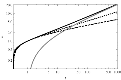
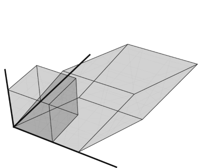
Figure 2: Left panel: Solutions corresponding to the Hamiltonian (10) with the initial conditions $a_{i}\,^{i}(1)=1$, $p^{i}\,_{i}(1)=-1$ (no summation), $a_{i}\,^{j}(1)=0$ $(i\neq j)$, $p^{3}\,_{1}(1)=p^{3}\,_{2}(1)=0$, $p^{2}\,_{1}(1)=0.2$, $\phi(1)=10^{-3}$, $\pi(1)=1.2$. The diagonal momenta $p^{i}\,_{i}$ are chosen to be negative such that all sides of the torus expand. The solid black line is $a_{1}\,^{1}$, the dashed one $a_{2}\,^{2}$, the dotted one $a_{3}\,^{3}$ and the gray one the off-diagonal $a_{2}\,^{1}$. The time $t$ parametrizes the coordinate time in natural units ($c=\kappa=\hbar=1$). Right panel: Solution corresponding to the Hamiltonian (10) at two different times. The initial condition is a cubic universe with $a_{i}\,^{i}\equiv a_{0}$, $p^{i}\,_{i}\equiv p_{0}$, $a_{i}\,^{j}=0$ $(i\neq j)$, $p^{i}\,_{j}\neq 0$ $(i\neq j)$. For both panels the mass and the potential of the scalar field have been set to zero.

We add a matter term consisting of a homogeneous massive scalar field to Equation (2.2) to obtain the Hamiltonian

$$\mathcal{H}=\mathcal{H}_{g}+\mathcal{H}_{\phi}=\mathcal{H}_{g}+\frac{1}{2\sqrt{h}}\pi^{2}+\frac{\sqrt{h}}{2}m_{\phi}^{2}\phi^{2}+\sqrt{h}V(\phi),$$ (10)

where $\pi$ is the momentum of the scalar field, $m_{\phi}$ its mass, $h=(a_{1}\,^{1})^{2}(a_{2}\,^{2})^{2}(a_{3}\,^{3})^{2}$ the determinant of the spatial metric (4) and $V(\phi)$ the potential which we set to zero in the sequel. From this equation we calculate the Friedmann equations and compute the shape of the universe for a special choice of initial conditions, which is shown in Figure 2. All classical solutions have the limit $\lim_{t\rightarrow 0}a_{i}\,^{j}=0$ and grow with $a\propto t^{1/3}$ for a massless scalar field with zero potential. Furthermore, note the convergence of $a_{1}\,^{1}$ and $a_{2}\,^{2}$, which is explained in B.

3 Symmetry Reduction and Classical Phase Space for Ashtekar Variables

In this section we shall repeat the complete analysis introduced in [29, 9, 10] in order to see the role of a compact topology on a connection. Our strategy is to find an invariant connection on the covering space $\tilde{M}$ and then restrict it to the compact space $M$ by means of the covering map (1). In the following section, when referring to the covering space, we shall use a tilde.

3.1 Invariant Connections

Let $\tilde{P}(\tilde{M},SU(2),\pi)$ be a principal fiber bundle over $\tilde{M}$ with structure group $SU(2)$ and projection $\pi:\tilde{P}\rightarrow\tilde{M}$. We require that there be a symmetry group $\tilde{S}\subset\mathrm{Aut}(\tilde{P})$ of bundle automorphisms which acts transitively. Furthermore, for Bianchi I models $\tilde{S}$ does not have a non-trivial isotropy subgroup $\tilde{F}$ so that the base manifold is isomorphic to the symmetry group $\tilde{S}$, i.e. $\tilde{M}/\tilde{S}=\{x_{0}\}$ is represented by a single point that can be chosen arbitrarily in $\tilde{M}$. Since the isotropy group $\tilde{F}$ is trivial the coset space $\tilde{S}/\tilde{F}\cong\tilde{S}$ is reductive with a decomposition of the Lie algebra of $\tilde{S}$ according to $\mathcal{L}\tilde{S}=\mathcal{L}\tilde{F}\oplus\mathcal{L}\tilde{F}_{\perp}=\mathcal{L}\tilde{F}_{\perp}$ together with the trivial condition $\mathrm{Ad}_{\tilde{F}}\mathcal{L}\tilde{F}_{\perp}\subset\mathcal{L}\tilde{F}_{\perp}$. This allows us to use the general framework described in [9, 10, 29].

Since the isotropy group plays an important role in classifying symmetric bundles and invariant connections we describe the general case of a general isotropy group $\tilde{F}$. Fixing a point $x\in\tilde{M}$, the action of $\tilde{F}$ yields a map $\tilde{F}:\pi^{-1}(x)\rightarrow\pi^{-1}(x)$ of the fiber over $x$. To each point $p\in\pi^{-1}(x)$ in the fiber we assign a group homomorphism $\lambda_{p}:\tilde{F}\rightarrow G$ defined by $f(p)=:p\cdot\lambda_{p}(f)$, $\forall f\in\tilde{F}$. As this homomorphism transforms by conjugation $\lambda_{p\cdot g}=\mathrm{Ad}_{g^{-1}}\circ\lambda_{p}$ only the conjugacy class $[\lambda]$ of a given homomorphism matters. In fact, it can be shown [29] that an $\tilde{S}$-symmetric principal bundle $P(\tilde{M},G,\pi)$ with isotropy subgroup $\tilde{F}\subseteq\tilde{S}$ is uniquely characterized by a conjugacy class $[\lambda]$ of homomorphisms $\lambda:\tilde{F}\rightarrow G$ together with a reduced bundle $Q(\tilde{M}/\tilde{S},Z_{G}(\lambda(\tilde{F})),\pi_{Q})$, where $Z_{G}(\lambda(\tilde{F}))$ is the centralizer of $\lambda(\tilde{F})$ in $G$. In our case, since $\tilde{F}=\{1\}$ all homomorphisms $\lambda:\tilde{F}\rightarrow G=SU(2)$ are given by $1\mapsto 1_{G}$.

After having classified the $\tilde{S}$-symmetric fiber bundle $\tilde{P}$ we seek a $[\lambda]$-invariant connection on $\tilde{P}$. We use the following general result [30]:

Theorem 3 (Generalized Wang theorem).

Let $\tilde{P}$ be an $\tilde{S}$-symmetric principal bundle classified by $([\lambda],Q)$ and let $\tilde{\omega}$ be a connection in $\tilde{P}$ which is invariant under the action of $\tilde{S}$. Then $\tilde{\omega}$ is classified by a connection $\tilde{\omega}_{Q}$ in $Q$ and a scalar field (usually called the Higgs field) $\phi:Q\times\mathcal{L}\tilde{F}_{\perp}\rightarrow\mathcal{L}G$ obeying the condition

$$\phi(\mathrm{Ad}_{f}(X))=\mathrm{Ad}_{\lambda(f)}\phi(X),\forall f\in\tilde{F},\;X\in\mathcal{L}\tilde{F}_{\perp}.$$ (11)

The connection $\tilde{\omega}$ can be reconstructed from its classsifying structure as follows. According to the decomposition $\tilde{M}\cong\tilde{M}/\tilde{S}\times\tilde{S}/\tilde{F}$ we have $\tilde{\omega}=\tilde{\omega}_{Q}+\tilde{\omega}_{\tilde{S}/\tilde{F}}$ with $\tilde{\omega}_{\tilde{S}/\tilde{F}}=\phi\circ\iota^{*}\tilde{\theta}_{\mathrm{MC}}$, where $\iota:\tilde{S}/\tilde{F}\hookrightarrow\tilde{S}$ is a local embedding and $\tilde{\theta}_{\mathrm{MC}}$ is the Maurer-Cartan form on $\tilde{S}$. The structure group $G$ acts on $\phi$ by conjugation, whereas the solution space of Equation (11) is only invariant with respect to the reduced structure group $Z_{G}(\lambda(\tilde{F}))$. This fact leads to a partial gauge fixing since the connection form $\tilde{\omega}_{\tilde{S}/\tilde{F}}$ is a $Z_{G}(\lambda(\tilde{F}))$-connection which explicitly depends on $\lambda$. We then break down the structure group from $G$ to $Z_{G}(\lambda(\tilde{F}))$ by fixing a $\lambda\in[\lambda]$.

In our case, the embedding $\iota:\tilde{S}\rightarrow\tilde{S}$ is the identity and the base manifold $\tilde{M}/\tilde{S}=\{x_{0}\}$ of the orbit bundle is represented by a single point so that the invariant connection is given by

$$\tilde{A}=\phi\circ\tilde{\theta}_{\mathrm{MC}}.$$

The three generators of $\mathcal{L}\tilde{S}$ are given by $T_{I}$, $1\leq I\leq 3$, with the relation $[T_{I},T_{J}]=0$ for Bianchi I models. The Maurer-Cartan form is given by $\tilde{\theta}_{\mathrm{MC}}=\tilde{\omega}^{I}T_{I}$ where $\tilde{\omega}^{I}$ are the left invariant one-forms on $\tilde{S}$. The condition (11) is empty so that the Higgs field is given by $\phi:\mathcal{L}\tilde{S}\rightarrow\mathcal{L}G,\;T_{I}\mapsto\phi(T_{I})=:\phi_{I}\,^{i}\tau_{i}$, where the matrices $\tau_{j}=-i\sigma_{j}/2$, $1\leq j\leq 3$, generate $\mathcal{L}G$, where $\sigma_{j}$ are the standard Pauli matrices. In summary the invariant connection is given by

$$\tilde{A}=\phi_{I}\,^{i}\tau_{i}d\tilde{\omega}^{I}.$$ (12)

In order to restrict this invariant connection we define the invariant connection $A$ on $\mathds{T}^{3}$ with the pullback given by the covering map (1). The generators of the Teichmüller space (see Equation (2)) allow us to write $A$ as:

$$A_{a}^{i}:=\bar{\phi}_{I}\,^{i}\omega_{a}^{I},\quad(\bar{\phi}_{I}\,^{i})=\left(\begin{array}[]{ccc}\bar{\phi}_{1}\,^{1}&\bar{\phi}_{2}\,^{1}&\bar{\phi}_{3}\,^{1}\\ 0&\bar{\phi}_{2}\,^{2}&\bar{\phi}_{3}\,^{2}\\ 0&0&\bar{\phi}_{3}\,^{3}\end{array}\right).$$ (13)

3.1.1 Simplified Model

In the sequel we shall concentrate on a simpler model for which we can also easily satisfy the Gauss constraint. We choose a torus generated by the vectors $a_{1}=(a_{1}\,^{1},0,0)^{T}$, $a_{2}=(0,a_{2}\,^{2},a_{2}\,^{3})^{T}$ and $a_{3}=(0,a_{3}\,^{2},a_{3}\,^{3})^{T}$ (see Figure 3) such that

$$(\bar{\phi}_{I}\,^{i})=\left(\begin{array}[]{ccc}\bar{\phi}_{1}\,^{1}&0&0\\ 0&\bar{\phi}_{2}\,^{2}&\bar{\phi}_{3}\,^{2}\\ 0&\bar{\phi}_{2}\,^{3}&\bar{\phi}_{3}\,^{3}\end{array}\right),\quad(\omega_{a}^{I})=\left(\begin{array}[]{ccc}a_{1}\,^{1}&0&0\\ 0&a_{2}\,^{2}&a_{3}\,^{2}\\ 0&a_{2}\,^{3}&a_{3}\,^{3}\end{array}\right)$$ (14)

and

$$(A_{a}^{i})=\left(\begin{array}[]{ccc}a_{1}\,^{1}\bar{\phi}_{1}\,^{1}&0&0\\ 0&a_{2}\,^{2}\bar{\phi}_{2}\,^{2}+a_{2}\,^{3}\bar{\phi}_{3}\,^{2}&a_{3}\,^{2}\bar{\phi}_{2}\,^{2}+a_{3}\,^{3}\bar{\phi}_{3}\,^{2}\\ 0&a_{2}\,^{2}\bar{\phi}_{2}\,^{3}+a_{2}\,^{3}\bar{\phi}_{3}\,^{3}&a_{3}\,^{2}\bar{\phi}_{2}\,^{3}+a_{3}\,^{3}\bar{\phi}_{3}\,^{3}\end{array}\right)$$

The vectors $X_{I}$ dual to $\omega^{I}$ are given by

$$X_{1}=\left(\begin{array}[]{c}\frac{1}{a_{1}\,^{1}}\\ 0\\ 0\end{array}\right),\;X_{2}=\frac{1}{\mathfrak{h}}\left(\begin{array}[]{c}0\\ a_{3}\,^{3}\\ -a_{2}\,^{3}\end{array}\right),\;X_{3}=\frac{1}{\mathfrak{h}}\left(\begin{array}[]{c}0\\ -a_{3}\,^{2}\\ a_{2}\,^{2}\end{array}\right),$$

where we defined $\mathfrak{h}=a_{2}\,^{2}a_{3}\,^{3}-a_{2}\,^{3}a_{3}\,^{2}$.

Figure 3: The vectors $a_{1}$, $a_{2}$ and $a_{3}$ span the torus with five Teichmüller parameters. The vectors $a_{2}$ and $a_{3}$ lie in the $\xi_{2}\xi_{3}$-plane while $a_{1}$ is aligned with $\xi_{1}$

3.2 Classical Phase Space for Ashtekar Variables

The phase space of full general relativity in the Ashtekar representation is spanned by the $SU(2)$-connection $A_{a}^{i}=\Gamma_{a}^{i}+\gamma K_{a}^{i}$ and the densitized triad $E_{i}^{a}=|\det e|e_{i}^{a}$, where $\Gamma_{a}^{i}$ is the spin connection, $K_{a}^{i}$ the extrinsic curvature, $e_{i}^{a}$ the triad and $\gamma>0$ the Immirzi parameter [17, 18, 19]. The symplectic stucture of full general relativity is given by the Poisson bracket

$$\{A^{i}_{a}(y),E^{b}_{j}(x)\}=\kappa\delta_{a}^{b}\delta_{j}^{i}\delta(x,y).$$ (15)

The connection between the metric and the densitized triad is given by

$$hh^{ab}=\delta^{ij}E_{i}^{a}E_{j}^{b},$$ (16)

where $h^{ab}$ is the inverse of the metric $h_{ab}$.

We can now use the results obtained in Section 2 to construct the phase space $\mathcal{P}$ in this representation. In the preceding subsection we have already found the configuration space is spanned by $\bar{\phi}_{I}\,^{i}$ (see Equation (14)). On the other hand, the densitized triad dual to the connection is given by

$$(E^{a}_{i})=\sqrt{h}\bar{p}^{I}\,_{i}X^{a}_{I}=\sqrt{h}\left(\begin{array}[]{ccc}\frac{\bar{p}^{1}\,_{1}}{a_{1}\,^{1}}&0&0\\ 0&\frac{a_{3}\,^{3}\bar{p}^{2}\,_{2}-a_{3}\,^{2}\bar{p}^{3}\,_{2}}{\mathfrak{h}}&\frac{a_{3}\,^{3}\bar{p}^{2}\,_{3}-a_{3}\,^{2}\bar{p}^{3}\,_{3}}{\mathfrak{h}}\\ 0&\frac{a_{2}\,^{2}\bar{p}^{3}\,_{2}-a_{2}\,^{3}\bar{p}^{2}\,_{2}}{\mathfrak{h}}&\frac{a_{2}\,^{2}\bar{p}^{3}\,_{3}-a_{2}\,^{3}\bar{p}^{2}\,_{3}}{\mathfrak{h}}\end{array}\right),$$ (17)

where

$$(\bar{p}^{I}\,_{i})=\left(\begin{array}[]{ccc}\bar{p}^{1}\,_{1}&0&0\\ 0&\bar{p}^{2}\,_{2}&\bar{p}^{2}\,_{3}\\ 0&\bar{p}^{3}\,_{2}&\bar{p}^{3}\,_{3}\end{array}\right),$$

together with $\omega_{a}^{J}X^{a}_{I}=\delta^{J}_{I}$ and $h=(a_{1}\,^{1})^{2}(a_{2}\,^{3}a_{3}\,^{2}-a_{2}\,^{2}a_{3}\,^{3})^{2}$ is the determinant of the spatial metric constructed from the vectors $a_{i}$ and $\bar{p}^{I}\,_{i}$ the momentum dual to $\bar{\phi}_{I}\,^{i}$ satisfying the Poisson bracket

$$\{\bar{\phi}_{I}\,^{i},\bar{p}^{J}\,_{j}\}=\frac{\kappa\gamma}{V_{0}}\delta_{I}^{J}\delta_{j}^{i}$$ (18)

with the volume $V_{0}=\int_{\mathds{T}^{3}}d^{3}x\sqrt{h}$ of $\mathds{T}^{3}$ as measured by the metric $h$. For later purpose we define new variables

$$\phi_{I}\,^{i}=L_{I}\bar{\phi}_{I}\,^{i},\quad p^{I}\,_{i}=\frac{V_{0}}{L_{I}}\bar{p}^{I}\,_{i},$$ (19)

such that

$$\{\phi_{I}\,^{i},p^{J}\,_{j}\}=\kappa\gamma\delta_{I}^{J}\delta_{j}^{i},$$ (20)

where

$$L_{1}=a_{1}\,^{1},\;L_{2}=\sqrt{(a_{2}\,^{2})^{2}+(a_{2}\,^{3})^{2}},\;L_{3}=\sqrt{(a_{3}\,^{2})^{2}+(a_{3}\,^{3})^{2}}.$$

Thus we conclude that

Proposition 1.

The classical configuration space $\mathcal{A}_{S}=\mathds{R}^{5}$ is spanned by the five configuration variables $\phi_{I}\,^{i}$. The phase space $\mathcal{P}=\mathds{R}^{10}$ is spanned by $\phi_{I}\,^{i}$ and the five momenta $p^{J}\,_{j}$ satisfying the Poisson bracket (20).

Furthermore, note that the determinant of the densitized triad is given by

$$\det E_{i}^{a}=\mathfrak{k}\,p^{1}\,_{1}(p^{2}\,_{3}p^{3}\,_{2}-p^{2}\,_{2}p^{3}\,_{3}),$$ (21)

where we defined

$$\mathfrak{k}:=\frac{L_{1}L_{2}L_{3}}{V_{0}}.$$

The relation between the new variables $(\phi_{I}\,^{i},p^{J}\,_{j})$ and the ’scale factors’ $a_{a}\,^{b}$ and their respective momenta $p^{a}\,_{b}$ can be found by using Equation (16) and the Poisson brackets (7) and (20). A closed form could only be found for $p^{1}\,_{1}$ and is given by

$$|p^{1}\,_{1}|=|a_{2}\,^{2}a_{3}\,^{3}-a_{2}\,^{3}a_{3}\,^{2}|.$$

3.3 Constraints in Ashtekar Variables on the Torus

In the canonical variables (15) the Legendre transform of the Einstein-Hilbert action (5) results in a fully constrained system [17, 18, 19]

$$S=\frac{1}{2\kappa}\int_{\mathds{R}}dt\int_{\mathds{T}^{3}}d^{3}x\left(2\dot{A}_{a}^{i}E^{a}_{i}-[\Lambda^{j}G_{j}+N^{a}H_{a}+N\mathcal{H}]\right),$$ (22)

where $G_{j}$ is the Gauss constraint, $H_{a}$ the diffeomorphism (or vector) constraint, $\mathcal{H}$ the Hamiltonian and $\Lambda^{j}$, $N^{a}$, $N$ are Lagrange multipliers. The Hamiltonian constraint simplifies to

$$C_{\mathrm{grav}}=-\frac{1}{2\kappa}\int_{\mathds{T}^{3}}d^{3}xN\epsilon_{ijk}F^{i}_{ab}\frac{E^{aj}E^{bk}}{\sqrt{|\mathrm{det}E|}}$$ (23)

due to spatial flatness, where the curvature of the Ashtekar connection is given by

$$F_{ab}^{i}=\partial_{a}A_{b}^{i}-\partial_{b}A_{a}^{i}+\epsilon^{i}_{jk}A^{j}_{a}A^{k}_{b}=\epsilon^{i}_{jk}A^{j}_{a}A^{k}_{b}.$$

Homogeneity further requires that $N\neq N(x)$. Inserting Equation (14) and Equation (17) into Equation (23) we get

$$C_{\mathrm{grav}}= -\frac{1}{\kappa\gamma^{2}}\frac{1}{\sqrt{|p^{1}\,_{1}(p^{2}\,_{2}p^{3}\,_{3}-p^{2}\,_{3}p^{3}\,_{2})|}}\times$$ (24)

$$\Bigl{[} \phi_{1}\,^{1}p^{1}\,_{1}\left\{(\phi_{2}\,^{2}-\phi_{2}\,^{3})(p^{2}\,_{2}-p^{2}\,_{3})+(\phi_{3}\,^{2}-\phi_{3}\,^{3})(p^{3}\,_{2}-p^{3}\,_{3})\right\}$$

$$+(\phi_{2}\,^{3}\phi_{3}\,^{2}-\phi_{2}\,^{2}\phi_{3}\,^{3})(p^{2}\,_{3}p^{3}\,_{2}-p^{2}\,_{2}p^{3}\,_{3})\Bigr{]},$$

where we defined $N=\sqrt{L_{1}L_{2}L_{3}/V_{0}}$ in order to simplify the Hamiltonian. Using the Hamiltonian (24) we can compute the time evolution of the basic variables $\phi_{i}\,^{j}$ and $p^{i}\,_{j}$ (see Figure 4). Setting all off-diagonal terms to zero we see that Equation (24) matches with Eq. (3.20) in [31]. If we further set $\phi_{(i)}\,^{i}=c$ and $p^{(i)}\,_{i}=p$ we get

$$C_{\mathrm{grav}}=-\frac{3}{\kappa\gamma^{2}}c^{2}\sqrt{|p|},$$

which is exactly the same result as the homogeneous and isotropic case [8].

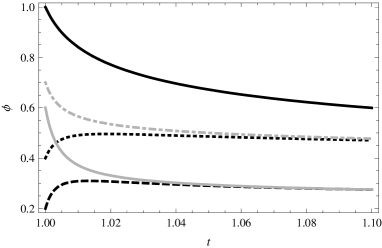
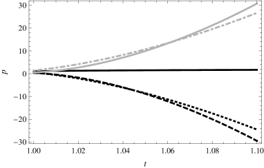
Figure 4: Solutions corresponding to the Hamiltonian (24) coupled to a massless scalar field with vanishing potential. Left panel: the black thick solid shows the evolution of $\phi_{1}\,^{1}$, $\phi_{2}\,^{2}$ is the black dashed line, $\phi_{3}\,^{3}$ the dotted line, $\phi_{2}\,^{3}$ the gray dashdotted one and $\phi_{3}\,^{2}$ the solid gray one. Right panel: the black thick solid shows the evolution of $p^{1}\,_{1}$, $p^{2}\,_{2}$ is the black dashed line, $p^{3}\,_{3}$ the dotted line, $p^{2}\,_{3}$ the gray dashdotted one and $p^{3}\,_{2}$ the solid gray one. In both cases the initial conditions are $\phi_{1}\,^{1}=1.0$, $\phi_{2}\,^{2}=0.2$, $\phi_{3}\,^{3}=0.4$, $\phi_{2}\,^{3}=0.6$, $\phi_{3}\,^{2}=0.7$, $p^{1}\,_{1}=1.0$, $p^{2}\,_{2}=0.3$, $p^{3}\,_{3}=0.5$, $p^{2}\,_{3}0.5$, $p^{3}\,_{2}=1.4$, $\phi=0.01$ and $p_{\phi}=8.1$. The time $t$ parametrizes the coordinate time in natural units ($c=\kappa=\hbar=1$).

3.4 Diffeomeorphism and Gauss Constraints

The Gauss constraint stems from the fact that we chose the densitized triads $E_{i}^{a}$ as the momenta conjugated to the connections $A_{a}^{i}$. In fact, the spacial metric can be directly obtained from the densitized triads through Equation (16) and is invariant under rotations given by $E_{i}^{a}\mapsto O_{i}^{j}E_{j}^{a}$. In order that the theory be invariant under such rotations the Gauss constraint

$$G_{i}=\partial_{a}E^{a}_{i}+\epsilon_{ijk}A^{j}_{a}E^{a}_{k}\approx 0$$ (25)

must be satisfied. The diffeomorphism constraint modulo Gauss constraint originates from the requirement of independence from any spatial coordinate system or background and is given by

$$H_{a}=F^{i}_{ab}E^{b}_{i}\approx 0.$$ (26)

However, as mentioned in [21] we have to be careful when dealing with these constraints in the case where the topology is closed. We thus divide this subsection into two parts, starting with the general case of open models.

3.4.1 Open Models

Due to spatial homogeneity of Bianchi type I models the basic variables can be diagonalized to [9, 14]

$$A^{{}^{\prime}i}_{a}=\tilde{c}^{\prime}_{(K)}\Lambda^{{}^{\prime}i}_{K}\omega^{{}^{\prime}K}_{a},\quad E^{{}^{\prime}a}_{i}=p^{{}^{\prime}(K)}\Lambda^{{}^{\prime}K}_{i}X^{{}^{\prime}a}_{K},$$

where $\omega^{\prime}$ is the left-invariant 1-form, $X^{\prime}$ the densitized left-invariant vector field dual to $\omega^{\prime}$ and $\Lambda^{\prime}\in SO(3)$. This choice of variables automatically satisfies the vector and Gauss constraints, thus reducing the analysis of Equation (22) to the Hamiltonian constraint (23). The homogeneous, anisotropic vacuum solution to the Einstein field equations is called the Kasner solution and is given by the following metric:

$$ds^{2}=-d\tau^{2}+\tau^{2\alpha_{1}}dx_{1}^{2}+\tau^{2\alpha_{2}}dx_{2}^{2}+\tau^{2\alpha_{3}}dx_{3}^{2}$$

where the two constraints $\alpha_{i}\in\mathds{R}$, $\sum\alpha_{i}=\sum\alpha_{i}^{2}=1$ have to be fulfilled. These imply that not all Kasner exponents can be equal, i.e. isotropic expansion or contraction of space is not allowed. By contrast the RW metric is able to expand or contract isotropically because of the presence of matter. At the end, from the twelve-dimensional phase space only two degrees of freedom remains.

An infinitesimal diffeomorphism generated by a vector field $V$ induces the following action on the left-invariant 1-form $\omega^{\prime}$:

$$\omega_{a}\mapsto\omega^{\prime}_{a}+\epsilon\mathcal{L}_{V}\omega^{\prime}_{a},$$ (27)

where $\mathcal{L}_{V}$ is the Lie derivative along $V$. Such transformations leave the metric homogeneous provided the vector fields satisfy

$$V^{a}=-(f_{j}^{i}y^{j})X^{{}^{\prime}a}_{i}$$ (28)

for some constants $f_{j}^{i}$ and functions $y^{i}$ given by $\mathcal{L}_{K_{j}}y^{i}=\delta_{j}^{i}$ [21]. The last equation for $y^{i}$ relies on the fact that the 3-surface is topologically $\mathds{R}^{3}$ and the Killing vectors $K_{i}$ commute. As we shall see below this will not be the case in the closed models.

In the case of rotational symmetry the diffeomorphism constraint is once again satisfied by the choice of variables whereas the Gauss constraint is not. However, in such a case the triad components can be rotated until the Gauss constraint is also satisfied. Further details can be found in [32].

3.4.2 The Torus as a Closed Model

As we have seen in Section 2 it is not possible to align the Killing fields with the left-invariant vectors, whence the metric takes the non-diagonal form (4) and the Ashtekar connection the form (13). In the previous subsection we saw that a diffeomorphism preserves homogeneity provided it satisfies the condition (28). In the closed model the analysis goes through as well and we find that $V_{i}$ has to satisfy the same condition (28). However, since such fields lack the required periodicity in $x^{i}$ we are led to the conclusion that there are no globally defined, non-trivial homogeneity preserving diffeomorphisms (HPDs) and there is no analog of (27). Thus, instead of one degree of freedom we get additional degrees of freedom.

The Gauss constraint for a Bianchi type I model is given by

$$G_{i}=\epsilon_{ijk}\phi_{I}\,^{i}p^{I}\,_{k}.$$ (29)

With our choice of variables two Gauss constraints are automatically satisfied, namely $G_{2}=G_{3}\equiv 0$. However, we can still perform a global $SU(2)$ transformation along $\tau_{1}$ which is implemented in the nonvanishing Gauss constraint

$$G_{1}=\phi_{2}\,^{2}p^{2}\,_{3}+\phi_{3}\,^{2}p^{3}\,_{3}-\phi_{2}\,^{3}p^{2}\,_{2}-\phi_{3}\,^{3}p^{3}\,_{2}\approx 0$$ (30)

generating simultaneous rotations of the pairs $(\phi_{2}\,^{2},\phi_{2}\,^{3})$, $(p^{2}\,_{2},p^{2}\,_{3})$ resp. $(\phi_{3}\,^{2},\phi_{3}\,^{3})$, $(p^{3}\,_{2},p^{3}\,_{3})$. Thus the norms of these vectors and the scalar products between them are gauge invariant. The Gauss constraint allows us to get rid of e.g. the pair $(\phi_{3}\,^{2},p^{3}\,_{2})$ by fixing the gauge in the following way: we rotate the connection components such that $\phi_{3}\,^{2}=0$. Because the length $\|\phi_{3}\|=\sqrt{(\phi_{3}\,^{2})^{2}+(\phi_{3}\,^{3})^{2}}$ is preserved we know that $\phi_{3}\,^{3}\neq 0$. The Gauss constraint then implies that $p^{3}\,_{2}=(\phi_{2}\,^{2}p^{2}\,_{3}-\phi_{2}\,^{3}p^{2}\,_{2})/\phi_{3}\,^{3}$. This gauge fixing reduces the degrees of freedom by two units.

The diffeomorphism constraint is given by Equation (26) and since $F_{ab}^{i}=\epsilon^{i}\,_{jk}A_{a}^{j}A_{b}^{k}$ ($\partial_{a}A_{b}^{i}=0$ thanks to homogeneity) we find that

$$H_{a}=\epsilon^{i}\,_{jk}A_{a}^{j}A_{b}^{k}E^{b}_{i}\propto A^{i}_{a}G_{i}.$$ (31)

The gauge fixing we just performed ensures that the diffeomorphism constraint also vanishes.

3.5 Canonical Transformation

In this subsection we introduce a set of new variables which will greatly simplify the analysis of the kinematical Hilbert space. We first perform a canonical transformation on the unreduced phase space:

$$Q_{1}=\phi_{1}\,^{1},\quad P^{1}=p^{1}\,_{1},$$

$$Q_{2}=\sqrt{(\phi_{2}\,^{2})^{2}+(\phi_{2}\,^{3})^{2}},\quad P^{2}=\frac{p^{2}\,_{2}\phi_{2}\,^{2}+p^{2}\,_{3}\phi_{2}\,^{3}}{\sqrt{(\phi_{2}\,^{2})^{2}+(\phi_{2}\,^{3})^{2}}}$$

$$Q_{3}=\sqrt{(\phi_{3}\,^{2})^{2}+(\phi_{3}\,^{3})^{2}},\quad P^{3}=\frac{p^{3}\,_{2}\phi_{3}\,^{2}+p^{3}\,_{3}\phi_{3}\,^{3}}{\sqrt{(\phi_{3}\,^{2})^{2}+(\phi_{3}\,^{3})^{2}}}$$ (32)

$$\theta_{1}=\mathrm{arc}_{k}\mathrm{cos}\left(\frac{\phi_{2}\,^{2}}{\sqrt{(\phi_{2}\,^{2})^{2}+(\phi_{2}\,^{3})^{2}}}\right),\quad P_{\theta_{1}}=p^{2}\,_{3}\phi_{2}\,^{2}-p^{2}\,_{2}\phi_{2}\,^{3}$$

$$\theta_{2}=\mathrm{arc}_{k}\mathrm{cos}\left(\frac{\phi_{3}\,^{3}}{\sqrt{(\phi_{3}\,^{2})^{2}+(\phi_{3}\,^{3})^{2}}}\right),\quad P_{\theta_{2}}=-p^{3}\,_{3}\phi_{3}\,^{2}+p^{3}\,_{2}\phi_{3}\,^{3}$$

such that the variables are mutually conjugate:

$$\{Q_{I},P^{J}\}=\frac{\kappa\gamma}{V_{0}}\delta_{I}^{J},\quad\{\theta_{\alpha},P_{\theta_{\beta}}\}=\frac{\kappa\gamma}{V_{0}}\delta_{\alpha,\beta}.$$

We choose the convention that the diagonal limit can be recovered by setting $\theta_{1}=\theta_{2}=0$. The inverse of this canonical transformation will be important in the sequel and is given by:

$$\phi_{2}\,^{2}=Q_{2}\cos(\theta_{1}),\quad \phi_{2}\,^{3}=Q_{2}\sin(\theta_{1}),$$

$$p^{2}\,_{2}=P^{2}\cos(\theta_{1})-\frac{P_{\theta_{1}}\sin(\theta_{1})}{Q_{2}},\quad p^{2}\,_{3}=\frac{P_{\theta_{1}}\cos(\theta_{1})}{Q_{2}}+P^{2}\sin(\theta_{1}),$$ (33)

$$\phi_{3}\,^{2}=Q_{3}\sin(\theta_{2}),\quad \phi_{3}\,^{3}=Q_{3}\cos(\theta_{2}),$$

$$p^{3}\,_{2}=P^{3}\sin(\theta_{2})+\frac{P_{\theta_{2}}\cos(\theta_{2})}{Q_{3}},\quad p^{3}\,_{3}=-\frac{P_{\theta_{2}}\sin(\theta_{2})}{Q_{3}}+P^{3}\cos(\theta_{2}).$$

It is important to note that $Q_{2},Q_{3}\in\mathds{R}_{+}$ and $\theta_{1},\theta_{2}\in[k\pi,(k+1)\pi]$ where we restrict the values of $k$ to be either $k=0$ if $\mathrm{sgn}(\phi_{2}\,^{3})>0$ or $k=1$ if $\mathrm{sgn}(\phi_{2}\,^{3})<0$. If $\mathrm{sgn}(\phi_{2}\,^{3})=0$ then we have the case $k=0$ if $\mathrm{sgn}(\phi_{2}\,^{2})>0$ or $k=1$ if $\mathrm{sgn}(\phi_{2}\,^{2})<0$. The function arc₁cos$(x)$ is related to the principal value via arc₁cos$(x)=2\pi-$arccos$(x)$. With this convention we can recover Equation (3.5) unambiguiously from Equation (3.5).

The Hamiltonian constraint (24) is given in terms of the new variables by

$$C_{\mathrm{grav}}=\frac{(2\kappa\gamma^{2})^{-1}}{\sqrt{\left|\frac{P^{1}\left[\cos(\theta_{1}+\theta_{2})(P_{\theta_{1}}P_{\theta_{2}}-P^{2}P^{3}Q_{2}Q_{3})+(P^{2}P_{\theta_{2}}Q_{2}+P^{3}P_{\theta_{1}}Q_{3})\sin(\theta_{1}+\theta_{2})\right]}{Q_{2}Q_{3}}\right|}}\times$$

$$\times\biggl{\{}2P^{1}Q_{1}\Bigl{[}\cos(2\theta_{2})P_{\theta_{2}}+P^{2}Q_{2}(\sin(2\theta_{1})-1)+P^{3}Q_{3}(\sin(2\theta_{2})-1)\Bigr{]}$$

$$\quad\;\;+P^{2}Q_{2}\Bigl{[}P_{\theta_{2}}\sin(2(\theta_{1}+\theta_{2}))-2\cos^{2}(\theta_{1}+\theta_{2})P^{3}Q_{3}\Bigr{]}$$ (34)

$$\quad\;\;+P_{\theta_{1}}\Bigl{[}2\cos^{2}(\theta_{1}+\theta_{2})P_{\theta_{2}}+2\cos(2\theta_{1})P^{1}Q_{1}+P^{3}P_{\theta_{3}}\sin(2(\theta_{1}+\theta_{2}))\Bigr{]}\biggl{\}}$$

Using this Hamiltonian we can compute the time evolution of the basic variables $Q_{i}$, $\theta_{\alpha}$, $P^{i}$ and $P_{\theta_{\alpha}}$ (see Figure 5). We choose the initial conditions so that they correspond to the values of the old variables (see caption of Figure 4). By doing so we are able to check whether the solutions to Equation (24) are equivalent to the solutions to Equation (3.5) by performing the canonical transformation (3.5). The different solutions do indeed match up to a very good accuracy.

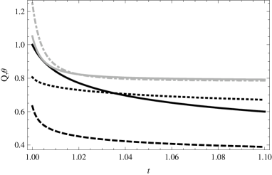
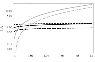
Figure 5: Solutions corresponding to the Hamiltonian (3.5) coupled to a massless scalar field with vanishing potential. Left panel: the black thick solid shows the evolution of $Q_{1}$, $Q_{2}$ is the black dashed line, $Q_{3}$ the dotted line, $\theta_{1}$ the gray dashdotted one and $\theta_{2}$ the solid gray one. Right panel: the black thick solid shows the evolution of $P^{1}$, $P^{2}$ is the black dashed line, $P^{3}$ the dotted line, $P_{\theta_{1}}$ the gray dashdotted one and $P_{\theta_{2}}$ the solid gray one. In both cases the initial conditions are $Q_{1}=1$, $Q_{2}=0.63$, $Q_{3}=0.81$, $\theta_{1}=1.25$, $\theta_{2}=1.05$, $P^{1}=1$, $P^{2}=0.57$, $P^{3}=1.46$, $P_{\theta_{1}}=-0.08$, $P_{\theta_{2}}=0.21$, $\phi=0.01$ and $p_{\phi}=8.1$. The time $t$ parametrizes the coordinate time in natural units ($c=\kappa=\hbar=1$).

The only nontrivial Gauss constraint (30) is then given by

$$G_{1}=P_{\theta_{1}}-P_{\theta_{2}},$$ (35)

which vanishes only when $P_{\theta_{2}}=P_{\theta_{1}}$. We are free to fix the gauge by setting $\theta_{2}=0$. The same result can be obtained from the gauge fixing performed in Section 3.4.2 so that

$$Q_{3}=\phi_{3}\,^{3},\quad P^{3}=p^{3}\,_{3},\quad\theta_{2}=0\quad\mathrm{and}\quad P_{\theta_{2}}=P_{\theta_{1}}.$$

The symplectic structure of the reduced 8-dimensional phase space is given by

$$\mathbf{\Omega}=\frac{V_{0}}{\kappa\gamma}(dQ_{1}\wedge dP^{1}+dQ_{2}\wedge dP^{2}+dQ_{3}\wedge dP^{3}+d\theta_{1}\wedge dP_{\theta_{1}}).$$

4 Kinematical Hilbert Space

4.1 Holonomies

In the last section we parametrized the classical phase space and gave the Hamiltonian in terms of the Ashtekar variables. To quantize the theory we have to select a set of elementary observables which have unambiguous operator analogs. In order to do so we have first to find elementary variables of the 5-dimensional configuration space.

According to [10] the configuration space on the covering space $\tilde{\Sigma}$ is given by Higgs fields in a single point $x_{0}$ which is the only point in the reduced manifold $\tilde{\Sigma}/\tilde{S}$. In quantum theory these fields are represented as point holonomies associated to the point $x_{0}$ [33]. On $\tilde{S}$ we can take the three edges $\xi_{1}$, $\xi_{2}$ and $\xi_{3}$ in order to regularize the point holonomies. However, we would like to apply this construction to a closed manifold. First we note that $\Sigma\cong\tilde{S}/\Gamma$ such that two elements $g,g^{\prime}\in\tilde{S}$ are equivalent if there is an element $\gamma\in\Gamma$ such that $g^{\prime}=g+\gamma$. We can thus restrict the regularization of the point holomonies to the three edges $X_{1}$, $X_{2}$ and $X_{3}$ meeting at $x_{0}$ without losing information. Our elementary configuration variables are then the holonomies along straight lines $\gamma_{I}:[0,1]\rightarrow\Sigma$ defined by the connection $A\propto(\phi_{I}\,^{i})$ [10, 11, 12, 13, 14]. Now the holonomies along $X_{1}$, $X_{2}$ resp. $X_{3}$ are given by

$$h_{1}^{(\lambda_{1})} = \exp(\lambda_{1}\phi_{1}\,^{1}\tau_{1})=\cos(\lambda_{1}\phi_{1}\,^{1})+2\tau_{1}\sin(\lambda_{1}\phi_{1}\,^{1})$$

$$h_{2}^{(\lambda_{2})} = \exp(\lambda_{2}\phi_{2}\,^{2}\tau_{2}+\lambda_{2}\phi_{2}\,^{3}\tau_{3})$$ (36)

$$h_{3}^{(\lambda_{3})} = \exp(\lambda_{3}\phi_{3}\,^{2}\tau_{2}+\lambda_{3}\phi_{3}\,^{3}\tau_{3}),$$

where $\lambda_{I}\in(-\infty,\infty)$ and $\lambda_{I}L_{I}$ is the length of the edge $I$ with respect to the spatial metric $h_{ab}$. The auxilary Hilbert space is then generated by spin networks associated with graphs consisting of the three edges $\gamma_{I}$ meeting at the vertex $x_{0}$.

In open Bianchi type I models the gauge invariant information of the connection can be separated from the gauge degrees of freedom via the relation $\phi_{I}^{i}=c_{(I)}\Lambda_{I}^{i}$ with $\Lambda\in SO(3)$ so that the holonomies become simple trigonometric functions. In our case the situation is more complicated because the holonomies $h_{2}$ and $h_{3}$ cannot be reduced to such functions since

$$h_{\alpha}^{(\lambda_{\alpha})}=\cos\left(\lambda_{\alpha}\|\vec{\phi}_{\alpha}\|/2\right)+2\frac{\phi_{\alpha}\,^{i}\tau_{i}}{\|\vec{\phi}_{\alpha}\|}\sin\left(\lambda_{\alpha}\|\vec{\phi}_{\alpha}\|/2\right)\quad(\mathrm{no}\;\mathrm{summation}),$$

where $\alpha=2,3$ and

$$\|\vec{\phi}_{\alpha}\|:=\sqrt{\sum_{i}(\phi_{\alpha}\,^{i})^{2}}.$$

The problem is that this expression cannot be used in this form since there is no well defined operator $\hat{\phi}_{I}\,^{i}$ on the kinematical Hilbert space. Using the canonical transformation (3.5) we can re-express the holonomies such that

$$h_{1}^{(\lambda_{1})}=\cos(\lambda_{1}Q_{1}/2)+2\tau_{1}\sin(\lambda_{1}Q_{1}/2),$$

$$h_{2}^{(\lambda_{2})}=\cos(\lambda_{2}Q_{2}/2)+2(\tau_{2}\cos\theta_{1}+\tau_{3}\sin\theta_{1})\sin(\lambda_{2}Q_{2}/2),$$ (37)

$$h_{3}^{(\lambda_{3})}=\cos(\lambda_{3}Q_{3}/2)+2(\tau_{2}\sin\theta_{2}+\tau_{3}\cos\theta_{2})\sin(\lambda_{3}Q_{3}/2).$$

Since $\lambda_{I}\in\mathds{R}$ matrix elements of the exponentials of $Q_{1}$, $Q_{2}$ and $Q_{3}$ form a $C^{*}$-algebra of almost periodic functions. On the other hand the variables $\theta_{1,2}$ are periodic angles such that only strictly periodic functions $\exp(ik_{\alpha}\theta_{\alpha})\in U(1)$ with $k_{\alpha}\in\mathds{Z}$ are allowed. Thus, any function generated by this set can be written as

$$g(Q_{1},Q_{2},Q_{3},\theta_{1},\theta_{2})=\sum_{\lambda_{1},\lambda_{2},\lambda_{3},k_{1},k_{2}}\xi_{\lambda_{1},\lambda_{2},\lambda_{3},k_{1},k_{2}}\times$$

$$\quad\quad\times\exp\left(\frac{1}{2}i\lambda_{1}Q_{1}+\frac{1}{2}i\lambda_{2}Q_{2}+\frac{1}{2}i\lambda_{3}Q_{3}+ik_{1}\theta_{1}+ik_{2}\theta_{2}\right)$$ (38)

with coefficients $\xi_{\lambda_{1},\lambda_{2},\lambda_{3},k_{1},k_{2}}\in\mathds{C}$, generating the $C^{*}$-algebra $\mathcal{A}_{S}$. Note that this function is almost periodic in $Q_{1}$,$Q_{2}$ and $Q_{3}$ and strictly periodic in $\theta_{1}$ and $\theta_{2}$. The spectrum of the algebra of the almost periodic functions is called the Bohr compactification $\bar{\mathds{R}}_{B}:=\Delta(\mathrm{Cyl}_{S})$ of the real line and can be seen as the space of generalized connections [13, 34]. Thus the functions (4.1) provide us a complete set of continuous functions on $\bar{\mathds{R}}_{B}\times\bar{\mathds{R}}_{B}\times\bar{\mathds{R}}_{B}\times S^{1}\times S^{1}$. Moreover the Gel’fand theory guarantees that the space $\bar{\mathds{R}}_{B}$ is compact and Hausdorff [35] with a unique normalized Haar measure $d\mu(c)$ such that

$$\int f(c)d\mu(c):=\lim_{T\rightarrow\infty}\frac{1}{2T}\int_{-T}^{T}f(c)dc.$$

A Cauchy completion leads to a Hilbert space $\mathcal{H}^{S}$ defined by the tensor product $\mathcal{H}^{S}=\mathcal{H}_{B}^{\otimes 3}\otimes\mathcal{H}_{S^{1}}^{\otimes 2}$ with the Hilbert spaces $\mathcal{H}_{B}=L^{2}(\bar{\mathds{R}}_{B},d\mu(c))$ and $\mathcal{H}_{S^{1}}=L^{2}(S^{1},d\phi)$ of square integrable functions on $\bar{\mathds{R}}_{B}$ and the circle respectively, where $d\phi$ is the Haar measure for $S^{1}$. An orthonormal basis for $\mathcal{H}_{B}$ is given by the almost periodic functions $\langle Q_{I}|\mu_{I}\rangle=\exp(i\mu_{I}Q_{I}/2)$ (no summation) with $\mu_{I}\in\mathds{R}$ with $\langle\mu_{I}|\mu_{I}^{\prime}\rangle=\delta_{\mu_{I},\mu_{I}^{\prime}}$. Analogously a basis for $\mathcal{H}_{S^{1}}$ is given by the strictly periodic functions $\langle\theta_{\alpha}|k_{\alpha}\rangle=\exp(ik_{\alpha}\theta_{\alpha})$ with $\langle k_{\alpha}|k^{\prime}_{\alpha}\rangle=\delta_{k_{\alpha},k^{\prime}_{\alpha}}$.

We choose a representation where the configuration variables, now promoted to operators, act by multiplication via:

$$(\hat{g}_{1}g_{2})(\vec{Q},\vec{\theta})=g_{1}(\vec{Q},\vec{\theta})g_{2}(\vec{Q},\vec{\theta}).$$

The momentum operators act by derivation in the following way:

$$\hat{P}^{I}=-i\gamma l_{\mathrm{Pl}}^{2}\frac{\partial}{\partial Q_{I}},\quad\hat{P}_{\theta_{\alpha}}=-i\gamma l_{\mathrm{Pl}}^{2}\frac{\partial}{\partial\theta_{\alpha}}.$$ (39)

The eigenstates of all momentum operators are given by

$$|\vec{\mu},\vec{k}\rangle := |\mu_{1},\mu_{2},\mu_{3},k_{1},k_{2}\rangle$$

$$:= |\mu_{1}\rangle\otimes|\mu_{2}\rangle\otimes|\mu_{3}\rangle\otimes|k_{1}\rangle\otimes|k_{2}\rangle$$

with

$$\hat{P}^{I}|\vec{\mu},\vec{k}\rangle=\gamma l_{\mathrm{Pl}}^{2}\mu_{I}|\vec{\mu},\vec{k}\rangle,\quad\hat{P}_{\theta_{\alpha}}|\vec{\mu},\vec{k}\rangle=\frac{\gamma l_{\mathrm{Pl}}^{2}}{2}k_{\alpha}|\vec{\mu},\vec{k}\rangle.$$ (40)

The simple form of the momentum operators (39) may suggest that the Hilbert space of LQC on a torus is simply expanded from $L^{2}(\bar{\mathds{R}}_{B}^{3})$ to $L^{2}(\bar{\mathds{R}}_{B}^{3})\times L^{2}(U(1)^{2})$. However the situation is far more complicated because the important variables for the Gauss and Hamiltonian constraints are not the new momenta $P^{I}$ and $P_{\theta_{\alpha}}$ but the components $p^{I}\,_{i}$ of the triad. In terms of the new canonical variables they are complicated functions of both the configuration and momentum variables, as can be seen from Equation (3.5). These expressions cannot be quantized directly since the operators $\hat{Q}_{2,3}$ fail to be well defined on the Hilbert space. The solution is to consider the momentum operators of the full theory given by a sum of left and right invariant vector fields. In [11] the same strategy was used to show that the triad components $p^{I}\,_{i}$ act by derivation. In our case the situation is more complicated since the triad components contain both configuration and momentum variables. The triad operators act on functions in $\mathcal{H}^{S}$ and are given by

$$\hat{p}^{I}\,_{i}=-i\frac{\gamma l_{\mathrm{Pl}}^{2}}{2}\left(X^{(R)}_{i}(h_{I})+X^{(L)}_{i}(h_{I})\right),$$ (41)

where $X^{(R)}_{i}(h_{I})$ and $X^{(L)}_{i}(h_{I})$ are the right and left invariant vector fields acting on the copy of $SU(2)$ associated with the edge $e_{I}$ of length 1 and are given by

$$X^{(R)}_{i}(h_{I})=\mathrm{tr}\left[(\tau_{i}h_{I})^{T}\frac{\partial}{\partial h_{I}}\right],\quad X^{(L)}_{i}(h_{I})=\mathrm{tr}\left[(h_{I}\tau_{i})^{T}\frac{\partial}{\partial h_{I}}\right].$$

Applying the operators $\hat{p}^{2}\,_{2}$ and $\hat{p}^{2}\,_{3}$ on the function $\tr(h_{2})$ we get

$$\hat{p}^{2}\,_{2}\tr(h_{2})=2\hat{p}^{2}\,_{2}\cos(\lambda_{2}Q_{2}/2)=i\gamma l_{\mathrm{Pl}}^{2}\lambda_{2}\sin(\lambda_{2}Q_{2}/2)\cos(\theta_{1}),$$

$$\hat{p}^{2}\,_{3}\tr(h_{2})=2\hat{p}^{2}\,_{3}\cos(\lambda_{2}Q_{2}/2)=i\gamma l_{\mathrm{Pl}}^{2}\lambda_{2}\sin(\lambda_{2}Q_{2}/2)\sin(\theta_{1}).$$ (42)

We see that the usual expressions for an open topology can be recovered by simply setting $\theta_{1}=0$. Applying these operators once again we get the expressions:

$$(\hat{p}^{2}\,_{2})^{2}\tr(h_{2})=\frac{1}{2}\gamma^{2}l_{\mathrm{Pl}}^{4}\lambda_{2}^{2}\cos(\lambda_{2}Q_{2}/2)=(\hat{p}^{2}\,_{3})^{2}\tr(h_{2}),$$

which means that $\cos(\lambda_{2}Q_{2}/2)$ is an eigenfunction of both $(\hat{p}^{2}\,_{2})^{2}$ and $(\hat{p}^{2}\,_{3})^{2}$ with eigenvalue $\gamma^{2}l_{\mathrm{Pl}}^{4}/2\lambda_{2}^{2}$. On the other hand we have

$$\hat{p}^{2}\,_{2}\hat{p}^{2}\,_{3}\tr(h_{2})=\hat{p}^{2}\,_{3}\hat{p}^{2}\,_{2}\tr(h_{2})=0.$$

4.2 Quantization: 1. Possibility

As previously mentioned we cannot directly quantize the expressions (3.5) because $\hat{Q}_{I}$ does not exist as multiplication operator on $\mathcal{H}^{S}$. In a loop quantization only holonomies of the connections are represented as well-defined operators on $\mathcal{H}^{S}$. Thus we replace every configuration variable $Q_{I}$ in Equation (3.5) by $\sin(\delta_{I}Q_{I}/2)/\delta_{I}$ [36], where $\delta_{I}\in\mathds{R}\backslash\{0\}$ plays the role of a regulator, and compare it with the results just obtained in terms of left and right invariant vector fields. For later purpose we order the operators in a symmetrical way get the following operators acting on functions of $\mathcal{H}^{S}$:

$$\hat{\phi}_{2}\,^{2}=\frac{\sin(\delta_{2}Q_{2})}{\delta_{2}}\cos\theta_{1},\quad \hat{p}^{2}\,_{2}=\cos\theta_{1}\hat{P}^{2}-\frac{\delta_{2}\sqrt{\sin\theta_{1}}}{\sin(\delta_{2}Q_{2})}\hat{P}_{\theta_{1}}\sqrt{\sin\theta_{1}},$$

$$\hat{\phi}_{2}\,^{3}=\frac{\sin(\delta_{2}Q_{2})}{\delta_{2}}\sin\theta_{1},\quad \hat{p}^{2}\,_{3}=\sin\theta_{1}\hat{P}^{2}+\frac{\delta_{2}\sqrt{\cos\theta_{1}}}{\sin(\delta_{2}Q_{2})}\hat{P}_{\theta_{1}}\sqrt{\cos\theta_{1}},$$

$$\hat{\phi}_{3}\,^{2}=\frac{\sin(\delta_{3}Q_{3})}{\delta_{3}}\sin\theta_{2},\quad \hat{p}^{3}\,_{2}=\sin\theta_{2}\hat{P}^{3}+\frac{\delta_{3}\sqrt{\cos\theta_{2}}}{\sin(\delta_{3}Q_{3})}\hat{P}_{\theta_{2}}\sqrt{\cos\theta_{2}},$$ (43)

$$\hat{\phi}_{3}\,^{3}=\frac{\sin(\delta_{3}Q_{3})}{\delta_{3}}\cos\theta_{2},\quad \hat{p}^{3}\,_{3}=\cos\theta_{2}\hat{P}^{3}-\frac{\delta_{3}\sqrt{\sin\theta_{2}}}{\sin(\delta_{3}Q_{3})}\hat{P}_{\theta_{2}}\sqrt{\sin\theta_{2}}.$$

Applying e.g. the operator $\hat{p}^{2}\,_{2}$ on $\cos(\lambda_{2}Q_{2}/2)$ with the definitions (40) we see that we obtain the same result as Equation (4.1) for $\delta=1$. This is not surprising in view of the fact that we defined the operator $\hat{p}^{I}\,_{i}$ in Equation (41) with holonomies along edges $e_{I}$ of length 1.

This substitution is problematic since the configuration variables $Q_{2,3}$ are by definition positive (see Equation (3.5)). Therefore, for $Q_{2,3}\rightarrow\sin(\delta_{2,3}Q_{2,3})/\delta_{2,3}$ to be valid we restrict the analysis to the domain $0<Q_{2,3}<\pi$. In the diagonal case the situation is less problematic because the configuration variable $c$ is arbitrary such that $\sin(\delta c)$ is also allowed to be negative.

Classically, since the change of variables (3.5) is a canonical transformation the symplectic structure is conserved, i.e. the Poisson bracket between $p^{2}\,_{2}$ and $p^{2}\,_{3}$ vanishes:

$$\left\{p^{2}\,_{2},p^{2}\,_{3}\right\}_{Q,P}=0$$

A quantization of the above expression is obtained with the substitution $\{,\}\rightarrow-i[,]\hbar$ such that the commutator between $\hat{p}^{2}\,_{2}$ and $\hat{p}^{2}\,_{3}$ should also vanish. However, the consequence of the substitution of $1/Q_{I}$ by $\delta_{I}/\sin(\delta_{I}Q_{I})$ is that commutator between these two variables doesn’t vanish anymore:

$$\left[\hat{p}^{2}\,_{2},\hat{p}^{2}\,_{3}\right]f(Q_{2},\theta_{1})=-\gamma^{2}l_{\mathrm{Pl}}^{4}\delta_{2}\frac{\cos(\delta_{2}Q_{2})-\delta_{2}}{\sin^{2}(\delta_{2}Q_{2})}\frac{\partial f}{\partial\theta_{1}}$$ (44)

Formally we can recover the classical limit by taking the limit

$$\lim_{\delta_{2}\rightarrow 0}[\hat{p}^{2}\,_{2},\hat{p}^{2}\,_{3}]f(Q_{2},\theta_{1})=0,$$

which however fails to exist on $\mathcal{H}^{S}$.

The operators $\hat{p}^{I}\,_{i}$ are partial differential operators with periodic coefficients in both $\theta$ and $Q$. In spherically symmetric quantum geometry a similar situation arises when considering the quantization of a nondiagonal triad component [36]. However the expression of this component reduces to a Hamiltonian whose eigenvalues are discrete. In our case the situation is more complicated.

4.2.1 Quantization of $p^{2}\,_{2}$

In order to find eigenfunctions of the triad operators let us consider an operator of the form

$$\hat{A}_{\delta}:=-i\cos\theta\frac{\partial}{\partial Q}+i\frac{\delta\sqrt{\sin(\theta)}}{\sin(\delta Q)}\frac{\partial}{\partial\theta}\sqrt{\sin\theta}.$$

A substitution $\xi=\delta Q$ shows that $\hat{A}_{\delta}=\delta\hat{A}_{1}\equiv\delta\hat{A}$ so that it is sufficient to determine the spectrum for $\delta=1$. This operator is symmetric on $\mathcal{H}_{A}:=L^{2}(\bar{\mathds{R}}_{B},d\mu_{B})\otimes L^{2}(U(1))$:

$$\langle f,\hat{A}g\rangle=\langle\hat{A}f,g\rangle,\quad\forall f,g\in\mathcal{D}(\hat{A}),$$

where $\mathcal{D}(\hat{A})\subset\mathcal{H}_{A}$ is the domain of $\hat{A}$. The eigenfunctions of $\hat{A}$ are obtained by solving $\hat{A}f_{\lambda}(\xi,\theta)=\lambda f_{\lambda}(\xi,\theta)$, i.e.

$$-i\cos\theta\frac{\partial f_{\lambda}(\xi,\theta)}{\partial\xi}+i\frac{\sin\theta}{\sin\xi}\frac{\partial f_{\lambda}(\xi,\theta)}{\partial\theta}+\frac{i}{2}\frac{\cos\theta}{\sin\xi}f_{\lambda}(\xi,\theta)=\lambda f_{\lambda}(\xi,\theta),$$ (45)

where we constrain $\xi$ to be in the interval $[0,\pi]$ in order to avoid negative values of $\sin\xi$. We look for a solution of the form $w=w(\xi,\theta)$ [37] satisfying

$$-i\cos\theta\frac{\partial w}{\partial\xi}+i\frac{\sin\theta}{\sin\xi}\frac{\partial w}{\partial\theta}=\left(\lambda-\frac{i}{2}\frac{\cos\theta}{\sin\xi}\right)f_{\lambda}\frac{\partial w}{\partial f_{\lambda}}$$

such that the characteristic functions are given by

$$\dot{\xi}=-i\cos\theta(t),\quad\dot{\theta}=i\frac{\sin\theta(t)}{\sin\xi(t)}\quad\mathrm{and}\quad\dot{f}_{\lambda}=\left(\lambda-\frac{i}{2}\frac{\cos\theta(t)}{\sin\xi(t)}\right)f_{\lambda}(t),$$ (46)

where the dot is the time derivative. Combining the first two equations gives after integration

$$\sin\theta\tan\frac{\xi}{2}=C_{1},$$ (47)

meaning that every $C^{1}$-function $\Omega_{1}(\sin\theta\tan(\xi/2))$ solves the left-hand side of Equation (45). In order to solve Equation (45) for $\lambda\neq 0$ we first note that

$$\cos\theta(t)=\cos(\arcsin(C_{1}\cot(\xi/2)))=\sqrt{1-C_{1}^{2}\cot^{2}(\xi/2)}\equiv i\dot{\xi}.$$ (48)

An integration of this equation gives the result

$$t=-i\frac{\sqrt{2}b\log(\sqrt{2}a\cos(\xi/2)+b)}{a\sqrt{1-C_{1}^{2}\cot^{2}(\xi/2)}|\sin(\xi/2)|},$$ (49)

where

$$a=\sqrt{1+C_{1}^{2}}\quad\mathrm{and}\quad b=\sqrt{-1+C_{1}^{2}+\cos\xi(1+C_{1}^{2})}.$$

The last characteristic equation in (46) can be written as

$$\dot{f}_{\lambda}=\frac{\partial f_{\lambda}}{\partial\xi}\dot{\xi}=\left(\lambda-\frac{i}{2}\frac{\cos\theta}{\sin\xi}\right)f_{\lambda}$$

such that

$$\frac{\partial f_{\lambda}}{\partial\xi}=\left(i\frac{\lambda}{\cos\theta}+\frac{1}{2\sin\xi}\right)f_{\lambda}.$$

Equation (48) can be inserted into the last equation such that after an integration we get the result

$$\log f_{\lambda}=\lambda t+\log\left(\sqrt{\tan(\xi/2)}\right)+C,$$

where $t$ is given by Equation (49) and $C$ is an integration constant. The final solution to the PDE (45) is thus given by

$$f_{\lambda}(\xi,\theta)= \mathcal{N}_{1}\sqrt{\tan(\xi/2)}\times$$ (50)

$$\times\left(\sqrt{2}\cos(\xi/2)\alpha_{1}+\beta_{1}\right)^{-i\frac{\sqrt{2}\lambda\beta_{1}}{\alpha_{1}|\sin(\xi/2)|\cos\theta}}\Omega_{1}(\sin\theta\tan(\xi/2)),$$

where

$$\alpha_{1}(\xi,\theta) = \sqrt{1+\sin^{2}\theta\tan^{2}(\xi/2)}\quad\mathrm{and}$$

$$\beta_{1}(\xi,\theta) = \sqrt{-1+\cos\xi+(1+\cos\xi)\tan^{2}(\xi/2)\sin^{2}\theta}.$$

The $C^{1}$-function $\Omega_{1}(\sin\theta\tan(\xi/2))$ can be determined by e.g. boundary conditions. For simplicity we set $\Omega_{1}(\sin\theta\tan(\xi/2))\equiv 1$ subsequently. As a cross-check we see that the first line of Equation (50) solves

$$-i\cos\theta\frac{\partial\sqrt{\tan(\xi/2)}}{\partial\xi}+\frac{i}{2}\frac{\cos\theta}{\sin\xi}\sqrt{\tan(\xi/2)}=0$$

and the second one the eigenvalue problem of the operator $\hat{A}$. The scalar product on $\mathcal{H}_{A}$ is given by

$$\langle f_{\lambda},f_{\lambda^{\prime}}\rangle=\lim_{T\rightarrow\infty}\frac{1}{2T}\int_{-T}^{T}d\xi\int_{0}^{2\pi}d\theta\bar{f}_{\lambda}f_{\lambda^{\prime}}.$$ (51)

The integral of $|\sqrt{\tan(\xi/2)}|^{2}$ over one period is not finite and since the second line of Equation (50) never vanishes the eigenfunctions $f_{\lambda}$ are not normalizable in $\mathcal{H}_{A}$. We could choose the function $\Omega_{1}\propto(\tan(\xi/2))^{-1/2}$ but we would automatically get the factor $(\sin\theta)^{-1/2}$ which is also not normalizable. The surprising implication is that the spectrum of $\hat{A}$ is continuous. Note that the function $\alpha_{1}$ is always real while $\beta_{1}$ is always purely imaginary ($\lim_{\xi\rightarrow\pi/2}\beta_{1}=i\cos\theta)$. The exponent of $f_{\lambda}$ is thus always real, implying that $f_{\lambda}$ is uniquely determined.

4.2.2 Self-adjointness of $\hat{A}$

In the previous section we constructed a symmetric operator $\hat{A}$ with respect to the scalar product of $\mathcal{H}_{A}$, i.e. $\hat{A}=\hat{A}^{+}$ with domain $\mathcal{D}(\hat{A})\subset\mathcal{D}(\hat{A}^{+})$. In this subsection we give a possible domain for $\hat{A}$ and check if there exists a self-adjoint extension of $\hat{A}$.

Definition 5.

In analogy with [38, 39] define the space CAP$(\mathds{R})$ of the (uniform) almost periodic functions such that its completion is the Hilbert space $L^{2}(\bar{\mathds{R}}_{B})$. The Sobolev space $H^{1}(\bar{\mathds{R}}_{B})$ is given by the completion of the space of trigonometric polynomials Trig$(\mathds{R})$ in the Sobolev norm $\|f\|_{H^{1}}^{2}=\|f\|^{2}_{L^{2}(\bar{\mathds{R}}_{B})}+\|f^{\prime}\|^{2}_{L^{2}(\bar{\mathds{R}}_{B})}$, i.e. $H^{1}(\bar{\mathds{R}}_{B})$ consists of all almost periodic functions $f\in\mathrm{CAP}(\mathds{R})$ such that $f^{\prime}\in\mathrm{CAP}(\mathds{R})$.

Let the differential operator $\hat{p}:=-i\frac{d}{d\xi}$ on $L^{2}(\bar{\mathds{R}}_{B})$ have the domain of definition Trig$(\mathds{R})$. Then its closure has the domain $H^{1}(\bar{\mathds{R}}_{B})$. The adjoint operator to $\hat{p}$ on $L^{2}(\bar{\mathds{R}}_{B})$ has also the domain $H^{1}(\bar{\mathds{R}}_{B})$ and coincides with $\hat{p}^{+}$ on it. Since $\hat{p}=\hat{p}^{+}$, $\hat{p}$ is essentially self-adjoint on Trig$(\mathds{R})$ [38, 39].

Since every almost periodic function $f(x)$ is bounded a necessary condition for the inverse $f^{-1}(x)$ to be almost periodic is that $\min_{x}|f(x)|\neq 0$. It follows that $\sin^{-1}\xi$ is not an almost periodic function. We thus define the domain

$$\mathcal{D}(\hat{A}):=\{\varphi\in H^{1}(\bar{\mathds{R}}_{B})\otimes H^{1}(U(1))|\varphi(k\pi,\theta)=0=\varphi^{\prime}(k\pi,\theta),\,k\in\mathds{Z}\},$$ (52)

which, according to [41, 42], is dense. Any function $\varphi\in\mathcal{D}(\hat{A})$ removes the pole caused by $\sin^{-1}\xi$, i.e. we require that $\lim_{\xi\rightarrow k\pi}\varphi(\xi)(\sin\xi)^{-1}=0$ and $\lim_{\xi\rightarrow k\pi}\varphi^{\prime}(\xi)(\sin\xi)^{-1}=0$. $k\in\mathds{Z}$. On the other hand, thanks to $\sin\theta$ in front of the differential operator $i\partial/\partial\theta$, the boundary term of an integration by part is automatically annihilated so that no boundary conditions on $\theta$ have to be imposed. Moreover the deficiency indices $n_{\pm}$ for $\hat{A}$ are defined by

$$n_{\pm}:=\mathrm{dim}\,\mathrm{ker}(\hat{A}^{+}\mp i).$$

The solutions to this equation do not lie in $\mathcal{D}(\hat{A}^{+})$ such that $n_{\pm}=0$. It follows that the operator $\hat{A}$ is essentially self-adjoint.

4.2.3 Quantization of $p^{2}\,_{3}$

The eigenfunctions of $\hat{p}^{2}\,_{3}$ can be obtained by applying the same procedure on the symmetrized operator

$$\hat{B}:=-i\sin\theta\frac{\partial}{\partial\xi}-i\frac{\sqrt{\cos\theta}}{\sin\xi}\frac{\partial}{\partial\theta}\sqrt{\cos\theta}$$

The eigenfunctions $g_{\lambda}(\xi,\theta)$ are given by

$$g_{\lambda}(\xi,\theta)=$$ (53)

$$\quad\frac{\mathcal{N}_{2}}{\sqrt{\tan(\xi/2)}}\left(\sqrt{2}\cos(\xi/2)\alpha_{2}+\beta_{2}\right)^{-i\frac{\sqrt{2}\lambda\beta_{2}}{\alpha_{2}|\sin(\xi/2)|\sin\theta}}\Omega_{2}(\cos\theta\tan(\xi/2)),$$

where

$$\alpha_{2} = \sqrt{1-\frac{\cot^{2}(\xi/2)}{\cos^{2}\theta}}\quad\mathrm{and}$$

$$\beta_{2} = \sqrt{-1+\cos\xi+\frac{\cot^{2}(\xi/2)}{\cos^{2}\theta}(\cos\xi-1)}$$

and $\Omega_{2}$ is any $C^{1}$-function that can be determined by boundary conditions. While the function $\beta_{2}$ is always purely imaginary the function $\alpha_{2}$ is only real when $\cot^{2}\xi/2<\cos^{2}\theta$. This means that $g_{\lambda}$ is not uniquely determined. We can write $g_{\lambda}$ as

$$g_{\lambda}(\xi,\theta)=\frac{k_{2}}{\sqrt{\tan(\xi/2)}}e^{F_{1}(\xi,\theta)\ln F_{2}(\xi,\theta)}$$

with the logarithm is defined by $\ln F_{2}=\mathrm{Ln}F_{2}+2\pi in$, where $n\in\mathds{Z}$ and $\mathrm{Ln}$ is the principal value of the logarithm. Inserting this solution into the eigenvalue problem $\hat{B}g_{\lambda}=\lambda g_{\lambda}$ it can be shown that there is only a solution for $n=0$. The eigenfunctions $g_{\lambda}$ are not normalizable since the integral of $1/|\tan(\xi/2)|$ over one period is not finite.

As for $f_{\lambda}$ we are led to the conclusion that the spectrum of $\hat{B}$ is continuous. We can construct a dense subspace along the lines described in Section 4.2.2, the only difference being that $g_{\lambda}$ has poles at $\xi=2k\pi$ and $\theta=(2k+1)\pi/2$ whereas $f_{\lambda}$ has poles at $\xi=(2k+1)\pi$, $k\in\mathds{Z}$.

Figure 6: Absolute value of the eigenfunctions $f_{\lambda}(\xi,\theta)$ (left panel) and $g_{\lambda}(\xi,\theta)$ (right panel). The black thick line is the eigenfunction for $\lambda=1$, $\theta=1$ and the black dashed line for $\lambda=2$, $\theta=1$.

Figure 7: Absolute value of the eigenfunctions $f_{\lambda}(\xi,\theta)$ (left panel) and $g_{\lambda}(\xi,\theta)$ (right panel). The black thick line is the eigenfunction for $\lambda=1$, $\xi=2$ and the black dashed line for $\lambda=2$, $\xi=2$.

4.3 Quantization: 2. Possibility

In order to quantize the triad components $\hat{p}^{I}\,_{i}$ we replaced the configuration variables $Q_{I}$ with $\sin(\delta_{I}Q_{I})/\delta_{I}$. The question we may ask is to what extend this substitution changes the eigenfunctions. We define the symmetrized operator $\hat{A}_{2}$ quantized without the substition of $Q_{I}$ as

$$\hat{A}_{2}=-i\cos\theta\frac{\partial}{\partial\xi}+i\frac{\sin\theta}{\xi}\frac{\partial}{\partial\theta}+\frac{i}{2}\frac{\cos\theta}{\xi}.$$

The solution to the eigenvalue problem $\hat{A}_{2}f_{\lambda}(\xi,\theta)=\lambda f_{\lambda}(\xi,\theta)$ is given by

$$f_{\lambda}(\xi,\theta)=\exp\left(i\lambda\xi\cos\theta\right)\sqrt{\xi}\Gamma(\log(\xi\sin\theta)),$$

We see that the eigenfunctions are not almost periodic in $\xi$. However we can choose the function $\Gamma$ such that $\sqrt{\xi}$ disappears, i.e. we set

$$\Gamma=\mathcal{N}_{1}\exp\left(-\frac{1}{2}\log(\xi\sin\theta)\right),$$

where $\mathcal{N}_{1}$ is a constant, such that the eigenfunctions to $\hat{A}_{2}$ are given by

$$f_{\lambda}(\xi,\theta)=\mathcal{N}_{1}\frac{\exp(i\lambda\xi\cos\theta)}{\sqrt{\sin\theta}}.$$ (54)

The above eigenfunction is almost periodic in $\xi$ but fails to be normalizable on $L^{2}(\bar{\mathds{R}}_{B})\otimes L^{2}(U(1))$. As in the preceding section the spectrum of $\hat{A}_{2}$ is thus continuous. Note that the eigenfunction is constant in the non-diagonal limit $\theta\rightarrow\pi/2$.

Similarly the eigenfunctions of the symmetrized operator

$$\hat{B}_{2}=-i\sin\theta\frac{\partial}{\partial\xi}-i\frac{\cos\theta}{\xi}\frac{\partial}{\partial\theta}+\frac{i}{2}\frac{\sin\theta}{\xi}$$

are given by

$$g_{\lambda}(\xi,\theta)=\mathcal{N}_{2}\frac{\exp\left(-i\lambda\xi\sin\theta\right)}{\sqrt{\cos\theta}}.$$ (55)

The diagonal limit $\theta\rightarrow 0$ of $g_{\lambda}$ is just a constant function such that $\hat{p}^{2}\,_{3}$, i.e. the expectation value $\langle\hat{p}^{2}\,_{2}\rangle$ measures the ’diagonality’ of the torus and $\langle\hat{p}^{2}\,_{3}\rangle$ its departure. Once again, the eigenfunctions $g_{\lambda}$ fail to be normalizable on the Hilbert space such that the spectrum of $\hat{B}_{2}$ is continuous. Also note that contrary to the first method the commutator between both operators vanishes:

$$[\hat{A}_{2},\hat{B}_{2}]=0.$$

4.4 Volume Operator

The classical expression for the volume of $V$ is given by

$$\mathbf{\mathcal{V}}(V)=\int_{V}\sqrt{\left|\frac{1}{6}\epsilon_{abc}\epsilon_{ijk}E^{ai}E^{bj}E^{ck}\right|}d^{3}x.$$

Inserting the definition of the homogeneous densitized triad (17) we get:

$$\mathbf{\mathcal{V}}(V)=\sqrt{\mathfrak{k}\left|p^{1}\,_{1}(p^{2}\,_{2}p^{3}\,_{3}-p^{2}\,_{3}p^{3}\,_{2})\right|}$$ (56)

The factor $\mathfrak{k}$ depends on the specific form of the torus and is equal to one if the torus is cubic such that we recover the usual expression in this limit (see e.g. Eq. (4.5) in [31]). Using the classical solution of the Gauss constraint we get the following expression for the physical volume of the torus:

$$\mathbf{\mathcal{V}}(V)=\sqrt{\mathfrak{k}\left|p^{1}\,_{1}\left[p^{2}\,_{2}p^{3}\,_{3}-p^{2}\,_{3}\frac{\phi_{2}\,^{2}p^{2}\,_{3}-\phi_{2}\,^{3}p^{2}\,_{2}}{\phi_{3}\,^{3}}\right]\right|}$$

or in terms of the new variables

$$\mathbf{\mathcal{V}}(V) = \sqrt{\mathfrak{k}\left|\frac{P^{1}}{Q_{2}Q_{3}}\right|}\times\Bigl{|}\left((P_{\Theta})^{2}-P^{2}P^{3}Q_{2}Q_{3}\right)\cos\Theta+$$ (57)

$$\quad\quad\quad\quad\quad\quad\quad+P_{\Theta}(P^{2}Q_{2}+P^{3}Q_{3})\sin\Theta\Bigr{|}^{1/2}.$$

4.4.1 Quantization of the Volume Operator according to 1. Method

To perform a quantization of the volume operator we insert the definitions (4.2) into $\hat{\mathbf{\mathcal{V}}}(V)$. Despite the fact that we know the eigenfunctions of the operators $\hat{p}^{I}\,_{i}$ it is not straightforward to give the eigenfunctions of the volume operator $\hat{\mathcal{V}}$ because, as explained in Section 4.1, they do not necessarily commute. Thus the difficult task is to determine the spectrum of the operator

$$\hat{\mathfrak{V}}:=\hat{p}^{2}\,_{2}\hat{p}^{3}\,_{3}-\hat{p}^{3}\,_{2}\hat{p}^{2}\,_{3} = \frac{\cos\Theta}{\sin Q_{2}\sin Q_{3}}\frac{\partial^{2}}{\partial\Theta^{2}}-\cos\Theta\frac{\partial^{2}}{\partial Q_{2}\partial Q_{3}}$$ (58)

$$+\frac{\sin\Theta}{\sin Q_{3}}\frac{\partial^{2}}{\partial\Theta\partial Q_{2}}+\frac{\sin\Theta}{\sin Q_{2}}\frac{\partial^{2}}{\partial\Theta\partial Q_{3}}.$$

However, this operator is not symmetric on $\mathcal{H}^{S}$. Let us define the symmetric operator

$$\hat{\mathfrak{V}}^{S}:=\frac{1}{2}\left(\hat{\mathfrak{V}}^{+}+\hat{\mathfrak{V}}\right).$$

A calculation shows that $\hat{\mathfrak{V}}^{S}$ is given by

$$\hat{\mathfrak{V}}^{S}=\hat{\mathfrak{V}}+\frac{1}{2}\left(-\frac{\cos\Theta}{\sin Q_{2}\sin Q_{3}}-2\frac{\sin\Theta}{\sin Q_{2}\sin Q_{3}}\frac{\partial}{\partial\Theta}+\frac{\cos\Theta}{\sin Q_{3}}\frac{\partial}{\partial Q_{2}}+\frac{\cos\Theta}{\sin Q_{2}}\frac{\partial}{\partial Q_{3}}\right)$$

This operator is rather complicated and no analytic solutions to the eigenvalue problem could be found.

4.4.2 Quantization of the Volume Operator according to 2. Method

In this subsection we consider the quantization of $\mathcal{V}$ as described in Section 4.3 where the commutator between $\hat{p}^{I}\,_{i}$ and $\hat{p}^{J}\,_{j}$ vanishes. This fact simplifies dramatically the analysis because the (generalized) eigenvalue problem can now be written in terms of products and sums of the eigenfunctions of the $\hat{p}^{I}\,_{i}$. Let us define

$$T_{\lambda_{1},\lambda_{22},\lambda_{23},\gamma_{33},\gamma_{32}}:=\mathcal{N}_{\lambda_{1}}\otimes(f_{\lambda_{22}}g_{\lambda_{23}})\otimes(f^{\prime}_{\gamma_{33}}g^{\prime}_{\gamma_{32}}),$$

where $f_{\gamma}(Q_{2},\theta_{1})$, $g_{\gamma}(Q_{2},\theta_{1})$, $f^{\prime}_{\gamma}(Q_{3},\theta_{2})$ and $g^{\prime}_{\gamma}(Q_{3},\theta_{2})$ are the (generalized) eigenfunctions of $\hat{p}^{2}\,_{2}$, $\hat{p}^{2}\,_{3}$, $\hat{p}^{3}\,_{3}$ and $\hat{p}^{3}\,_{2}$ respectively given in Section 4.3. Furthermore we denoted the eigenfunctions of $\hat{p}^{1}\,_{1}$ by $\mathcal{N}_{\lambda_{1}}:=\langle Q_{1}|\lambda_{1}\rangle$. Since we have

$$(f_{\lambda_{22}}g_{\lambda_{23}})(f^{\prime}_{\gamma_{33}}g^{\prime}_{\gamma_{32}})\propto\frac{\exp\left(iQ_{2}(\lambda_{22}\cos\theta_{1}-\lambda_{23}\sin\theta_{1})\right)}{\sqrt{\sin\theta_{1}\cos\theta_{1}}}\frac{\exp\left(iQ_{3}(\gamma_{33}\cos\theta_{2}-\gamma_{32}\sin\theta_{2})\right)}{\sqrt{\sin\theta_{2}\cos\theta_{2}}}$$

we see that $T_{\lambda_{1},\lambda_{22},\lambda_{23},\gamma_{33},\gamma_{32}}$ is not normalizable in $\mathcal{H}^{S}$. The generalized eigenvalue problem is thus given by

$$\hat{\mathcal{V}}T_{\lambda_{1},\lambda_{22},\lambda_{23},\gamma_{33},\gamma_{32}}[\varphi]=T_{\lambda_{1},\lambda_{22},\lambda_{23},\gamma_{33},\gamma_{32}}[\hat{\mathcal{V}}\varphi]$$

$$\quad\quad=\gamma^{3/2}l_{\mathrm{Pl}}^{3}\sqrt{k|\lambda_{1}(\lambda_{22}\gamma_{33}-\lambda_{23}\gamma_{32})|}T_{\lambda_{1},\lambda_{22},\lambda_{23},\gamma_{33},\gamma_{32}}[\varphi]$$ (59)

for $\varphi\in\mathcal{D}(\hat{\mathcal{V}})$.

4.5 Quantum Gauss Constraint

In Section 3.4.2 we computed the classical Gauss constraint for a Bianchi type I model. In the open case the elementary variables can always be diagonalized such that both the diffeomorphism and Gauss constraints are automatically satisfied. In the closed model this is not the case anymore so that a quantization of the constraints is mandatory. Since in Bianchi type I models the diffeomorphism constraint is proportional to the Gauss constraint we only need to quantize and solve the latter. However, contrary to the diffeomorphism constraint the Gauss constraint can be quantized infinitesimally.

A gauge transformation of an $su(2)$-connection is given by

$$A\mapsto A^{\prime}=\lambda^{-1}A\lambda+\lambda^{-1}d\lambda$$

where $\lambda:\Sigma\mapsto SU(2)$. Infinitesimally we can write this equation as

$$A_{a}^{i}\mapsto A^{{}^{\prime}i}_{a}=A_{a}^{i}+\partial_{a}\epsilon^{i}+\epsilon^{i}\,_{jk}\epsilon^{j}A_{a}^{k}+\mathcal{O}(\epsilon^{2}).$$

The classical Gauss constraint ensuring $SU(2)$-invariance is given by

$$G(\Lambda)=-\int_{\mathds{T}^{3}}d^{3}xE^{a}_{j}D_{a}\Lambda^{j}$$

where $D_{a}\Lambda^{j}=\partial_{a}\Lambda^{j}+\epsilon^{j}\,_{kl}A_{a}^{k}\Lambda^{l}$ is the covariant derivative of the smearing field $\Lambda^{j}$. The infinitesimal quantization of this expression yields an operator containing a sum of right and left invariant vector fields over all vertices and edges of a given graph $\alpha$. This operator is essentially self-adjoint and can, by Stone’s theorem, be exponentiated to a unitary operator $U_{\phi}$ defining a strongly continuous one-parameter group in $\phi$. Usually, in order to find the kernel of the Gauss constraint operator one restrict the scalar product on $\mathcal{H}_{\mathrm{aux}}$ to the gauge-invariant scalar product on $\mathcal{H}^{G}_{\mathrm{inv}}$. This Hilbert space is a true subspace of $\mathcal{H}_{\mathrm{aux}}$ since zero is in the discrete part of the spectrum of the Gauss constraint operator.

We saw in Section 3.5 that thanks to the symmetry reduction two of the Gauss constraints are automatically satisfied. While the nonvanishing Gauss constraint (30) is still a complicated function in $\phi_{I}\,^{i}$ and $p^{J}\,_{j}$ it simplifies to Equation (35) after the canonical transformation. A quantization of this expression is then given by

$$\hat{G}_{1}=\hat{P}_{\theta_{1}}-\hat{P}_{\theta_{2}}.$$

Since the eigenstates of the momentum operators $\hat{P}_{\theta_{\alpha}}$ are the strict periodic functions satisfying Equation (40) the action of the Gauss constraint on $|\mathbf{\vec{\mu},\vec{k}}\rangle$ is given by

$$\hat{G}_{1}|\mathbf{\vec{\mu},\vec{k}}\rangle=\frac{\gamma l_{\mathrm{Pl}}^{2}}{2}(k_{1}-k_{2})|\mathbf{\vec{\mu},\vec{k}}\rangle$$

which vanishes if

$$k_{1}=k_{2}.$$

We can thus introduce a new variable $\Theta:=\theta_{1}+\theta_{2}$ such that the algebra $\mathcal{A}_{S}$ given by Equation (4.1) reduces to the invariant algebra $\mathcal{A}_{S}^{\mathrm{inv}}$ generated by the functions

$$g(Q_{1},Q_{2},Q_{3},\Theta) = \sum_{\lambda_{1},\lambda_{2},\lambda_{3},k}\xi_{\lambda_{1},\lambda_{2},\lambda_{3},k}\times$$ (60)

$$\times\exp\left(\frac{1}{2}i\lambda_{1}Q_{1}+\frac{1}{2}i\lambda_{2}Q_{2}+\frac{1}{2}i\lambda_{3}Q_{3}+ik\Theta\right).$$

A Cauchy completion leads to the invariant Hilbert space $\mathcal{H}^{S}_{\mathrm{inv}}=\mathcal{H}_{B}^{\otimes 3}\times\mathcal{H}_{S^{1}}$. A comparison with $\mathcal{H}^{S}$ shows that we ’lost’ one Hilbert space $\mathcal{H}_{S^{1}}$ by solving the quantum Gauss constraint. Furthermore, instead of two momentum operators conjugated to $\theta_{1}$ and $\theta_{2}$ we have just one momentum operator conjugated to $\Theta$ defined by

$$\hat{P}_{\Theta}=-i\gamma l_{\mathrm{Pl}}^{2}\frac{\partial}{\partial\Theta}.$$

The eigenstates of all momentum operators are given by

$$|\vec{\mu},k\rangle:=|\mu_{1},\mu_{2},\mu_{3},k\rangle,$$

where $k\in\mathds{Z}$ defines the representation of $U(1)$.

5 Conclusions and Outlook

In this paper we studied how a torus universe affects the results of LQC. To do so we first introduced the most general tori using Thurston’s theorem and found that six Teichmüller parameters are needed. We construted a metric describing a flat space but respecting the periodicity of the covering group used to construct the torus and used it to derive a gravitational Hamiltonian. We studied the dynamics of a torus universe driven by a homogeneous scalar field by numerically solving the full Hamiltonian and saw that its form only remains cubic if all off-diagonal terms vanish. The Ashtekar connection and the densitized triad for a torus were then derived for both the most general and a slighty simplified torus. The reason for this simplification was that a simple solution to the Gauss constraint could be given. We also derived the Hamiltonian constraint in these new variables and showed that it reduces to the standard constraint of isotropic LQC in case of a cubical torus.

The passage to the quantum theory required a canonical transformation so as to be able to write the holonomies as a product of strictly and almost periodic functions. A Cauchy completion then led to a Hilbert space given by square integrable functions over both $\mathds{R}_{B}$ and $U(1)$. However the drawback of the canonical transformation is a much more complicated expression for the components of the densitized triad containing both the momentum and the configuration variables. Following the standard procedure of LQC we substituted these configuration variables with the sine thereof and were able to solve the eigenvalue problem analytically. Surprisingly it turned out that the (generalized) eigenfunctions of the triad operators do not lie in the Hilbert space, i.e. the spectrum is continuous. On the other hand we were also able to find almost periodic solutions to the eigenvalue problem of the triad operators without performing the substitution just described, but once again these eigenfunctions do not lie in the Hilbert space. The reason why both ways lead to a continuous spectrum is the non-cubical form of the torus, for if we set the angles $\theta_{1,2}=0$ in Equation (3.5) the triads correspond to the ones obtained in isotropic models. Furthermore we were able to find the spectrum of the volume operator for the second case because, contrary to the first case, it is a product of commutating triad operators.

Although we gave a couple of numerical solutions to the classical Hamiltonian we didn’t consider its quantization. The constraint describing quantum dynamics of a torus is given by inserting the holonomies (4.1) into Thiemann’s expression for the quantum Hamiltonian [43]

$$\hat{C}_{\mathrm{grav}}\propto\epsilon^{ijk}\mathrm{tr}\left(h_{i}^{(\,^{0}\lambda_{i})}h_{j}^{(\,^{0}\lambda_{j})}(h_{i}^{(\,^{0}\lambda_{i})})^{-1}(h_{j}^{(\,^{0}\lambda_{j})})^{-1}h_{k}^{(\,^{0}\lambda_{k})}[(h_{k}^{(\,^{0}\lambda_{k})})^{-1},\hat{V}]\right).$$

Contrary to LQG and LQC we saw that the spectrum of the volume operator of a torus is continuous. It would thus be very interesting to know how far $\hat{C}_{\mathrm{grav}}$ departs from the usual difference operator of LQC. Furthermore, whether a quantization of the torus a la LQG removes the Big Band singularity needs also to be addressed, especially since we saw that many characteristics of both LQG and isotropic LQC are not present in this particular topology.

In this work we only considered the simplest closed flat topology but there are many other closed topologies. As we saw there are eight geometries admitting at least one compact quotient. For example there are six different compact quotients with covering $\mathds{E}^{3}$, namely $\mathds{T}^{3}$, $\mathds{T}^{3}/\mathds{Z}_{2}$, $\mathds{T}^{3}/\mathds{Z}_{3}$, $\mathds{T}^{3}/\mathds{Z}_{4}$, $\mathds{T}^{3}/\mathds{Z}_{6}$ and a space where all generators are screw motions with rotation angle $\pi/2$. It would be interesting to know how these discrete groups $\mathds{Z}_{2,3,4,6}$ affect the results of this work, especially since the last five spaces are inhomogeneous (observer dependent) [44].

Appendix A Fundamental Domain of the Torus

In two dimensions the upper half-plane $H$ is the set of complex numbers $H=\{x+iy\,|\,y>0;\,x,y\in\mathds{R}\}$. When endowed with the Poincaré metric
$ds^{2}=(dx^{2}+dy^{2})/y^{2}$ this half-plane is called the Poincaré upper half-plane and is a two-dimensional hyperbolic geometry. The special linear group $SL(2,\mathds{R})$ acts on $H$ by linear fractional transformations $z\mapsto(az+b)/(cz+d)$, $a,b,c,d\in\mathds{R}$, and is an isometry group of $H$ since it leaves the Poincaré metric invariant . The modular group $SL(2,\mathds{Z})\subset SL(2,\mathds{R})$ defines a fundamental domain by means of the quotient space $H/SL(2,\mathds{Z})$. This fundamental domain parametrizes inequivalent families of 2-tori and can thus be identified as the configuration space of the two-dimensional torus. Since we consider a three-dimensional torus with six independent Teichmüller parameters (see Equation (2)) we need a generalization of the Poincaré upper half-plane [45, 46] to a six-dimensional upper half-space.

Definition 6.

A fundamental domain $D$ for $SL(3,\mathds{Z})$ is a subset of the space
$\mathscr{P}_{3}:=\{A\in Mn(3,\mathds{R})\,|\,A^{T}=A,\;A\;\mathrm{positive}\;\mathrm{definite}\}$ which is described by the quotient space $\mathscr{P}_{3}/SL(3,\mathds{Z})$. In other words, if both $A\in\mathscr{P}_{3}$ and $A[g]:=g^{T}Ag$, $g\in SL(3,\mathds{Z})$, are in the fundamental domain then either $A$ and $A[g]$ are on the boundary of the fundamental domain or $g=id$.

Since $\mathscr{P}_{3}$ is a subspace of the six-dimensional Euclidean space (there are six independent matrix elements for $A\in\mathscr{P}_{3}$), the generalization of the Poincaré upper half-plane is now a six-dimensional upper half-space $U^{6}:=\{(a_{1},\ldots,a_{6})\in\mathds{E}^{6}\,|\,a_{6}>0\}$ upon which the group $SL(3,\mathds{R})$ acts transitively. To identify $\mathscr{P}_{3}$ with an upper half-space we introduce the Iwasawa coordinates such that $\forall\,A\in\mathscr{P}_{3}$ there is the unique decomposition:

$$A=\left(\begin{array}[]{ccc}y_{1}&0&0\\ 0&y_{2}&0\\ 0&0&y_{3}\end{array}\right)\left(\begin{array}[]{ccc}1&x_{1}&x_{2}\\ 0&1&x_{3}\\ 0&0&1\end{array}\right),$$

with $x_{i},y_{j}\in\mathds{R}$ with $\prod y_{i}=1$. The geometry of the upper half-space $U^{6}$ is given by the $GL(3,\mathds{R})$-invariant line element

$$ds^{2}=\mathrm{tr}((A^{-1}dA)^{2})= \frac{dy_{1}\,^{2}}{y_{1}\,^{2}}+\frac{dy_{2}\,^{2}}{y_{2}\,^{2}}+\frac{dy_{3}\,^{2}}{y_{3}\,^{2}}.$$ (61)

Note that the Ricci scalar of the metric (61) is constant and negative.

In order to give a parametrization of the fundamental region we use Minkowski’s reduction theory [47], which tells us that for a metric $h_{i,j}$ the following inequalities must be satisfied:

$$h_{i,i} \leq h_{i+1,i+1},\quad i=1,2,3$$

$$h_{i,j} \leq \frac{1}{2}h_{i,i},\quad i<j.$$

Since the metric (4) is invariant under the map $a_{3}\,^{3}\rightarrow-a_{3}\,^{3}$ we can define the upper half-space as $U^{6}=\{(a_{1}\,^{1},a_{2}\,^{1},a_{2}\,^{2},a_{3}\,^{1},a_{3}\,^{2},a_{3}\,^{3})\in\mathds{E}^{6}\,|\,a_{3}\,^{3}>0\}$, where we have identified the element $a_{6}$ with $a_{3}\,^{3}$. In our parametrization (4) we therefore obtain the fundamental domain $D$ delimited by the inequalities:

$$(a_{1}\,^{1})^{2}\leq(a_{2}\,^{1})^{2}+(a_{2}\,^{2})^{2}\leq(a_{3}\,^{1})^{2}+(a_{3}\,^{2})^{2}+(a_{3}\,^{3})^{2}$$

$$a_{2}\,^{1}\leq\frac{1}{2}a_{1}\,^{1}$$

$$a_{3}\,^{1}\leq\frac{1}{2}a_{1}\,^{1}$$

$$a_{2}\,^{1}a_{3}\,^{1}+a_{2}\,^{2}a_{3}\,^{2}\leq\frac{1}{2}\left((a_{2}\,^{1})^{2}+(a_{2}\,^{2})^{2}\right)$$

The first inequality tells us that the length of the generators of the torus are ordered: $\|a_{1}\|\leq\|a_{2}\|\leq\|a_{3}\|$. However, starting with such an ordered triplet does not necessarily imply that the order is preserved by dynamics. Thus we think that it may be more appropriate to choose the equivalent representation of the configuration space given by $\mathcal{C}=\mathds{R}^{6}$. Otherwise, we would have to rotate the coordinate system every time the torus leaves the fundamental domain. Note that similar results have also been obtained in M-theory, where one considers a compactification of the extra dimensions on $\mathds{T}^{n}$ (see e.g. [48, 49]). However, the situation is different in string theory where one really integrates only over the fundamental domain, e.g. $Z(\mathds{T}^{n})=\int_{D}d\bm{\tau}Z(\bm{\tau})$.

Appendix B The Torus Universe in Iwasawa Coordinates

In this appendix we use a parametrization of the torus using the Iwasawa coordinates which are more apt to describe the asymptotic behavior of the metric [50]. It is important to understand the role of the off-diagonal terms in the metric (4) and to know what happens near the singularity and at late times. The metric can be decomposed as follows:

$$h=\mathcal{N}^{T}\mathcal{D}^{2}\mathcal{N},$$ (62)

where

$$\mathcal{D}=\left(\begin{array}[]{ccc}e^{-z_{1}}&0&0\\ 0&e^{-z_{2}}&0\\ 0&0&e^{-z_{3}}\end{array}\right),\quad\mathcal{N}=\left(\begin{array}[]{ccc}1&n_{1}&n_{2}\\ 0&1&n_{3}\\ 0&0&1\end{array}\right).$$

An easy calculation shows that Equation (62) can be transformed into Equation (4) with $n_{1}=a_{2}\,^{1}/a_{1}\,^{1}$, $n_{2}=a_{3}\,^{1}/a_{1}\,^{1}$, $n_{3}=a_{3}\,^{2}/a_{2}\,^{2}$, $z_{i}=-\ln a_{i}\,^{i}$ (no summation). The analogue to Equation (3) is now given by

$$h_{ab}=\sum_{i=1}^{3}e^{-2z_{i}}\mathcal{N}_{a}\,^{i}\mathcal{N}_{b}\,^{i}.$$ (63)

The Iwasawa decomposition can also be viewed as the Gram-Schmidt orthogonalization of the forms $dx^{a}$:

$$h_{ab}dx^{a}\otimes dx^{b}=\sum_{i=1}^{3}e^{-2z_{i}}\theta^{i}\otimes\theta^{i},$$

where the coframes $\theta^{i}$ are given by

$$\theta^{i}=\mathcal{N}_{a}\,^{i}dx^{a}.$$

Analogously, the frames $e_{i}$ dual to the coframes $\theta^{i}$ are given by the inverse of $\mathcal{N}_{a}\,^{i}$:

$$e_{i}=\mathcal{N}^{a}\,_{i}\frac{\partial}{\partial x^{a}}.$$

Since the determinant of the matrix $\mathcal{N}$ is equal to one the basis given by the coframe is orthonormal. Note that this is different from the construction in Section 2.2.

In order to determine the asymptotic behavior of the off-diagonal terms we follow the analysis in [50]. The metric $h$ being symmetric, we automatically know that its eigenvalues are real. We call these eigenvalues $t^{2\alpha_{i}}$, $1\leq i\leq 3$ and $\alpha_{1}<\alpha_{2}<\alpha_{3}$, in analogy to the diagonal Kasner solution (see Section 3.4.1) and construct a metric $h_{K}(t)=\mathrm{diag}(t^{2\alpha_{i}})$ by means of a constant matrix $L$

$$h(t)=L^{T}h_{K}(t)L,\quad L=\left(\begin{array}[]{ccc}l_{1}&l_{2}&l_{3}\\ m_{1}&m_{2}&m_{3}\\ r_{1}&r_{2}&r_{3}\end{array}\right).$$

With these relations we can obtain the evolution of the Iwasawa variables. For example, we have

$$n_{1}(t)=\frac{t^{2\alpha_{1}}l_{1}l_{2}+t^{2\alpha_{2}}m_{1}m_{2}+t^{2\alpha_{3}}r_{1}r_{2}}{t^{2\alpha_{1}}l_{1}^{2}+t^{2\alpha_{2}}m_{1}^{2}+t^{2\alpha_{3}}r_{1}^{2}}.$$

In [50] it was shown that the asymptotic behavior $t\rightarrow 0^{+}$ of the off-diagonal terms of the Iwasawa variables is given by

$$n_{1}\rightarrow\frac{l_{2}}{l_{1}},\quad n_{2}\rightarrow\frac{l_{3}}{l_{1}},\quad n_{3}\rightarrow\frac{l_{1}m_{3}-l_{3}m_{1}}{l_{1}m_{2}-l_{2}m_{1}},\quad(t\rightarrow 0^{+}),$$

which means that the off-diagonal terms freeze in as we approach the singularity. We can also calculate the other limit $t\rightarrow\infty$ and obtain e.g.

$$n_{1}\rightarrow\frac{r_{2}}{r_{1}},\quad n_{2}\rightarrow\frac{r_{3}}{r_{1}},\quad n_{3}\rightarrow\frac{m_{1}r_{3}-m_{3}r_{1}}{m_{1}r_{2}-m_{2}r_{1}},\quad(t\rightarrow\infty).$$

We have checked this result numerically, which can be seen in Figure 2 where the gray line $(a_{2}\,^{1})$ converges for $t\rightarrow\infty$ toward the solid line ($a_{1}\,^{1})$, i.e. $n_{1}\rightarrow\mathrm{const}$. However, the limit $t\rightarrow 0^{+}$ could not be checked due to the numerical instability of the solutions when approaching the singularity.

References

References

- [1] Komatsu E et al, Five-Year Wilkinson Microwave Anisotropy Probe (WMAP) Observations: Cosmological Interpretation, 2009 Astrophys.J.Suppl. 180 330
- [2] Aurich R, Janzer H S, Lustig S and Steiner F, Do we live in a ’small universe’, 2008 Class. Quantum Grav. 25 125006
- [3] Aurich R, A spatial correlation analysis for a toroidal universe, 2008 Class. Qautnum Grav. 25 225017
- [4] Aurich R, Lustig S and Steiner F, Hot pixel contamination in the CMB correlation function, 2009 astro-ph.CO/0903.3133
- [5] Aurich R, Lustig S and Steiner F, CMB Anisotropy of the Poincaré dodecahedron, 2005 Class. Quantum Grav. 22 2061
- [6] Caillerie S et al, A New Analysis of the Poincaré Dodecahedral Space Model, 2007 A & A 476 691C
- [7] Aurich R, Lustig S and Steiner F, CMB Anisotropy of Spherical Spaces, 2005 Class. Quantum Grav. 22 3443
- [8] Bojowald M, Loop Quantum Cosmology, 2008 Living Re. Relativity 11 4
- [9] Bojowald M and Kastrup H A, Symmetry Reduction for Quantized Diffeomorphism-invariant Theories of Connections, 2000 Class. Quantum Grav. 17 3009
- [10] Bojowald M, Loop Quantum Cosmology I: Kinematics, 2000 Class. Quantum Grav. 17 1489
- [11] Bojowald M, Loop Quantum Cosmology II: Volume Operator, 2000 Class. Quantum Grav. 17 1509
- [12] Bojowald M, Isotropic Loop Quantum Cosmology, 2002 Class. Quantum Grav. 19 2717
- [13] Ashtekar A, Bojowald M and Lewandowski J, Mathematical Structure of Loop Quantum Cosmology, 2003 Adv. Theor. Math. Phys. 7 233
- [14] Bojowald M, Homogeneous Loop Quantum Cosmology, 2003 Class. Quantum Grav. 20 2595
- [15] Ashtekar A, Pawlowski T and Singh P, Quantum Nature of the Big Bang: An Analytical and Numerical Investigation, 2006 Phys. Rev. D 73 124038
- [16] Ashtekar A, Pawlowski T and Singh P, Quantum Nature of the Big Bang: Improved Dynamics, 2006 Phys.Rev. D 74 084003
- [17] Ashtekar A and Lewandowski J, Background Independent Quantum Gravity: A Status Report, 2004 Class. Quantum Grav. 21 R53
- [18] Rovelli C, Quantum Gravity, 2004 (Cambridge: Cambridge University Press)
- [19] Thiemann T, Modern Canonical Quantum General Relativity, 2007 (Cambridge: Cambridge University Press)
- [20] ’t Hooft G, A property of electric and magnetic flux in non-abelian gauge theories, 1979 Nucl. Phys. B 153 141
- [21] Ashtekar A and Samuel J, Bianchi Cosmologies: the Role of Spatial Topology, 1991 Class. Quantum Grav. 8 2191
- [22] Wolf J A, Spaces of Constant Curvature, 1974 (Boston: Publish Or Perish)
- [23] Koike T, Tanimoto M and Hosoya A, Compact Homogeneous Universes, 1994 J. Math. Phys. 35 4855
- [24] Tanimoto M, Koike T and Hosoya A, Dynamics of Compact Homogeneous Universes, 1997 J. Math. Phys. 38 350
- [25] Tanimoto M, Koike T and Hosoya A, Hamiltonian Structures for Compact Homogeneous Universes, 1997 J. Math. Phys. 38 6560
- [26] Yasuno K, Koike T and Siino M, Thurston’s Geometrization Conjecture and Cosmological Models, 2001 Class. Quantum Grav. 18 1405
- [27] Singer I M, Infinitesimally Homogeneous Spaces, 1969 Comm. Pure Appl. Math. 13 685
- [28] Thurston W, Three-dimensional geometry and topology, 1997 Vol. 1. (Princeton: Princeton University Press)
- [29] Kobayashi S and Nomizu K, Foundations of Differential Geometry, volume 1 (John Wiley & Sons, New York 1963); volume 2 (New York 1969)
- [30] Brodbeck O, On Symmetric Gauge Fields for Arbitrary Gauge and Symmetry Groups, 1996 Helv. Phys. Acta 69 321
- [31] Chiou D-W, Loop Quantum Cosmology in Bianchi Type I Models: Analytical Investigation, 2007 Phys.Rev. D75 024029
- [32] Ashtekar A and Bojowald M, Quantum Geometry and the Schwarzschild Singularity, 2006 Class. Quantum Grav. 23 391
- [33] Thiemann T, Kinematical Hilbert Spaces for Fermionic and Higgs Quantum Field Theories, 1998 Class. Quantum Grav. 15 1487
- [34] Velhinho J M, The Quantum Configuration Space of Loop Quantum Cosmology, 2007 Class. Quantum Grav. 24 3745
- [35] Bratelli O and Robinson D W, Operator Algebras and Quantum Statistical Mechanics, 1979 (New York: Springer)
- [36] Bojowald M and Swiderski R, The Volume Operator in Spherically Symmetric Quantum Geometry, 2004 Class. Quantum Grav. 21 4881
- [37] Kamke E, Diffenrentialgleichungen, Lösungsmethoden und Lösungen II, 1979 (Stuttgart: B.G. Teubner)
- [38] Shubin M A, Differential and pseudodifferential operators in spaces of almost periodic functions, 1974 Math. USSR Sbornik 24 547
- [39] Shubin M A, Almost periodic functions and partial differential operators, 1978 Russian Math. Surveys 33 1
- [40] Bohr H, Almost Periodic Functions, 1947 Chelsea Publishing Company
- [41] Roberts J E, The Dirac bra and ket formalism, 1966 J. Math. Phys. 7 1097
- [42] Roberts J E, Rigged Hilbert Space in quantum mechanics, 1966 Commun. Math. Phys. 3 98
- [43] Thiemann T, Anomaly-free Formulation of Non-perturbative, Four-dimensional Lorentzian Quantum Gravity, 1998 Phys. Lett. B 380 257
- [44] Fagundes H V, Closed Spaces in Cosmology, 1992 Gen. Rel. Grav. 24 199
- [45] Gordon D, Grenier D and Terras A, Hecke Operators and the Fundamental Domain of , 1987 Math. Comp. 48 159
- [46] Terras A, Harmonic Analysis on Symmetric Spaces and Applications II, 1988 Vol. II (New York, Springer Verlag)
- [47] Minkowski H, Diskontinuitätsbereich für arithmetische Äquivalenz, 1905 J. Reine Angew. Math. 129 220
- [48] McGuigan M, Fundamental Regions of Superspace, 1990 Phys. Rev. D 41 1844
- [49] McGuigan M, Three Dimensional Gravity and M-Theory, 2003 hep-th/0312327
- [50] Damour T, Henneaux M and Nicolai H, Cosmological Billards, 2003 Class. Quantum Grav. 20 R145-R200