Detection of high-power two-mode squeezing by sum-frequency generation

Faina Shikerman and Avi Pe’er Physics department and BINA center for nano-technology, Bar Ilan University, Ramat Gan 52900, Israel
Abstract

We introduce sum-frequency generation (SFG) as an effective physical two-photon detector for high power two-mode squeezed coherent states with arbitrary frequency separation, as produced by parametric oscillators well above the threshold. Using a formalism of “collective modes”, we describe both two-mode squeezing and degenerate squeezing on equal footing and derive simple relations between the input degree of squeezing and the measured SFG quadrature noise. We compare the proposed SFG detection to standard homodyne measurement, and show advantages in robustness to detection inefficiency (loss of SFG photons) and acceptance bandwidth.

pacs:
42.50.Dv, 42.50.St, 42.65.Lm, 42.65.Ky

Quantum mechanical squeezing - the reduction of fluctuations of an observable below the standard quantum limit (SQL - ${1}/{\sqrt{N}}$, $N$ the total number of photons detected) at the expense of increased fluctuations of the conjugate observable - is a major resource in quantum information and quantum measurement. In optics, squeezed states of light are key to methods of phase measurement with precision beyond SQL, approaching the ultimate Heisenberg limit $1/N$ Caves (1981); Holland and Burnett (1993). Due to the potential for a dramatic improvement in precision, sub-SQL methods are appealing for metrology applications, such as detection of gravitational waves Goda et al. (2008), precision spectroscopy Polzik et al. (1992) and next generation atomic clocks Oblak et al. (2005).

Two major limitations exist for measurement of squeezing by standard homodyne detection. The first is sensitivity to photo-detection inefficiency, which reduces the usable squeezing. Since squeezing is very sensitive to photon loss, and since detection inefficiency in standard homodyne is indistinguishable from loss, near unity detection efficiency is crucial to exploit the squeezing resource Takeno et al. (2007); Vahlbruch et al. (2008). Another limitation of homodyne detection is detection bandwidth - while parametric down-conversion (PDC) can produce two-mode squeezed states with arbitrary frequency separation, the photo detectors bandwidth is restricted to several GHz at most. Consequently, standard homodyne detection is effective only for narrowband degenerate squeezing and cannot be used for two-mode or broadband squeezing, especially above the oscillation threshold. Detection of the phase correlation in two-mode squeezing requires a stable reference for the phase-sum, which is not easy to obtain for spectrally-separated mode pairs. Reports so far relied on delicate referencing to optical cavities and were limited to few nanometer separation between the modes Villar et al. (2005).

Refer to caption
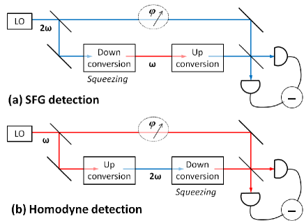
Figure 1: (Color online) (a) The proposed SFG scheme for measurement of squeezing: a narrowband pump local oscillator (LO) at frequency 2ω2𝜔2\omega is down-converted to generate squeezed light. To measure the obtained squeezing the light is first up-converted back to the pump frequency and the quadratures of the resulting SFG are measured by homodyning against the pump LO while varying its phase φ𝜑\varphi. This SFG scheme is a symmetric inversion of the standard homodyne scheme shown in (b), where a LO at ω𝜔\omega is first frequency doubled to 2ω2𝜔2\omega and then down-converted to 
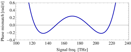
generate squeezing, which is measured by homodyning against the LO.
Refer to caption
Figure 2: Ultra-broad phase matching for SFG in a 1cm long PPKTP crystal with input near zero dispersion. $\!<\!0.25\pi$ phase mismatch is maintained over $\!\sim\!100THz$ input bandwidth for collinear SFG into 340THz (880nm).

We suggest a simple method to detect high-power two-mode squeezing, as produced by parametric oscillators above threshold SAT (1989); Villar et al. (2005); Pe er et al. (2006). The method, shown in Fig. 1, utilizes sum-frequency generation (SFG) as a detector of quantum correlation that is robust to detection inefficiency and accepts arbitrary frequency separation between the two modes. Previously, SFG was explored as an ultra-broadband two-photon detector in the low power regime of entangled bi-photons (squeezed vacuum), resolving simultaneously the tight time-difference and energy-sum correlation Dayan et al. (2005); Pe’er et al. (2005). In the proposed scheme, the degree of squeezing of the input is deduced from analysis of the quadrature noise of the SFG output.

The Robustness of SFG detection to inefficiency is motivated by the fact that as opposed to homodyne, detection efficiency of the (double-frequency) SFG photons is easily distinguishable from loss of squeezed (fundamental frequency) photons. Furthermore, SFG involves annihilation of photon in pairs, which for low input depletion (low SFG efficiency) preserves the quantum correlation within the squeezed input. The ability to detect two-mode squeezing of arbitrary separation is motivated by the fact that the SFG phase is equal to the phase-sum of the input modes. Consequently, homodyne detection of the SFG phase against the original pump measures the inter-mode phase correlation regardless of their separation. The detection bandwidth with SFG is therefore only limited by phase matching, which can be very broad for type-I phase matching Dayan et al. (2004, 2005); Peer et al. (2004), as shown in figure 2.

In what follows, we consider a fully quantum model of the SFG setup of Fig. 1(a) and derive in linear response approximation analytic expressions relating the input degree of squeezing to the measured spectral variance of the SFG output. We employ the positive-P representation Prep (1997); Gardiner (2004) - a general method for treatment of quantum correlations - to analyze SFG detection in realistic configurations, taking into account both loss and inefficiency. We start with a standard Hamiltonian LTS (2002); OptActa28 (1981)

$$\hat{H}=\hat{H}_{S}+\hat{H}_{R}+\hat{V},$$ (1)

where, setting $\hbar=1$,

$$\begin{split}\hat{H}_{S}=&\sum_{\alpha=i,s,2}\omega_{\alpha}\hat{a}^{\dagger}_{\alpha}\hat{a}_{\alpha}-i\frac{\chi}{2}\left(\hat{a}^{\dagger}_{2}\hat{a}_{i}\hat{a}_{s}-\!\emph{h.c}\right)\cr\quad&+i\left({\cal E}{\rm e}^{-i\omega_{s}t}\hat{a}_{s}^{{\dagger}}+{\cal E}^{*}{\rm e}^{-i\omega_{i}t}\hat{a}_{i}^{{\dagger}}-\!\emph{h.c}\right),\end{split}$$ (2)

is the SFG intra-cavity Hamiltonian including the non-linear interaction between the photon operators $\hat{a}_{s},\hat{a}_{i}$ and $\hat{a}_{2}$ of the signal, idler and SFG modes respectively, whose frequencies obey energy conservation $\omega_{i}+\omega_{s}=\omega_{2}$. The signal and the idler are driven by classical pumps ${\cal E}=|{\cal E}|{\rm e}^{-i\phi}$ and ${\cal E}^{*}$ that are complex conjugates to reflect the classical correlation between them Abram et al. (1986); Dayan et al. (2004); Harris (2007). $\hat{H}_{R}\!=\!\sum_{k}\!\omega_{k}\!\hat{b}^{\dagger}_{k}\!\hat{b}_{k}$, is the Hamiltonian of the loss reservoir of extra-cavity modes. In rotating wave approximation, the cavity modes are coupled to the loss reservoir by Scully (1997)

$$\hat{V}=\sum_{\alpha=i,s}\sum_{k}g_{\alpha k}\left(\hat{b}^{\dagger}_{k}\hat{a}_{\alpha}+\!\emph{h.c}\right).$$ (3)

To describe driving of a cavity by a quantum input, it is standard procedure to separate the average classical field from the quantum fluctuations. Just as driving by a coherent-state $|{\cal E}\rangle$ can be described as coupling to a classical pump ${\cal E}$ accompanied by a vacuum $|0\rangle$ input from the reservoir, we describe driving by a squeezed coherent state $|{\cal E},R{\rm e}^{i\theta}\rangle$ ($R$ - the degree of squeezing) as a classical pump ${\cal E}$ accompanied by a squeezed vacuum $|0,R{\rm e}^{i\theta}\rangle$ input from the reservoir.

It is useful to transform the mode basis from the signal and idler modes to collective modes, defined as

$$\hat{a}_{\pm}=\frac{1}{\sqrt{2}}\left(\hat{a}_{s}{\rm e}^{i\phi}\pm\hat{a}_{i}{\rm e}^{-i\phi}\right).$$ (4)

From classical analogy, the collective $\pm$ modes correspond to a carrier at the center frequency $\omega_{1}\!=\!(\omega_{i}\!+\!\omega_{s})/2\!=\!\omega_{2}/2$ modulated by a cosine or sine envelope at frequency $(\omega_{s}\!-\!\omega_{i})/2$. Just like $a_{s},a_{i}$, the collective operators commute $\left[a_{+},a_{-}\right]\!=\!\left[a_{+}^{{\dagger}},a_{-}^{{\dagger}}\right]\!=\!\left[a_{+},a_{-}^{{\dagger}}\right]\!=\!0$ and should not be confused with quadrature operators. Assuming $\langle\hat{b}_{k}\rangle=\langle\hat{b}^{\dagger}_{k}\rangle=0$, and using squeezed vacuum correlation functions Gardiner (2004)

$$\begin{split}&\langle\hat{b}^{\dagger}_{k}\hat{b}_{k^{\prime}}\rangle=N\delta\left(k,k^{\prime}\right),\ \ \langle\hat{b}_{k}\hat{b}^{\dagger}_{k^{\prime}}\rangle=(N+1)\delta\left(k-k^{\prime}\right),\\ &\langle\hat{b}^{\dagger}_{k}\hat{b}^{\dagger}_{k^{\prime}}\rangle=\langle\hat{b}_{k}\hat{b}_{k^{\prime}}\rangle^{*}=-M\delta\left(\omega_{k},\omega_{2}-\omega_{k^{\prime}}\right),\end{split}$$ (5)

we can substitute $\hat{a}_{s,i}\!=\!\left(\hat{a}_{+}\pm\hat{a}_{-}\right){\rm e}^{\pm i\phi}/{\sqrt{2}}$ (Eq. (4)) into the Hamiltonian and apply general methods to construct a reduced master equation in the Markovian limit Scully (1997):

$$\begin{split}\frac{d\hat{\rho}}{dt}=&-i\left[\hat{H}_{int},\hat{\rho}\right]+\gamma_{2}\left(2\hat{a}_{2}\hat{\rho}\hat{a}_{2}^{\dagger}-\hat{a}_{2}^{\dagger}\hat{a}_{2}\hat{\rho}-\hat{\rho}\hat{a}_{2}^{\dagger}\hat{a}_{2}\right)\\ &-{\cal N}\left[\hat{a}_{+}\right]+{\cal M}\left[\hat{a}_{+}\right]-{\cal N}\left[\hat{a}_{-}\right]-{\cal M}\left[\hat{a}_{-}\right],\end{split}$$ (6)

where

$$\hat{H}_{int}\!=\!i\sqrt{2}|{\cal E}|\left(\hat{a}^{\dagger}_{+}\!-\!\hat{a}_{+}\right)\!-\!i\frac{\chi}{4}\left(\hat{a}_{2}^{\dagger}\hat{a}_{+}^{2}\!+\!\hat{a}_{2}^{\dagger}\hat{a}_{-}^{2}\!-\!\emph{h.c}\right)$$ (7)

is the system Hamiltonian $\hat{H}_{S}$ in the interaction picture representation, and the functions $\cal N,\cal M$ are defined as

$$\begin{split}{\cal N}\left[\hat{A}\right]\!\equiv\!\gamma_{1}(N+1)\left[\hat{A}^{\dagger}\hat{A}\hat{\rho}-2\hat{A}\hat{\rho}\hat{A}^{\dagger}+\hat{\rho}\hat{A}^{\dagger}\hat{A}\right]\cr\quad+\gamma_{1}N\left[\hat{A}\hat{A}^{\dagger}\hat{\rho}-2\hat{A}^{\dagger}\hat{\rho}\hat{A}+\hat{\rho}\hat{A}\hat{A}^{\dagger}\right],\cr{\cal M}\left[\hat{A}\right]\!\equiv\!\gamma_{1}M\left[\hat{A}^{2}\hat{\rho}-2\hat{A}\hat{\rho}\hat{A}+\hat{\rho}\hat{A}^{2}\right]+\!\emph{h.c},\end{split}$$ (8)

and $\gamma_{1},\gamma_{2}$ are the decay rates of the signal $\pm$ idler and the SFG modes respectively. The quantities $M$ and $N$, appearing in Eqs. (8), characterize the input squeezing and, in principle, can be varied independently GardinerCollett (1985). For the ideal squeezed input, however, $M\!=\!\sinh(2R){\rm e}^{-i\theta}/2$, $N\!=\!\sinh^{2}(R)$, and hence, $|M|\!=\!\sqrt{N(N+1)}\!\approx\!N+1/2$. While arbitrary $\theta$ can be treated, we confine our analysis to real $M$ $(\theta\!=\!0,\pi)$ for brevity of expressions.

It is readily seen from Eq. (7) that with the definition of collective modes (Eq. (4)) only the cosine envelope $\hat{a}_{+}$ is driven directly, while the sine envelope $\hat{a}_{-}$ is neither externally excited nor directly coupled to $\hat{a}_{+}$. The only mechanism to populate $\hat{a}_{-}$ is by spontaneous down conversion from the created SFG field, which is negligible if the SFG efficiency is low. The physical picture of the two-mode SFG reduces therefore to that of a degenerate squeezing, apart from the modulation of the $\omega_{1}$ frequency carrier by a cosine envelope. Discarding the terms involving $\hat{a}_{-},\hat{a}_{-}^{\dagger}$ and setting $\hat{a}_{+}\!=\!\hat{a}_{1}$, Eqs. (6,7) take the form

$$\begin{split}&\frac{d\hat{\rho}}{dt}\!=\!i\left[\hat{\rho},\hat{H}_{int}\right]\!-\!\sum_{j=1,2}\!\gamma_{j}\!\left(\hat{a}_{j}^{\dagger}\hat{a}_{j}\hat{\rho}\!+\!\hat{\rho}\hat{a}_{j}^{\dagger}\hat{a}_{j}\!-\!2\hat{a}_{j}\hat{\rho}\hat{a}_{j}^{\dagger}\right)\cr&\!-\!2\gamma_{1}N\left[\hat{a}_{1}^{\dagger},\left[\hat{a}_{1},\hat{\rho}\right]\right]\!+\!\gamma_{1}M\left(\hat{a}_{1}^{2}\hat{\rho}\!+\!\hat{\rho}\hat{a}_{1}^{2}\!-\!2\hat{a}_{1}\hat{\rho}\hat{a}_{1}\!+\!\emph{h.c}\right)\!,\cr\quad&\hat{H}_{int}=i\sqrt{2}|{\cal E}|\left(\hat{a}^{\dagger}_{1}-\hat{a}_{1}\right)-i\frac{\chi}{4}\left(\hat{a}_{2}^{\dagger}\hat{a}_{1}^{2}-\emph{h.c}\right).\end{split}$$ (9)

With re-scaling ${\cal E}^{\prime}\!=\!\sqrt{2}|{\cal E}|,\!\ \!\chi^{\prime}\!=\!{\chi}/{2}$, Eqs. (9) coincide with the master equations obtained for degenerate SFG, leading to a unified formulation of two-mode SFG for any mode pair, regardless of the frequency separation.

For a fully quantum treatment we apply now the positive P-representation method Prep (1997); Gardiner (2004) to Eq. (9), which yields Itô stochastic differential equations (SDE’s)

$$\begin{split}&\left[\begin{array}[]{c}\frac{\partial}{\partial t}\alpha_{1}\\ \frac{\partial}{\partial t}\alpha_{1}^{+}\end{array}\right]=\left[\begin{array}[]{c}-\gamma_{1}\alpha_{1}+\chi^{\prime}\alpha_{1}^{+}\alpha_{2}+{\cal E}^{\prime}\\ -\gamma_{1}\alpha_{1}^{+}+\chi^{\prime}\alpha_{1}\alpha_{2}^{+}+{\cal E}^{\prime}\end{array}\right]+\\ &\ \ \ \ \ \ \ +\left[\begin{array}[]{cc}\chi^{\prime}\alpha_{2}+2\gamma_{1}M&2\gamma_{1}N\\ 2\gamma_{1}N&\chi^{\prime}\alpha_{2}^{+}+2\gamma_{1}M\end{array}\right]^{\frac{1}{2}}\left[\begin{array}[]{c}w_{1}(t)\\ w_{2}(t)\end{array}\right]\\ &\left[\begin{array}[]{c}\frac{\partial}{\partial t}\alpha_{2}\\ \frac{\partial}{\partial t}\alpha_{2}^{+}\end{array}\right]=\left[\begin{array}[]{c}-\gamma_{2}\alpha_{2}-\frac{\chi^{\prime}}{2}\alpha_{1}^{2}\\ -\gamma_{1}\alpha_{2}^{+}-\frac{\chi^{\prime}}{2}\alpha_{1}^{+^{2}}\end{array}\right],\end{split}$$ (10)

where $\alpha_{1},\alpha_{1}^{+},\alpha_{2},\alpha_{2}^{+}$ are independent c-number stochastic variables associated with the field operators, and $w_{1}(t),w_{2}(t)$ are real Gaussian noises, obeying

$$\langle w_{k}(t)\rangle=0,~{}~{}~{}\langle w_{j}(t)w_{k}(t^{\prime})\rangle=\delta_{jk}\delta(t-t^{\prime}).$$ (11)

Defining the normally ordered intra-cavity quadratures

$$q_{j}=\alpha_{j}+\alpha_{j}^{+},~{}~{}~{}p_{j}=-i(\alpha_{j}-\alpha_{j}^{+}),$$ (12)

and re-scaling with respect to $\gamma_{1}$ ($\tau\!\equiv\!\gamma_{1}t,\gamma_{r}\!\equiv\!\gamma_{2}/\gamma_{1},\mu\!\equiv\!{\cal E}^{\prime}/\gamma_{1}$), we obtain from SDE’s (10)

$$\begin{split}&\left[\begin{array}[]{c}\frac{\partial}{\partial\tau}q_{1}\\ \frac{\partial}{\partial\tau}p_{1}\end{array}\right]=\left[\begin{array}[]{c}2\mu-q_{1}+{\rm g}\sqrt{\frac{\gamma_{r}}{2}}(q_{1}q_{2}+p_{1}p_{2})\\ -p_{1}+{\rm g}\sqrt{\frac{\gamma_{r}}{2}}(q_{1}p_{2}-q_{2}p_{1})\end{array}\right]+\left[\begin{array}[]{cc}1&1\\ -i&i\end{array}\right]\cdot\\ &\cdot\left[\begin{array}[]{cc}{\rm g}\sqrt{\frac{\gamma_{r}}{2}}\left(q_{2}\!+\!ip_{2}\right)\!+\!2M&2N\\ 2N&{\rm g}\sqrt{\frac{\gamma_{r}}{2}}\left(q_{2}\!-\!ip_{2}\right)\!+\!2M\end{array}\right]^{\frac{1}{2}}\!\left[\begin{array}[]{c}w_{1}(\tau)\\ w_{2}(\tau)\end{array}\right],\\ &\left[\begin{array}[]{c}\frac{\partial}{\partial\tau}q_{2}\\ \frac{\partial}{\partial\tau}p_{2}\end{array}\right]=\left[\begin{array}[]{c}-\gamma_{r}q_{2}-{\rm g}\sqrt{\frac{\gamma_{r}}{8}}(q_{1}^{2}-p_{1}^{2})\\ -\gamma_{r}p_{2}-{\rm g}\sqrt{\frac{\gamma_{r}}{2}}q_{1}p_{1}\end{array}\right],\end{split}$$ (13)

where ${\rm g}\equiv{\chi^{\prime}}/{\sqrt{2\gamma_{1}\gamma_{2}}}$ characterizes the strength of the quantum fluctuations internal to the SFG cavity LTS (2002). For any classical amplitude ${\cal E}^{\prime}$ the validity of Eqs. (13) is guaranteed if the ratio of nonlinearity to damping ${\chi^{\prime}}/{\gamma_{j}}$ is small Prep (1997); LTS (2002). Note that Eqs. (13) contain two independent quantum noise contributions: one from the external noise induced by the coupling to the squeezed light, represented by $M$ and $N$; and the other - the internal noise proportional to the intra-cavity SFG field amplitude $\alpha_{2}=q_{2}+ip_{2}$, arising from the non-linear interaction. An important consequence is that for low SFG efficiency, the intra-cavity noise may be neglected compared to the squeezed input noise, which proves crucial for the SFG detection accuracy calculated below.

Eqs. (13) are complicated to be solved exactly. However, if the input noise is small compared to the classical terms (a reasonable assumption for an OPO well above threshold OPOAT (1990)), linearization methods can be justified to obtain approximate results OptActa28 (1981); Strogatz (2001). Within the zero-order approximation, corresponding to the classical dynamics, we discard the noise terms and obtain

$$\begin{split}&\frac{d}{d\tau}q^{(0)}_{1}\!=-q^{(0)}_{1}\!+2\mu+\!{\rm g}\sqrt{\frac{\gamma_{r}}{2}}(q^{(0)}_{1}q^{(0)}_{2}\!+\!p^{(0)}_{1}p^{(0)}_{2}),\\ &\frac{d}{d\tau}p^{(0)}_{1}\!=\!-p^{(0)}_{1}\!+\!{\rm g}\sqrt{\frac{\gamma_{r}}{2}}(q^{(0)}_{1}p^{(0)}_{2}\!-\!q^{(0)}_{2}p^{(0)}_{1}),\\ &\frac{d}{d\tau}q^{(0)}_{2}=-\gamma_{r}q^{(0)}_{2}-{\rm g}\sqrt{\frac{\gamma_{r}}{8}}(q^{(0)}_{1}q^{(0)}_{1}-p^{(0)}_{1}p^{(0)}_{1}),\\ &\frac{d}{d\tau}p^{(0)}_{2}=-\gamma_{r}p^{(0)}_{2}-{\rm g}\sqrt{\frac{\gamma_{r}}{2}}q^{(0)}_{1}p^{(0)}_{1}.\end{split}$$ (14)

The steady-state solution of Eqs. (14) (setting all time derivatives to zero) yields

$$\begin{split}&p^{(0)}_{1}=p^{(0)}_{2}=0,~{}~{}~{}~{}q^{(0)}_{2}=-\frac{{\rm g}}{\sqrt{8\gamma_{r}}}q^{(0)}_{1}q^{(0)}_{1},\\ &q^{(0)}_{1}=\frac{-2\sqrt[3]{6}+\sqrt[3]{4\left(9{\rm g}\mu+\sqrt{12+81{\rm g}^{2}\mu^{2}}\right)^{2}}}{\sqrt[3]{9}{\rm g}\sqrt[3]{\left(9{\rm g}\mu+\sqrt{12+81{\rm g}^{2}\mu^{2}}\right)}}\xrightarrow[g\rightarrow 0]{}2\mu.\end{split}$$ (15)

To investigate the temporal behavior of the system within the first order approximation we now substitute the zero-order solution Eqs. (15) into the noisy terms of Eqs. (13) and linearize the equations with respect to the deterministic part OptActa28 (1981); Strogatz (2001). This leads to

$$\begin{split}&\frac{d}{d\tau}\delta q_{1}\!=\!-\!\left(1\!+\!\frac{\nu^{2}}{4}\right)\!\delta q_{1}\!+\sqrt{\frac{\gamma_{r}}{2}}\nu\delta q_{2}\!+\!2\sqrt{M\!+\!N\!-\!\frac{\nu^{2}}{8}}~{}w_{+},\\ &\frac{d}{d\tau}\delta p_{1}\!=\!-\!\left(1\!-\!\frac{\nu^{2}}{4}\right)\!\delta p_{1}\!+\!\sqrt{\frac{\gamma_{r}}{2}}\nu\delta p_{2}\!-\!2i\sqrt{M\!-\!N\!-\!\frac{\nu^{2}}{8}}~{}w_{-},\\ &\frac{d}{d\tau}\delta q_{2}\!=\!-\!\sqrt{\frac{\gamma_{r}}{2}}\nu\delta q_{1}\!-\!\gamma_{r}\delta q_{2},~{}~{}~{}\frac{d}{d\tau}\delta p_{2}\!=\!-\!\sqrt{\frac{\gamma_{r}}{2}}\nu\delta p_{1}\!-\!\gamma_{r}\delta p_{2},\end{split}$$ (16)

where $\nu\!=\!{\rm g}q_{1}^{(0)}$ is a measure of the SFG efficiency $\eta_{SFG}\!=\!\nu^{2}/8$ and $w_{\pm}\!=\!\left[w_{1}\!\pm\!w_{2}\right]/\sqrt{2}$ represent white noises.

Eqs. (16) can be solved in Fourier space to obtain the desired SFG quadratures

$$\begin{split}&\delta\tilde{q}_{2}(\Omega)=-\frac{\nu\sqrt{2\gamma_{r}}\sqrt{M+N-\frac{\nu^{2}}{8}}~{}\tilde{w}_{+}(\Omega)}{\gamma_{r}\left(1+\frac{3\nu^{2}}{4}\right)+i\left(1+\gamma_{r}+\frac{\nu^{2}}{4}\right)\Omega-\Omega^{2}},\\ &\delta\tilde{p}_{2}(\Omega)=i\frac{\nu\sqrt{2\gamma_{r}}\sqrt{M-N-\frac{\nu^{2}}{8}}~{}\tilde{w}_{-}(\Omega)}{\gamma_{r}\left(1+\frac{\nu^{2}}{4}\right)+i\left(1+\gamma_{r}-\frac{\nu^{2}}{4}\right)\Omega-\Omega^{2}}.\end{split}$$ (17)

Using Eqs. (17) and the correlation properties of white noise $\langle\tilde{w}_{j}(\Omega_{1})\tilde{w}_{k}(\Omega_{2})\rangle=\delta_{jk}\delta(\Omega_{1}+\Omega_{2})$ we find

$$\begin{split}\langle&\delta\tilde{q}_{2}(\Omega_{1})\delta\tilde{q}_{2}(\Omega_{2})\rangle=\\ &=\frac{2\gamma_{r}\nu^{2}\left(N\!+\!M-\frac{\nu^{2}}{8}\right)\delta(\Omega_{1}\!+\!\Omega_{2})}{\gamma_{r}^{2}\left(1\!+\!\frac{3\nu^{2}}{4}\right)^{2}\!+\!\gamma_{r}^{2}\Omega^{2}\left(1\!-\!\frac{\nu^{2}}{\gamma_{r}}\right)\!+\!\Omega^{2}\left(1\!+\!\frac{\nu^{2}}{4}\right)^{2}\!+\!\Omega^{4}},\\ &\langle\delta\tilde{p}_{2}(\Omega_{1})\delta\tilde{p}_{2}(\Omega_{2})\rangle=\\ &=\frac{2\gamma_{r}\nu^{2}\left(N\!-\!M\!+\!\frac{\nu^{2}}{8}\right)\delta(\Omega_{1}\!+\!\Omega_{2})}{\gamma_{r}^{2}\left(1\!+\!\frac{\nu^{2}}{4}\right)^{2}\!+\!\gamma_{r}^{2}\Omega^{2}\left(1\!-\!\frac{\nu^{2}}{\gamma_{r}}\right)\!+\!\Omega^{2}\left(1\!-\!\frac{\nu^{2}}{4}\right)^{2}\!+\!\Omega^{4}},\end{split}$$ (18)

which express the intra-cavity SFG spectral variances (normally ordered) in terms of the squeezing parameters $N\!+\!M$ and $N\!-\!M$. When $N\!-\!M$ dominates over the internal noise ($N\!-\!M\!\gg\!{\nu^{2}}/{8}$), the SFG quadratures fluctuations directly provide the degree of input squeezing.

Since measurements are performed on the fields outside the cavity, we now transform the intra-cavity spectral variances in Eqs. (18) to extra-cavity spectral variances using the input-output relation $\hat{\Phi}_{j}^{out}\!=\!\sqrt{2\gamma_{j}^{out}}\hat{a}_{j}\!-\!\hat{\Phi}_{j}^{in}$ GardinerCollett (1985), where $\hat{\Phi}_{j}^{out},\hat{\Phi}_{j}^{in}$ are the outgoing and incoming photon operators external to the cavity and $\hat{a}_{j}$ is the intra-cavity operator whose dynamics we have studied so far. For simplicity, we assume $\gamma_{j}^{out}\!=\!\gamma_{j}$, indicating a lossless cavity where damping is only due to output coupling. Defining general quadratures $\hat{X}_{j}^{\theta}\!=\!\left({\rm e}^{-i\theta}\hat{\Phi}^{out}_{j}\!+\!{\rm e}^{i\theta}\hat{\Phi}^{out^{\dagger}}_{j}\right)$ the output spectral variance $V^{\theta}_{j}(\Omega)$ can be written as LTS (2002)

$$V_{j}^{\theta}(\omega)\delta(\omega+\omega^{\prime})=1+\langle\Delta X_{j}^{\theta}(\omega)\Delta X_{j}^{\theta}(\omega)\rangle_{\textsc{p}},$$ (19)

where the subscript ${\rm P}$ stands for the normal ordering, $\Delta X_{j}^{\theta}\equiv X_{j}^{\theta}-\langle X_{j}^{\theta}\rangle$ and the frequency argument denotes a Fourier transform $\tilde{X}_{j}^{\theta}(\omega)=\int\frac{dt}{\sqrt{2\pi}}{\rm e}^{i\omega t}X_{j}^{\theta}(t)$.

It is essential that the input field $\Phi_{1}^{in}$, which is associated with the input noise term in Eqs. (10) for the intra-cavity fields, is properly included. However, for the SFG mode 2, which is not explicitly driven by any noise ($\Phi_{2}^{in}=0$), $V^{\theta}_{2}(\omega)$ takes the form LTS (2002); GardinerCollett (1985)

$$V^{\theta}_{2}(\omega)\delta(\omega+\omega^{\prime})=1+2\gamma_{2}\langle\Delta\tilde{x}^{\theta}_{2}(\omega)\Delta\tilde{x}^{\theta}_{2}(\omega^{\prime})\rangle_{\textsc{p}},$$ (20)

where $\tilde{x}^{\theta}_{j}$ is the generalized intra-cavity quadrature. Remembering the re-scaling of time by $\gamma_{1}$, on substituting Eqs. (18) into Eq. (20), we obtain the desired relations between the measured extra-cavity SFG quadratures and the squeezing parameters of the input field:

$$\begin{split}&V^{0}_{2}(\Omega)=1+\\ &+\frac{4\gamma_{r}^{2}\nu^{2}\left(N\!+\!M-\frac{\nu^{2}}{8}\right)}{\gamma_{r}^{2}\left(1\!+\!\frac{3\nu^{2}}{4}\right)^{2}\!+\!\gamma_{r}^{2}\Omega^{2}\left(1\!-\!\frac{\nu^{2}}{\gamma_{r}}\right)\!+\!\Omega^{2}\left(1\!+\!\frac{\nu^{2}}{4}\right)^{2}\!+\!\Omega^{4}},\\ &V^{\frac{\pi}{2}}_{2}(\Omega)=1+\\ &+\frac{4\gamma_{r}^{2}\nu^{2}\left(N\!-\!M+\frac{\nu^{2}}{8}\right)}{\gamma_{r}^{2}\left(1\!+\!\frac{\nu^{2}}{4}\right)^{2}\!+\!\gamma_{r}^{2}\Omega^{2}\left(1\!-\!\frac{\nu^{2}}{\gamma_{r}}\right)\!+\!\Omega^{2}\left(1\!-\!\frac{\nu^{2}}{4}\right)^{2}\!+\!\Omega^{4}}.\end{split}$$ (21)

By construction within the positive-P representation, Eqs. (21) represent a realistic measurement of the extra-cavity SFG quadratures with either partially or ideally squeezed input. The only assumptions are that the SFG cavity is lossless for the input squeezed light (such loss would hinder the squeezing like any other loss) and that the photo-detector efficiency is included in the SFG efficiency ηSFG=ν2/8subscript𝜂𝑆𝐹𝐺superscript𝜈28\eta_{SFG}\!=\!\nu^{2}/8. 
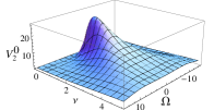
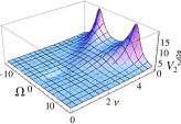
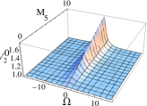
Figure 3 illustrates the results of Eqs. (21) for an ideally squeezed input M=N(N+1)𝑀𝑁𝑁1M=\sqrt{N(N+1)} at realistic parameters. As evident, the measured SFG quadratures are either non-squeezed (in Q𝑄Q quadrature) or undergo insignificant squeezing (in P𝑃P quadrature). Moreover, for non-ideal squeezed input, where N>|M|𝑁𝑀N>|M|, fluctuations of both SFG quadratures are always above the SQL, which indicates the robustness of the proposed detection to loss of SFG photons, as sub-SQL fluctuations need not be detected. We also note that for a non-squeezed input (M=N=0𝑀𝑁0M\!=\!N\!=\!0) Eqs. (21) yield slight squeezing of the SFG output, a known result in SFG cavities sSFG (2???). This squeezing is negligible compared to the external input noise for low SFG efficiency.

Refer to caption Refer to caption

(a)γr=M=10𝑎subscript𝛾𝑟𝑀10(a)\gamma_{r}=M=10
(b)γr=M=10𝑏subscript𝛾𝑟𝑀10(b)\gamma_{r}=M=10

Refer to caption
Refer to caption

(c)γr=10,ν=0.1formulae-sequence𝑐subscript𝛾𝑟10𝜈0.1(c)\gamma_{r}=10,\nu=0.1
(d)γr=10,ν=0.1formulae-sequence𝑑subscript𝛾𝑟10𝜈0.1(d)\gamma_{r}=10,\nu=0.1
Figure 3: The plot of $V^{0}_{2}(\Omega)$ Eq. (21) [(a) and (c)] and of $V^{\frac{\pi}{2}}_{2}(\Omega)$ [(b) and (d)] for ideally squeezed input $M=\sqrt{N(N+1)}$ as functions of the scaled frequency $\Omega$, the squeezing parameter $M$, with $\nu={\rm g}q_{1}^{(0)}$, ${\rm g}={\chi^{\prime}}/{\sqrt{2\gamma_{1}\gamma_{2}}}$ and $q_{1}^{(0)}$ given by Eq. (15).

Finally, we can use Eqs. 21 to estimate the sensitivity limit of our scheme and the optimal efficiency $\eta_{SFG}\!=\!\nu^{2}/8$. Assuming a fast SFG cavity ($\gamma_{r}^{2}\!=\!\left(\gamma_{2}/\gamma_{1}\right)^{2}\!\gg\!\Omega^{2}$), Eqs. (21) can be expanded to 4th order in $\nu$, yielding

$$\begin{split}&V^{0}_{2}(\Omega)\approx 1\!+\!\frac{4\nu^{2}}{1\!+\!\Omega^{2}}\left[(N\!+\!M)\!-\!\frac{\nu^{2}}{8}\left(1\!+\!\frac{3}{4}\frac{N\!+\!M}{1\!+\Omega^{2}}\right)\right],\\ &V^{\frac{\pi}{2}}_{2}(\Omega)\approx 1\!+\!\frac{4\nu^{2}}{1\!+\!\Omega^{2}}\left[(N\!-\!M)\!+\!\frac{\nu^{2}}{8}\left(1\!-\!\frac{1}{4}\frac{N\!-\!M}{1\!+\Omega^{2}}\right)\right].\end{split}$$ (22)

Measurement of the squeezing parameters $N-M$, $N+M$ may be obscured either by vacuum noise (SQL) for low SFG efficiency (the first ${}^{\prime}1^{\prime}$ term) or by the internal SFG noise for high efficiency due to input depletion (the last term). The minimum detectable $(N-M)$ is obtained when all contributions are similar $4\nu^{2}(N-M)\!=\!1\ and\ (N-M)\!=\!\nu^{2}/8$, indicating that optimal detection occurs for $\nu^{2}\!=\!\sqrt{2}$ or $\eta_{SFG}\!\approx\!0.18$, allowing detection down to $(N-M)_{min}\!\approx\!0.18$, very close to the ideal value $(N-M)_{ideal}\!\geq\!-\!1/2$. We expect therefore that this new method will find applications in high precision metrology.

This research was partially supported by the Marie Curie IRG program of the European Union.

References

  • Caves (1981) C. M. Caves, Phys. Rev. D 23, 1693 (1981).
  • Holland and Burnett (1993) M. J. Holland and K. Burnett, Phys. Rev. Lett. 71, 1355 (1993); T. Kim et al, Phys. Rev. A. 57, 4004 (1998).
  • Goda et al. (2008) K. Goda et al, Nature Physics 4, 472 (2008).
  • Polzik et al. (1992) E. S. Polzik, J. Carri and H. J. Kimble, Appl. Phys. B 55, 279 (1992).
  • Oblak et al. (2005) D. Oblak et al, Phys. Rev. A 71, 043807 (2005).
  • Abram et al. (1986) I. Abram, R. K. Raj, J. L. Oudar, and G. Dolique, Phys. Rev. Lett. 57, 2516 (1986).
  • Dayan et al. (2004) B. Dayan, A. Pe’er, A. A. Friesem, and Y. Silberberg, Phys. Rev. Lett. 93, 023005 (2004).
  • Peer et al. (2004) A. Pe’er, B. Dayan, Y. Silberberg, and A. A. Friesem, J. Lightwave Technol. 22, 1463 (2004).
  • Harris (2007) S. E. Harris, Phys. Rev. Lett. 98, 063602 (2007).
  • Villar et al. (2005) A. S. Villar et al, Phys. Rev. Lett. 95, 243603 (2005).
  • Takeno et al. (2007) Y. Takeno, M. Yukawa, H. Yonezawa and A. Furusawa, Opt. Express 15, 4321 (2007).
  • Vahlbruch et al. (2008) H. Vahlbruch et al, Phys. Rev. Lett. 100, 033602 (2008).
  • Pe er et al. (2006) A. Pe’er, Y. Silberberg, B. Dayan and A. A. Friesem, Phys. Rev. A 74, 053805 (2006).
  • SAT (1989) M. D. Reid and P. D. Drummond, Phys. Rev. A 40, 4493 (1989).
  • Dayan et al. (2005) B. Dayan, A. Pe’er, A. A. Friesem and Y. Silberberg, Phys. Rev. Lett. 94, 043602 (2005).
  • Pe’er et al. (2005) A. Pe’er, B. Dayan, A. A. Friesem and Y. Silberberg, Phys. Rev. Lett. 94, 073601 (2005).
  • Scully (1997) M. O. Scully, M. S. Zubairy “Quantum Optics”, Cambridge University Press (1997).
  • LTS (2002) S. Chaturvedi, K. Dechoum and P. D. Drummond, Phys. Rev. A 65, 033805 (2002).
  • OptActa28 (1981) P. D. Drummond, K. J. McNeil and D. F. Walls Opt. Acta 28, 211 (1981);
  • GardinerCollett (1985) C. W. Gardiner and M. J. Collett, Phys. Rev. A 31, 3761 (1985);
  • Prep (1997) A. Gilchrist, C. W. Gardiner and P. D. Drummond, Phys. Rev. A 55, 3014 (1997).
  • Gardiner (2004) C. W. Gardiner “Handbook of Stoachastic Methods” Springer-Verlag, Berlin Heidelberg (2004).
  • OPOAT (1990) M. D. Reid and P. D. Drummond, Phys. Rev. Lett. 60, 2731 (1988).
  • Strogatz (2001) S. H. Strogatz “Nonlinear Dynamics and Chaos” Westview Press, Reading, Massachusetts (2001).
  • sSFG (2???) S. F.  Pereira, M.  Xiao, H. J.  Kimble and J. L. Hall Phys. Rev. A 38, 4931 (1988).