The spectral types of white dwarfs in Messier 4

Abstract

We present the spectra of 24 white dwarfs in the direction of the globular cluster Messier 4 obtained with the Keck/LRIS and Gemini/GMOS spectrographs. Determining the spectral types of the stars in this sample, we find 24 type DA and 0 type DB (i.e., atmospheres dominated by hydrogen and helium respectively). Assuming the ratio of DA/DB observed in the field with effective temperature between $15\,000$–$25\,000$ K, i.e., 4.2:1, holds for the cluster environment, the chance of finding no DBs in our sample due simply to statistical fluctuations is only $6\times 10^{-3}$. The spectral types of the $\sim 100$ white dwarfs previously identified in open clusters indicate that DB formation is strongly suppressed in that environment. Furthermore, all the $\sim 10$ white dwarfs previously identified in other globular clusters are exclusively type DA. In the context of these two facts, this finding suggests that DB formation is suppressed in the cluster environment in general. Though no satisfactory explanation for this phenomenon exists, we discuss several possibilities.

1. Introduction

Because of their intrinsically faint luminosities, white dwarfs are relatively hard to study spectroscopically. It is now generally accepted that the number of DA to non-DA white dwarfs is a function of temperature (see Bergeron et al., 1997, for example). Because a given white dwarf will be born with a high temperature, and subsequently cool through the entire range of observed white-dwarf temperatures, the implication of this observation is that white dwarfs can change their spectral type multiple times throughout their evolution. This means that, unlike main-sequence stars, white dwarfs that are physically similar can have very different spectra, or vice-versa. The dominant physical variable that controls the spectral type of a white dwarf during its evolution is the mass of the very-thin atmosphere layer.

Hansen and Liebert (2003) outline the presumed multiple evolutionary sequences of white dwarfs with “thick” and “thin” hydrogen envelopes, with envelope masses of $10^{-4}\,M_{\odot}$ and $\sim 10^{-10}$$M_{\odot}$ respectively. Stars with thick hydrogen layers have atmospheres rich in hydrogen throughout their evolution, and will always appear as DAs (exhibiting H i lines). White dwarfs with thin hydrogen layers have a much more complicated evolution, and may at varying times have atmospheres dominated by either hydrogen or helium. These white dwarfs may be born with DA or DO (exhibiting He ii lines) spectral types. As the stars cool, helium ions will recombine, and the DOs will transform into DBs (exhibiting He i lines).

At temperatures between $30\,000$–$150\,000$ K, DAs far outnumber DBs. In fact, from $30\,000$–$45\,000$ K there is the so-called “DB gap” Liebert et al. (1986). This temperature range was, until recently, completely devoid of DB stars. With DR4, the SDSS had accumulated $10^{4}$ white-dwarf spectra, and within this sample, approximately 10 DB white dwarfs were found in this temperature range (Eisenstein et al., 2006b). While this temperature range is no longer strictly a “gap”, it is still true that the DA/DB ratio is approximately 2.5 times greater at $30\,000$ K than it is at $20\,000$ K. This implies that an atmospheric transformation takes place in approximately 10% of DAs as they cool through this range (Eisenstein et al., 2006b).

Below $30\,000$ K, a helium convection zone is established. Convective velocities can become high enough to overshoot, and mix the helium layer with the hydrogen atmosphere, converting a type DA to a type DB. This occurs in $\sim 25$% of white dwarfs in this temperature range in the field (Hansen and Liebert, 2003).

For temperatures lower than $6\,000$ K, the situation becomes even more complicated and uncertain (Bergeron et al., 1997). At these low temperatures the variety of spectral types increases, but in the non-DA gap ($6\,000$–$5\,000$ K) non-DA white dwarfs have yet to be observed. As white dwarfs cool below $5\,000$ K, neither hydrogen nor helium lines are excited, and the resultant spectrum is almost featureless, leading to the DC spectral classification. Even more rare are white dwarfs showing metal lines. These are the DQs, for those showing carbon features, and the DZs, for other atomic species. Finally, DP and DH white dwarfs show evidence of having polarized and non-polarized magnetic fields respectively.

Prior to the year 2000, the spectra of cluster white dwarfs had been obtained in a piecemeal fashion—only one or two stars would be studied in each cluster, typically by different authors. The Canada-France-Hawaii Telescope (CFHT) Open Star Cluster Survey changed this. The idea behind this survey was to obtain high-quality, wide-field images of many open clusters. The rich clusters (i.e., those with well-populated white dwarf cooling sequences) could then be identified, and followed up spectroscopically. Previously, when spectral types were obtained for only several white dwarfs at a time, the absence of a particular spectral type was neither particularly surprising nor interesting.

Kalirai et al. (2005) reported 21 spectral identifications in NGC 2099. Assuming the same DA/DB ratio observed in the field for this temperature range ($15\,000$ K–$30\,000$ K) held for this cluster, it was expected that several DB white dwarfs would be found. Contrary to expectations, no DB white dwarfs were found. According to Kalirai et al. (2005), finding a DB/DA ratio of 0/21 would occur approximately 2% of the time simply due to statistical fluctuations. This finding prompted Kalirai et al. (2005) to examine all white dwarf spectral identifications in young open clusters. These cluster were all very young. In fact, NGC 2099 was the oldest of the sample. Because turn-off mass (and therefore white-dwarf mass) is inversely correlated with cluster age, all of the white dwarfs in this sample are very massive. Of all the 65 white dwarfs that had been spectroscopically identified in young open clusters at that point, all were of type DA. This had a vanishingly small chance of occurring due to a statistical fluctuation under the hypothesis that the same DA/DB ratio held as in the field.

An obvious explanation for this observation was not apparent. One early explanation was the re-accretion of residual intra-cluster gas in open clusters. However, this explanation appeared not to hold up on closer examination. The escape velocity in open clusters is typically very low ($v_{\rm esc}\sim 1\,km\,s^{-1}$), and gas ejected by stellar winds ($v_{\rm wind}\sim 10\,km\,s^{-1}$) would be expected to quickly escape. It was found that the accretion rate of intra-cluster gas in open clusters should be no greater than that of the ISM in the disk. Kalirai et al. (2005) postulated an explanation based on the mass of the white dwarfs. Because NGC 2099 is a young cluster, the young white dwarfs are high mass ($\sim 0.8$ $M_{\odot}$) compared to the average disk population ($\sim 0.6$ $M_{\odot}$). He convection is inhibited in high-mass white dwarfs, and therefore even white dwarfs with thin hydrogen atmospheres would remain type DA in this temperature range.

Globular clusters are the oldest Galactic stellar population, and should therefore create the lowest-mass white dwarfs ($\sim 0.5$ $M_{\odot}$). It is of interest to determine whether the same paucity of DB white dwarfs exists in globular clusters. Recent observations suggest that the same paucity is indeed there. In 2004, Moehler et al. (2004) obtained spectra of $5$ white dwarfs in NGC 6752 and another $4$ in NGC 6397, all of which were found to be type DA. Assuming that the DA/DB ratio is the same as in the field, the chance of finding no DB white dwarfs given the number observed in NGC 6752 and NGC 6397 is 0.35 and 0.43 respectively.

The current paper follows from an ultra-deep HST/WFPC2 study of the nearest globular cluster, Messier 4 (NGC 6121) by Richer et al. (2002). White dwarfs identified in this photometry were followed up with the Gemini/GMOS and Keck/LRIS spectrographs. The primary science goal of the spectrographic follow-up was the determination of the masses of the white dwarfs (see Kalirai et al. 2009). While spectroscopic masses were determined for only a subset of the observed white dwarfs due to signal-to-noise ratio constraints, the spectral types were determined for 24 of the 25 candidates with a high-probability of being a white dwarf. The determination of the spectral type of 24 white dwarfs more than doubles the number of existing identifications of white dwarfs in globular clusters. As in the earlier studies, we find a complete lack of DBs in our sample.

2. Photometric target selection

A critical, and in this case particularly challenging, component of any spectroscopic study, is the target selection. We used two sources of pre-imaging to select stars that lie on the white-dwarf cooling curve of Messier 4. White dwarf candidates were selected from the WFPC2 photometry published in Richer et al. (2004), and from Gemini/GMOS imaging. These targets were followed up with the two multi-slit spectrographs: Gemini/GMOS and Keck/LRIS.

Our most secure white dwarf targets come from the WFPC2 photometry. Stars in these fields have their cluster membership confirmed by their proper motions. However, there are two limitations with the WFPC2 imaging. First, both the GMOS and the LRIS fields-of-view are much larger than the WFPC2 field. In order to maximize the number of spectra, we must distribute the targets evenly over the spectroscopic fields, and therefore some of our spectroscopic targets fell outside the WFPC2  field of view. Second, the PSFs of ground-based instruments are obviously much broader than that of the WFPC2. Some of the white dwarfs that are easily resolved with WFPC2  are lost in the scattered light from bright stars in ground-based photometry in this crowded field.

2.1. GMOS target selection

In order to obtain stars over the entire GMOS field, GMOS pre-imaging was obtained. The stars selected from the GMOS photometry could only be selected in colour-magnitude space, and not proper-motion space, and therefore their cluster membership is less certain. LRIS, GMOS, and WFPC2 all have different fields of view, and some areas of the sky have been studied with all three instruments, while others have only been studied by one or two. The footprints for the various instruments are shown in Figure 1.

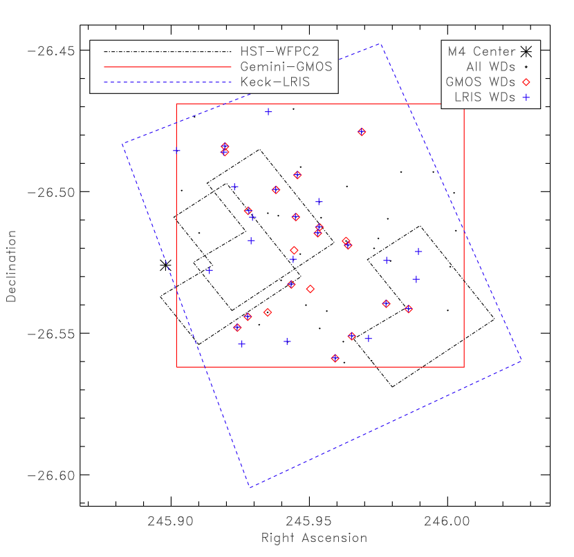
Figure 1.— The footprint of the HST/WFPC2, Gemini/GMOS, and Keck/LRIS instruments. The white dwarf candidates selected from the GMOS photometry (i.e., those stars with 21 $<$ F555W $<$ 25, and F555W-F814W $<$ 0.9.) are shown as dots. The objects targeted for GMOS spectroscopy are shown with diamonds. The objects targeted for LRIS spectroscopy are shown with pluses.

In order to effectively select white dwarf candidates over the entire GMOS field, pre-imaging was taken in both the g^′ and r^′ filters. The images were corrected for bias and flat fielding by the Gemini pipeline. The pre-processed images were then reduced with the standard DAOPHOT/Allstar reduction techniques (Stetson, 1987). This photometry was not used for anything other than the target selection, and hence was not rigorously calibrated. There are $10^{3}$ stars imaged both with WFPC2 and GMOS. In order to calibrate the GMOS photometry, a transformation between the GMOS and the calibrated WFPC2 photometry was determined. The transformation was of the form:

$$g-r = g^{\prime}-r^{\prime}-x_{0}$$

$$g = g^{\prime}-y_{0}$$

$$\text{F555W} = y_{0}+y_{1}\,g+y_{2}\,(g-r)+y_{3}\,(g-r)g$$

$$\text{F555W-F814W} = x_{0}+x_{1}\,g+x_{2}\,(g-r)+x_{3}\,(g-r)g$$

The coefficients were determined from minimizing $\chi^{2}$ using the downhill-simplex method Amoeba (Press et al., 1986), and were found to be: $x_{0}=19.0$, $x_{1}=1.72\times 10^{-3}$, $x_{2}=1.19\times 10^{-1}$, $x_{3}=1.12\times 10^{-2}$, $y_{0}=19$, $y_{1}=-2.02\times 10^{-1}$, $y_{2}=-4.59\times 10^{-3}$, and $y_{3}=-5.67\times 10^{-2}$.

The GMOS photometry was then transformed to the WFPC2 bands. The CMD constructed from the GMOS photometry is presented in Figure 2. A clear white dwarf cooling sequence can be seen beginning at F555W=22.5 and F555W-F814W=0.30.

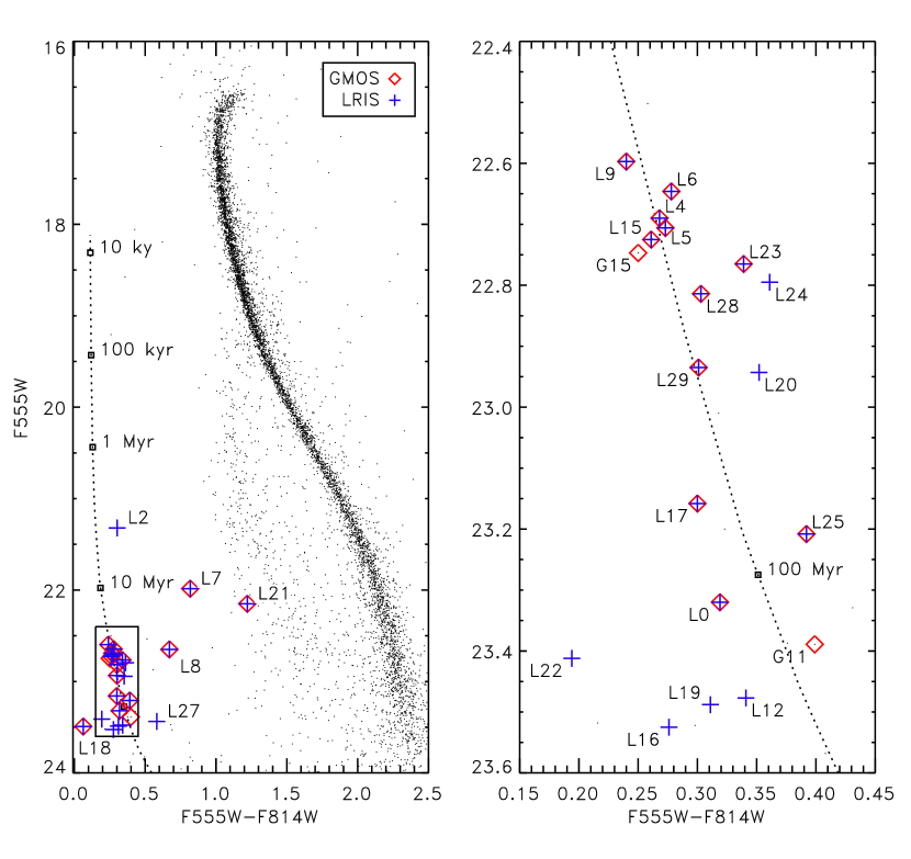
Figure 2.— The CMD constructed from the GMOS photometry. There is a clear white dwarf cooling sequence extending from $22.5<$F555W$<24$ with an approximate colour of F555W-F814W=0.3. The left panel shows the entire range, while the right panel shows only the white dwarf cooling sequence. A cooling sequence (assuming (m-M)_F814=12.49 and E(F555W-F814W)=0.06) of a 0.5 $M_{\odot}$ DA white dwarf is shown (Fontaine et al., 2001). The GMOS photometry in the white dwarf-region has been replaced by WFPC2 photometry where it exists.

Figure 1 shows the location of the white dwarf candidates selected from the GMOS photometry (points). Note the paucity of GMOS points in the inner WFPC2 fields. Though there are many white dwarfs here, the crowding is such that they become very difficult to detect with ground-based telescopes, such as Gemini. The GMOS points are those stars with magnitudes between F555W=22.5 and F555W=24.5 and colours less than F555W-F814W=0.9. All the relevant candidate selection measurements are tabulated in Table 1.

Table 1The measurements used for target selection and measured spectral type

LRIS #	GMOS #	RA	DEC	F555W-F814W	F555W	F555W-F814W	F555W
		(J2000)	(J2000)	(GMOS)		(WFPC2)
LRIS-0	GMOS-21	245.9579	-26.5589	0.319	23.320	—	—
LRIS-2	—	245.9406	-26.5531	0.302	21.321	—	—
LRIS-4	GMOS-20	245.9638	-26.5511	0.268	22.690	—	—
LRIS-5	GMOS-19	245.9224	-26.5480	0.273	22.706	—	—
LRIS-6	GMOS-18	245.9262	-26.5442	0.278	22.646	—	—
—	GMOS-15	245.9334	-26.5426	0.250	22.747	—	—
LRIS-7	GMOS-16	245.9844	-26.5414	0.818	21.985	—	—
LRIS-8	GMOS-13	245.9763	-26.5396	0.671	22.649	—	—
LRIS-9	GMOS-14	245.9419	-26.5328	0.258	22.502	0.240	22.597
LRIS-12	—	245.9427	-26.5241	0.216	23.518	0.341	23.477
—	GMOS-11	245.9617	-26.5174	0.399	23.389	—	—
LRIS-15	GMOS-10	245.9625	-26.5190	0.261	22.725	—	—
LRIS-16	—	245.9276	-26.5175	—	—	0.276	23.525
LRIS-17	GMOS-6	245.9515	-26.5147	0.323	23.200	0.300	23.158
LRIS-18	GMOS-8	245.9521	-26.5125	0.097	23.891	0.063	23.492
LRIS-19	—	245.9281	-26.5092	0.431	23.329	0.311	23.488
LRIS-20	GMOS-7	245.9436	-26.5090	0.318	23.010	0.352	22.943
LRIS-21	GMOS-9	245.9263	-26.5067	1.221	22.150	—	—
LRIS-22	—	245.9521	-26.5037	0.194	23.412	—	—
LRIS-23	GMOS-4	245.9364	-26.4994	0.513	22.536	0.339	22.765
LRIS-24	—	245.9216	-26.4984	0.262	22.724	0.361	22.795
LRIS-25	GMOS-3	245.9442	-26.4941	0.392	23.208	—	—
LRIS-27	—	245.9006	-26.4856	0.582	23.437	—	—
LRIS-28	GMOS-2	245.9179	-26.4840	0.303	22.814	—	—
LRIS-29	GMOS-1	245.9674	-26.4789	0.301	22.935	—	—

2.2. Keck target selection

We constructed a CMD from LRIS photometry, but it lacks a coherent white-dwarf-cooling sequence. Furthermore, by the time we were selecting targets for the LRIS mask, the GMOS spectroscopy had already been performed. We therefore had spectroscopic confirmation of many white dwarfs. The selection for LRIS was therefore performed with the same inputs as that for the GMOS photometry. The locations of the LRIS targets shown in the GMOS colour-magnitude space are shown in Figure 2, and their astrometry in Figure 1.

3. Spectral Reductions

3.1. GMOS Reductions

In total, we obtained approximately 14.5 and 9 hours of science exposure with GMOS in 2005A and 2006B respectively. Because of the queue system we were able to require all exposures to be obtained in sub-arcsecond seeing. The GMOS observations obtained are listed in Table 2. Our GMOSmask consisted of 21 objects. The slits were all 0$\farcs$8 wide and 5$\farcs$0 long. We used the B1200 grating, and binned by two pixels in the spectral direction resulting in a resolution of $R=1900$.

Table 2 Observing information

GMOS							LRIS
exposure	date	number of	seeing	airmass			exposure	date	number of	seeing	airmass
time (s)		exposures	(″)				time (s)		exposures	(″)
3600	06/06/2005	2	0.8	1.08–1.23			2700	04/21/2007	2	0.9	1.45–1.49
3600	06/07/2005	3	0.8	1.04–1.34			900	04/21/2007	1	1.0	1.64
1687	06/08/2005	1	0.8	1.45			2700	04/22/2007	3	1.0	1.45–1.52
3600	06/09/2005	5	0.8	1.02–1.45			1800	04/22/2007	1	1.0	1.56
3600	08/04/2005	2	0.8	1.13–1.33			1800	07/14/2007	2	1.0	1.45–1.63
3600	08/08/2005	1	0.8	1.03			2100	07/14/2007	1	1.2	1.52
620	08/08/2005	1	0.8	1.14			1800	07/15/2007	4	0.8	1.45–1.51
3600	08/09/2005	1	0.8	1.03–1.07			1800	04/12/2008	5	2.0	1.45–1.52
3600	08/19/2006	3	0.8	1.03–1.33
3600	08/20/2006	1	0.8	1.12
3600	08/21/2006	2	0.8	1.06–1.18
3600	09/15/2006	1	0.8	1.23
3600	09/16/2006	1	0.8	1.25
3600	09/20/2006	1	0.8	1.32

The raw data frames were downloaded from the Canadian Astronomy Data Center (CADC) in multi-extension FITS (MEF) format. We reduced the data using the Gemini iraf Package, version 1.4. GMOS is composed of three separate chips. The dispersion axis is perpendicular to the long axis of the chips, and therefore the dispersed spectra will cross the gaps between the chips, leaving gaps in the spectral coverage. The precise spectral coverage for a given star depends on its position in the detector, and is therefore slightly different for each star. Because the spectral range is different for each star, we are unable to choose a central wavelength such that no star will have a Balmer line that falls on a chip gap. To avoid a Balmer line falling on a gap and rendering the spectrum useless, we obtain the spectrum at two different grating offsets. This is equivalent to dithering a camera when obtaining imaging. The central wavelength was shifted from the default value of 4620 ${\rm\AA}$ to 4720 ${\rm\AA}$ for half of the exposures. These two sets of spectra are handled separately until the wavelength calibration is determined.

The GMOS data were reduced using the iraf/Gemini package. For the initial stages of the reductions, the standard steps, i.e., gprepare (updates FITS header information, and associates image with mask definition file), gbias (applies the bias correction), gflatten (corrects for the pixel-to-pixel gain variations), and gsreduce (subtracting the overscan, cleaning the image for cosmic rays, mosaicing the three chips together, interpolating the pixels with within the chip gap, and cutting the MOS slits into separate spectra). For the wavelength calibration, we obtained multiple spectroscopic frames from a CuAr lamp exposure. The automatic wavelength fitting routine, gswavelength, was good enough to find a rough wavelength calibration, however, the calibration had to be verified interactively. The resultant residuals in the fit to the emission lines were all well behaved, typically at the 0.4 ${\rm\AA}$ level. With this template, we then used the gstransform task to apply the wavelength calibration to the science frames.

The sky subtraction was completed with the gsskysub task. For the GMOS data, the star was always centered on the slit. The central $\sim 1$$\farcs$0 of each slit was assumed to contain the stellar signal, and the sky was estimated from the remaining pixels. This typically gave us 6 pixels for the star, and 11 pixels both above and below the star for the sky estimation (the stars are centered in the slits). There are only 37 spatial pixels due to our factor of two binning in this direction. A number of pixels at both the top and bottom of each slit were discarded.

Due to the faintness of our stars, the automatic routines for extracting the spectra were generally unsuccessful. We manually extracted each of the spectra into a 1D format using the gsextract task. This was a particularly challenging and uncertain aspect of the reductions. The sensitivity of GMOS decreases to wavelengths bluer than H$\varepsilon$, and the already faint stars became almost invisible. Delineating the trace in these parts of the spectra was very uncertain. Unfortunately, in order to determine a reliable spectroscopic mass (the primary science goal of this observing project), H$\varepsilon$ is crucial, and H$8$ is very useful. The lack of flux at these blue wavelengths ultimately limited the utility of the GMOS spectra for constraining the mass of the objects spectroscopically, but were more than sufficient to determine a spectral type. The resulting manually extracted spectra were combined in a weighted average based on the signal-to-noise of each spectrum.

3.2. LRIS Reductions

We also obtained multi-object spectroscopy using LRIS on the Keck I telescope. The LRISmask was designed with 29 slits. Two masks, with differing slit width (0$\farcs$8 and 1$\farcs$), were cut in order to match the seeing on a given night. The slits were not uniform in length, but the minimum slit length was 5$\farcs$0. We used the 400/3400 grism resulting in a resolution of $R=1000$.

The target selection was performed using GMOS photometry, and used the information from the reduced GMOS spectra mentioned in the previous section. The reduction of the LRIS data was performed entirely within iraf. In total, we were granted 7 half-nights with LRIS, however, due to poor weather conditions, only 10.6 hours of usable exposure time were obtained. The observations obtained are listed in Table 2. The data were of highly variable quality. The observations were collected with seeing ranging from 0$\farcs$8 to over 2$\farcs$0. In an uncrowded field, the signal-to-noise ratio for equal exposure times will be higher for observation obtained in good seeing. In a crowded field this effect is exacerbated due to the scattered light from nearby bright stars that is incident upon the slit in poor seeing conditions. The final signal-to-noise ratios of the spectra are dominated by the signal-to-noise ratios of just several exposures obtained in the best seeing conditions.

LRIS has a dichroic that splits the spectrum into two channels at $\sim 5500\,{\rm\AA}$. At our resolution and central wavelength, only H$\alpha$, which is a rather poor mass indicator, landed on the red side. Hence, the red-side spectra were not reduced. The blue-side LRIS spectra were reduced using standard iraf tasks.

The trace, sky subtraction, and extraction were all performed with the apall task. LRIS has better blue sensitivity compared to GMOS, and the trace at blue wavelengths was therefore far more certain. This field is extremely crowded. Our ability to obtain a reliable trace, and perform accurate sky subtraction is dependent on the particulars of each individual slit. The quality of the trace varies widely from slit to slit. Figure 3, shows the flux from the individual slits as a function of spatial pixel, integrated along the spectral dimension. Note that some of the stars have very clean slits, and many pixels with which to calculate the sky values (e.g. LRIS-04), while others have noisy backgrounds or bright stars on the slits (e.g. LRIS-09). Because of the uneven illumination across the slit due to nearby neighbours, a simple subtraction of the sky values was insufficient. We fit a polyline to the sky. The order of the polyline varied between one and three depending on the shape of the sky. The fit to the sky values was then interpolated across the pixels containing the signal from the stars, and subtracted.

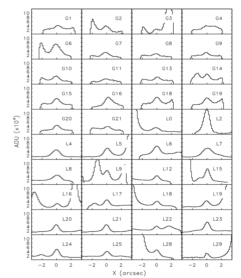
Figure 3.— The cross-sections of the slits of the objects obtained with LRIS and GMOS. The sections are displayed such that the white dwarf is in the center of the figure. The cross-sections of the LRIS objects were calculated from the first science exposure on July 15, 2007. This was the best exposure of our run in terms of seeing. The cross-sections of the GMOS objects were calculated from first science exposure taken of June 6, 2005.

The wavelength calibration was calculated from spectra of three lamps containing Hg, Zn, and Cd. There are not all that many transitions at these wavelengths, and furthermore, at the resolution we used, some of the lines had odd shapes. The residuals were not as well distributed as with the GMOS data, and the final dispersion of the wavelength residuals of the line fits was typically $\sim 0.1\,{\rm\AA}$. While there are not as many transitions as with the CuAr lamp used for the GMOS data, the wavelength solution is sufficiently precise for our purposes. The wavelength calibration was calculated with the identify task, and was applied to the science images with the dispcor task. The flux calibration for these stars was calculated from the flux standard HZ44, using the default values for the flux. The response was fix with a spline. The calibration was calculated using the tasks standard, and sensfunc, and were applied to the science spectra using the task calibrate. Finally, the individual spectra were combined using scombine, with the weights according to their signal-to-noise ratios.

Figure 4 shows the spectra that could be reliably extracted. While many of these spectra have too low a signal-to-noise ratio to determine masses, they all clearly show a Balmer series, and hence can be classified as type DA. The continuum play no role in the spectral classification, and has therefore simply been subtracted. Of the 35 slits observed between the GMOS and LRIS observations, 25 were strong white-dwarfs candidates. The other ten objects were included to fill the slit mask, but are unlikely to be white dwarfs. These objects were selected to be CV candidates, or white dwarf–main sequence star binary candidates. After preliminary reductions, none of these objects appeared to be interesting, and hence were not pursued further. All the strong candidates, except for one object (LRIS-27), have been confirmed to be type DA. We were unable to extract a reliable spectrum for LRIS-27 due to two other bright stars on the slit, and hence its spectral type is still unknown. For postage stamps of the area surrounding each target, see Kalirai et al. 2009.

Figure 4.— The spectra for all confirmed white dwarfs. Despite the low signal-to-noise ratio of some of these spectra, they are all clearly type DA. The expected position of H${10}$ through H$\beta$ are shown with dotted lines. The expected position of several helium lines (4026Å, 4388Å, 4471Å, 4922Å) are shown with dashed lines. None of the spectra show any significant lines at the positions of the helium lines. Note, the calcium K-line visible (between H$\varepsilon$ and H$8$) in objects L7 and L23 is most likely contamination due to very nearby main-sequence stars.

4. Discussion

4.1. Spectral Types

In total, we have determined the spectroscopic type of 24 white dwarfs. They are all of type DA. At this point it is of interest to take a closer look at the significance of this result. It is important for the following treatment that we be able to treat the observed white dwarfs as individual data points. The white dwarfs in our sample clearly all have the same metallicity and age, however, delaying discussion of these points to section 4.2, the cluster environment is unlikely to impart any other common property. Correlations of angular momentum, magnetic field, and rotation are all likely to be washed out during the formation of the cluster (Ménard and Duchêne, 2004). We can therefore treat the stars as individual data points.

We can use binomial statistics to determine the probability of observing no DB white dwarfs. The binomial distribution has the following form:

$$f(k;n)={n\choose k}p^{k}(1-p)^{n-k}$$ (1)

where $k$ is the number of observed events, $n$ is the number of trials, and $p$ is the probability of any one event giving a “positive result” (i.e., having a non-DA spectral type). When no events are observed, Equation 1 takes a particularly simple form:

$$f(0;n)=(1-p)^{n}$$ (2)

Under the assumption that the DA/DB ratio, $r$, is the same in the cluster environment as it is in the field, the probability of any one white dwarf being of type DB is:

$$p=\frac{1}{1+r}.$$ (3)

From SDSS-DR4, Eisenstein et al. (2006a) found $r\simeq 4.2$ for temperatures between $15\,000$–$25\,000$ K, implying $p=0.19$. Putting the preceding equations together, we have an expression for the probability, $f$, of observing no DB white dwarfs:

$$f(0;n)=(1-p)^{n}=0.81^{n}.$$ (4)

Assuming all 24 white dwarfs are cluster members, the probability of observing no DB white dwarfs is $6\times 10^{-3}$ ($2.5\sigma$ in a normal distribution). However, there is almost certainly a small level of contamination by field white dwarfs. Nine of the stars have their proper motions measured from WFPC2 astrometry. These stars are almost certainly cluster member. The probability of observing no DBs in this sub-sample is $0.15$ ($1.0\sigma$ in a normal distribution). An additional ten stars have photometry very close to the $0.5\,M_{\odot}$-cooling curve. If we include these, for a total of 19 cluster members, the probability of observing no DBs is $0.02$ ($2.1\sigma$ in a normal distribution). Of the remaining five stars, two (L8 and L22) have photometry marginally consistent with the white dwarf cooling sequence, while the other three (L2, L7, and L21) are unlikely to be cluster members. We will only include nineteen stars with cluster membership established by either proper motion or photometry in the following analysis.

We should also take into account the white dwarfs identified by Moehler et al. (2004). If we add the 9 white dwarfs identified by them in two other globular clusters, the total number of globular cluster identifications rises to 28. The chance of observing no DBs in a sample this large is only $3\times 10^{-3}$ ($2.8\sigma$ in a normal distribution). As a final note, Strickler et al. (2009) recently reported the discovery of 24 He-core white dwarfs in NGC 6397. These all show H$\alpha$ absorption, and are therefore likely all DAs. However, because these are photometric identifications, we will not consider these any further. It is now clear that the DA/DB ratio in globular clusters is different from that in the field.

Since 2005, a substantial number of white dwarfs in open clusters have had their spectral types determined. There are now a handful of non-DA white dwarfs identified. DBs have been found in NGC 6633 and NGC 6819 by Williams and Bolte (2007) and Kalirai et al. (2008) respectively. A DBA has been identified in the Hyades, and a DQ has been identified in NGC 2168 (Williams et al., 2006). It should be noted that none of the stars have their memberships confirmed by proper motions. However, assuming that all these stars are indeed genuine cluster members, we can calculate the probability of observing four or fewer non-DAs, $P(X\leq 4)$, in the total sample of $\sim 140$ stars:

$$P(X\leq 4)=\sum_{k=0}^{4}{140\choose k}(.19)^{k}(.81)^{140-k}=6\times 10^{-9},$$ (5)

the equivalent of a $5.7\sigma$ deviation in a normal distribution. It is now incontrovertible that the DA/DB ratio in the cluster environment is different from that in the field.

4.2. Possible Explanations

From the examination of cooling curves, and from the fitting of spectral lines (see Kalirai et al. 2009), we can constrain the effective temperatures of our stars to be cooler than $25\,000$ K. This is cool enough for He-convection to begin in white dwarfs with thin hydrogen envelopes, and would therefore transform at least a fraction of them to DBs. We can therefore use a hydrogen-rich atmosphere as a proxy for a thick hydrogen layer. The dearth of DB white dwarfs is more accurately thought of as a dearth of thin hydrogen envelopes. For the remainder of this section we will refer to white dwarfs with thick hydrogen envelopes as hydrogen rich (HR), those with thin hydrogen envelopes as hydrogen poor (HP).

At first blush, one may imagine many explanations that could explain the dearth of HP white dwarfs. However, many of these can be eliminated with several simple observations. The dearth of HP white dwarfs has now been observed in many open clusters and several globular clusters. These clusters cover a wide range of metallicity (from $-2.0<$[Fe/H]$<+0.4$), and we will therefore ignore any explanation that invokes metallicity. Furthermore, these clusters cover an extremely wide range of ages (from 100 Myr–12 Gyr), and therefore white-dwarf masses. The dearth of HP white dwarfs has been seen clearly in populations with average masses ranging from $M_{WD}\sim 0.8$ $M_{\odot}$ in open clusters (see Kalirai et al., 2005) to $M_{WD}\sim 0.5$ $M_{\odot}$ in globular clusters. These extreme populations comfortably bracket the peak of the mass distribution observed in the disk ($\bar{M}_{WD}=0.6$ $M_{\odot}$, see Bragaglia et al., 1995). We will therefore also ignore any explanation that invokes white dwarf mass. In the most general terms, we can propose explanations that either prevent the formation of HP white dwarfs, or transform the HP white dwarfs back to HR ones.

4.2.1 Suppression of HP formation

In order to prevent the formation of a HP white dwarf, we require a mechanism that will reduce the efficiency with which a star expels or burns its hydrogen envelope. One can imagine mechanisms involving binary stars that could affect the retention of a hydrogen envelope. There is evidence that the binary fraction in globular clusters is significantly lower than that of the field (Davis et al., 2008, and references therein). In particular, the binary fraction for extreme horizontal branch (EHB) stars is much lower in globular clusters than it is in the field (Moni Bidin et al., 2008). Castellani and Castellani (1993) showed that if sufficient mass is lost, a star can depart the red giant branch (RGB) before experiencing a helium core flash. These stars will experience the core flash later in their evolution and are referred to as “hot flashers”, and will be manifested as EHB stars in a globular cluster, or as sub-luminous O stars in the field. Lanz et al. (2004) showed that if the flash happens late enough during the star’s evolution, the energy of the flash can drive the expansion of the convection zone so that it engulfs the entire hydrogen envelope. This hydrogen will then be completely burned, and the resulting atmosphere will be completely dominated by helium.

If binaries drive mass loss, and increase the incidence of “hot flashers”, then higher binary fraction in the field may account for the increased incidence of HP white dwarfs there. However, only a small fraction of white dwarfs are formed from EHB stars, and not all of the EHB stars will be late hot flashers. This casts doubt upon the binary fraction/EHB channel as begin a likely explanation. Furthermore, the dearth of HP white dwarfs is also seen in open clusters, which have not been shown to have binary fractions significantly different from the field (see Kalirai and Tosi, 2004; Frinchaboy and Nielsen, 2008, for example). This casts doubt on the binary fraction in general being a feasible explanation.

Another possible avenue to lose mass might be very close encounters with other cluster members. The rate, $r$, of interactions within a given radius can be estimated as,

$$r=n\sigma v,$$ (6)

where $n$ is the number density of stars, $\sigma$ is the cross-section of interaction, and $v$ is the typical velocity of the interacting particles. For the mechanism to be successful, it requires a rate of at least one per typical RGB-star lifetime, which is assumed to be $t\simeq t_{RGB}=350$ Myr. An interaction that liberates a significant mass of gas from a RGB star will have a radius comparable to several times the radius of the star, which is approximately $R\simeq R_{RGB}=1$ AU. Finally, we assume a velocity that is in line with a typical velocity dispersion of a star cluster, i.e., $v\simeq v_{5}=5\,km/s$.

Rearranging Equation 6, we can estimate the necessary density for one interaction to occur within the lifetime of a RGB star

$$n=5\times 10^{5}\,pc^{-3}\,\,\left(\frac{t}{t_{RGB}}\right)^{-1}\left(\frac{R}{R_{RGB}}\right)^{-2}\left(\frac{v}{v_{5}}\right)^{-1}$$ (7)

This density is higher than is present in most, if not all, globular clusters, and far higher than the majority of open clusters, and is hence unlikely to be a feasible explanation.

4.2.2 Transformation of HP to HR

Transforming an HP white dwarf to a HR white dwarf simply requires the star to re-accrete a hydrogen envelope. A re-accreted hydrogen layer can either suppress convection in the helium layer or, if it is thick enough, resist being drawn into the interior of the star completely when convection does occur. It is unclear what the absolute minimum mass of hydrogen necessary for this, however, we can get a lower limit by examining the accretion rate of white dwarfs in the field. The Bondi accretion rate is

$$\dot{M}=\frac{4\pi m_{p}nG^{2}M^{2}}{V^{3}},$$ (8)

where $M$ is the mass of the star, $V$ is the relative velocity of the gas and the star, $n$ is the number density of protons, and $m_{p}$ is the mass of the proton. Substituting typical values for a disk white dwarf, we have

$$\dot{M}=5\times 10^{-17}\,M_{\odot}/yr\,\frac{M^{2}_{WD}\,n_{ISM}}{\,V^{3}_{30}},$$ (9)

where $M_{WD}=0.5\,M_{\odot}$, $n_{ISM}=1\,cm^{-3}$, and $V_{30}=30\,km/s$. The stars we are examining have cooling time of approximately $20$ Myr, and hence we would expect the average field white dwarf at a temperature similar to the white dwarfs observed in M4 to have accreted approximately $10^{-9}\,M_{\odot}$ of hydrogen from the ISM. We assume a lower limit to transform a DB to a DA is an order of magnitude greater than this, i.e., $M_{min}=10^{-8}\,M_{\odot}$, or equivalently $\dot{M}_{min}=5\times 10^{-16}\,M_{\odot}/yr$, or finally, $n_{min}=10\,cm^{-3}$.While we do not yet have a definitive scenario that can increase the accretion rate to the requisite level, we will briefly examine two possibilities: accretion from a central reservoir of gas, and accretion from the cluster wind (i.e., the composite wind from all stars).

An obvious way to increase the density of the intra-cluster medium, and therefore the accretion rate of the cluster white dwarfs, is accretion of gas into the cluster potential. Lin and Murray (2007) explore the accretion of gas into the gravitational potentials of star clusters, and the subsequent effect on accretion rates of individual stars. The efficiency at which a cluster can accrete gas is determined primarily by the relative velocities of the cluster compared with the ISM. Most globular clusters move at velocities relative to the ISM of $\sim 10^{2}\,km/s$ with respect to the ISM, and will not effectively accrete gas.

As the relative velocity of the cluster and ISM drops below the velocity dispersion of the cluster, the cluster potential starts to accrete gas, and dramatically increases the accretion rate of the individual stars. The estimated rate for a globular cluster with a velocity dispersion of $10\,km/s$, according to Lin and Murray (2007), is $10^{-13}\,M_{\odot}/yr$. This rate is well above the required rate. However, the fact that most globular clusters (including M4, NGC6397, and NGC6752, i.e.  all the globular clusters that have had spectral observations reported) have velocities well above this velocity, makes this an unlikely explanation for the observed effect. Furthermore, the shallow potential of open cluster makes this an unlikely scenario in that environment too.

Another source of gas could be the collective winds of the other stars in the cluster. The winds from evolved low- and intermediate-mass stars have typical velocities of $10$–$30\,km\,s^{-1}$ and hence we would not expect the gas to be retained by the gravitational potential of most clusters. The accretion would therefore be from a smooth cluster wind. This scenario was explored for the open cluster NGC 2099 in Kalirai et al. (2005), and found to be an unlikely explanation. Following their analysis, we present a more general expression for the accretion rate due to a cluster wind.

In order to estimate the density of the cluster wind, we make several assumptions. First, we assume the cluster has a Salpeter mass function from $0.1$–$8.0\,M_{\odot}$, the upper limit being the approximate limit at which white dwarfs will form. We determine an expression for the turn-off mass, $M_{TO}$, as a function of time by examining the models of Dotter et al. (2006). We find a satisfactory fit with

$$M_{TO}=1.633\left(\frac{t}{1\,{\rm Gyr}}\right)^{-0.2935}.$$ (10)

In order to determine the mass loss per star, we subtract the remnant mass as determined in Kalirai et al. (2009) from $M_{TO}$. The mass returned to the ISM, $M_{ISM}$, is

$$M_{ISM}=0.89\,M_{TO}-0.39\,M_{\odot}.$$ (11)

The lifetime of a main sequence star combined with the IMF tells us the number of stars evolving off the main sequence as a function of time. Each star leaving the main sequence returns a certain mass of gas back to the ISM, and therefore the total mass begin returned to the ISM as a function of time can be calculated. Assuming the cluster retains none of this gas, this is equivalent to the mass loss from the cluster. Unfortunately, due to the form of Equations 10 and 11 this could not be done analytically. The numerical result was well approximated by the following expression for mass loss from a cluster due to the composite stellar wind in units of $M_{\odot}/yr$,

$$\dot{M}_{cl}=1.22\times 10^{-7}\,\left(\frac{M_{cl}}{10^{4}M_{\odot}}\right)\left(\frac{t+1.1}{1\,Gyr}\right)^{-1.17}.$$ (12)

Of course, not all the stars returning gas to the ISM are at the center of the cluster, but due to mass segregation the most massive star will be the most centrally concentrated. The approximation that all the mass loss occurs at the center of the cluster is good enough for our purposes. The gas density due to the cluster wind at a radius $R$ from the cluster center will be

$$n=1.0\times 10^{-3}\,cm^{-3}\left(\frac{3\,pc}{R}\right)^{2}\frac{\dot{M}_{cl}(t)}{\dot{M}_{cl}(1\,Gyr)}.$$ (13)

This density is far below the critical density necessary for accretion to transform HP to HR white dwarfs, and is in fact less than the mean density of the ISM, and hence can be neglected.

This treatment of mass loss and accretion has been rather crude. We assumed that the gas leaves the cluster in a smooth way. Perhaps the winds from different stars interact in a way that causes them to cool, and be retained by the cluster more efficiently than one would naïvely expect.

5. Conclusion

With an additional 24 white-dwarf spectral-type identifications, we have roughly tripled the number of spectral identifications in globular clusters. All the newly identified white dwarfs are DAs. This extends the already-observed phenomenon of star clusters being deficient in non-DA white dwarfs to cover essentially all metallicities and white-dwarf masses. It is now incontrovertible that the DA/DB ratio is different in the field than in the cluster environment.

The discovery of a handful of non-DA white dwarfs in several open clusters show that is not impossible to form a non-DA white dwarf in the cluster environment, however, the formation mechanism is clearly strongly suppressed. Unfortunately, there is no obvious mechanism for this, but it seems likely that some mechanism exists that enables the re-accretion of a hydrogen envelope. The dearth of non-DA white dwarfs in clusters relative to the field has now been clearly demonstrated across the full range of age and metallicity, and remains an unsolved problem in stellar evolution.

Facilities: Gemini:South (GMOS), HST (WFPC2), Keck:I (LRIS)

References

- Bergeron et al. [1997] P. Bergeron, M. T. Ruiz, and S. K. Leggett. The Chemical Evolution of Cool White Dwarfs and the Age of the Local Galactic Disk. ApJS, 108:339, January 1997. 10.1086/312955.
- Bragaglia et al. [1995] A. Bragaglia, A. Renzini, and P. Bergeron. Temperatures, gravities, and masses for a sample of bright DA white dwarfs and the initial-to-final mass relation. ApJ, 443:735–752, April 1995. 10.1086/175564.
- Castellani and Castellani [1993] M. Castellani and V. Castellani. Mass loss in globular cluster red giants - an evolutionary investigation. ApJ, 407:649–656, April 1993. 10.1086/172547.
- Davis et al. [2008] D. S. Davis, H. B. Richer, J. Anderson, J. Brewer, J. Hurley, J. S. Kalirai, R. M. Rich, and P. B. Stetson. Deep Advanced Camera for Surveys Imaging in the Globular Cluster NGC 6397: the Binary Fraction. AJ, 135:2155–2162, June 2008. 10.1088/0004-6256/135/6/2155.
- Dotter et al. [2006] A. L. Dotter, B. Chaboyer, E. Baron, J. W. Ferguson, D. Jevremovic, H. Lee, and G. Worthey. Self-Consistent Stellar Evolution Models with Updated Physics and Variable Abundances. In Bulletin of the American Astronomical Society, volume 38 of Bulletin of the American Astronomical Society, pages 958, December 2006.
- Eisenstein et al. [2006a] D. J. Eisenstein, J. Liebert, H. C. Harris, S. J. Kleinman, A. Nitta, N. Silvestri, S. A. Anderson, J. C. Barentine, H. J. Brewington, J. Brinkmann, M. Harvanek, J. Krzesiński, E. H. Neilsen, Jr., D. Long, D. P. Schneider, and S. A. Snedden. A Catalog of Spectroscopically Confirmed White Dwarfs from the Sloan Digital Sky Survey Data Release 4. ApJS, 167:40–58, November 2006a. 10.1086/507110.
- Eisenstein et al. [2006b] D. J. Eisenstein, J. Liebert, D. Koester, S. J. Kleinmann, A. Nitta, P. S. Smith, J. C. Barentine, H. J. Brewington, J. Brinkmann, M. Harvanek, J. Krzesiński, E. H. Neilsen, Jr., D. Long, D. P. Schneider, and S. A. Snedden. Hot DB White Dwarfs from the Sloan Digital Sky Survey. AJ, 132:676–691, August 2006b. 10.1086/504424.
- Fontaine et al. [2001] G. Fontaine, P. Brassard, and P. Bergeron. The Potential of White Dwarf Cosmochronology. PASP, 113:409–435, April 2001.
- Frinchaboy and Nielsen [2008] P. M. Frinchaboy and D. Nielsen. The WIYN Open Cluster Study Photometric Binary Survey: Initial Findings for NGC 188. In E. Vesperini, M. Giersz, and A. Sills, editors, IAU Symposium, volume 246 of IAU Symposium, pages 109–110, May 2008. 10.1017/S174392130801541X.