Analog control of open quantum systems under arbitrary decoherence

Abstract

We derive and investigate a general non-Markovian equation for the time-dependence of a Hamiltonian that maximizes the fidelity of a desired quantum gate on any finite-dimensional quantum system in the presence of arbitrary bath and noise sources. The method is illustrated for a single-qubit gate implemented on a three-level system.

I Introduction

The quest for strategies for combatting decoherence is of paramount importance to the control of open quantum systems, particularly for quantum information operations Nielsen and Chuang (2000). A prevailing unitary strategy aimed at suppressing decoherence is dynamical decoupling (DD) Viola and Lloyd (1998); Khodjasteh and Lidar (2005); Uhrig (2007), which consists, in the case of a qubit, in the application of strong and fast pulses alternating along orthogonal Bloch-sphere axes, e.g., $X$ and $Z$. In the frequency domain, where the decoherence rate can be described as overlap between the spectra of the pulse-driven (modulated) system and the bath Kofman and Kurizki (2001), DD is tantamount to shifting the driven-system resonances beyond the bath cutoff frequencies. The DD efficacy can be enhanced for certain bath spectra upon choosing the timings of the pulses so as to reduce the low-frequency parts in the system spectrum and thus its overlap with the low-frequency portion of the bath spectrum Uhrig (2007). DD sequences are inherently binary, i.e., their pulsed control parameters are discretely switched on or off. Realistically, the finiteness of pulse durations and spacings sets an upper limit on the speed and fidelity of DD-assisted quantum gate operations Viola and Lloyd (1998); Khodjasteh and Lidar (2005); Uhrig (2007).

An alternative strategy formulated here in full generality is analog unitary control of multidimensional systems subject to any noise or decoherence. It is effected by a system Hamiltonian whose time-dependence is variationally tailored to optimally perform a desired gate operation. The vast additional freedom of non-discrete (smooth) Hamiltonian parametrization significantly enhances the efficacy of decoherence control under realistic constraints compatible with the non-Markov time scales required for such control. Its formulation meets the long-standing conceptual challenge of simultaneously controlling non-commuting system operators subject to noise along orthogonal axes. This is here achieved by working in an optimally rotated, different basis at each instant. The price we pay for such general optimal control is the need for at least partial knowledge of the bath or noise spectrum, which is experimentally accessible Sagi et al. (2009) without the need for microscopic models. The goal is to minimize its overlap with the spectrum of the controlled system, as was already shown for pure dephasing of qubits Gordon et al. (2008).

II Gate Error

We assume that the system Hamiltonian $\hat{H}_{\mathrm{S}}(t)$ implements a desired quantum gate operation at time $t$, and aim at designing it so as to minimize the decoherence and noise errors. The system-bath interaction $\hat{H}_{\mathrm{I}}$ then acquires time-dependence in the interaction picture under the action of $\hat{H}_{\mathrm{S}}(t)$ and the bath Hamiltonian $\hat{H}_{\mathrm{B}}$. Assuming factorized initial states of the system and the bath, $\hat{\varrho}_{\mathrm{tot}}(0)$ $\!=$ $\!\hat{\varrho}(0)\otimes\hat{\varrho}_{\mathrm{B}}$, tracing over the bath, and further assuming that $\mathrm{Tr}_{\mathrm{B}}[\hat{H}_{\mathrm{I}}(t)\hat{\varrho}_{\mathrm{B}}]$ $\!=$ $\!\hat{0}$, yields for the system state $\hat{\varrho}(t)$ the integrated (exact) deviation from the initial state (App.A),

$$\hat{\varrho}(t) = \!\hat{\varrho}(0)-\Delta\hat{\varrho}(t),$$

$$\Delta\hat{\varrho}(t) = \!\!\int_{0}^{t}\!\!\!\mathrm{d}t_{1}\!\int_{0}^{t_{1}}\!\!\!\mathrm{d}t_{2}\mathrm{Tr}_{\mathrm{B}}[\hat{H}_{\mathrm{I}}(t_{1}),[\hat{H}_{\mathrm{I}}(t_{2}),\hat{\varrho}_{\mathrm{tot}}(t_{2})]].\quad$$ (1)

In what follows, we assume that up to $t$, the combined system-bath state changes only weakly compared to $\hat{H}_{\mathrm{I}}$, so that we approximate in (1) $\hat{\varrho}_{\mathrm{tot}}(t_{2})\approx\hat{\varrho}_{\mathrm{tot}}(0)$ in the integral. This means that the control is assumed effective enough to allow only small errors, consistently with the first order approximation of the solutions of both the Nakajima-Zwanzig and the time-convolutionless master equations Gordon et al. (2007); Breuer and Petruccione (2002).

To justify this assumption, we try to reduce the discrepancy between the states evolved for time $t$ in the presence and absence of the bath by minimizing $\langle\Delta\hat{\varrho}(t)\rangle$ $\!\equiv$ $\!\langle\Psi|\Delta\hat{\varrho}(t)|\Psi\rangle$ averaged over all initial states $|\Psi\rangle$ that are unknown in general. For a $d$-level system this averaging is tantamount to taking the expectation value with respect to the maximum entropy state $\hat{\varrho}_{\mathrm{S}}$ $\!=$ $\!d^{-1}\hat{I}$. Assuming that $\mathrm{Tr}_{\mathrm{S}}[\hat{H}_{\mathrm{I}}(t)\hat{\varrho}_{\mathrm{S}}]$ $\!=$ $\!\hat{0}$, we obtain our measure of decoherence (error) in the form of (App.A)

$$\overline{\langle\Delta\hat{\varrho}(t)\rangle} = \!2\kappa\mathrm{Re}\!\int_{0}^{t}\!\mathrm{d}t_{1}\!\int_{0}^{t_{1}}\!\mathrm{d}t_{2}\bigl{\langle}\hat{H}_{\mathrm{I}}(t_{1})\hat{H}_{\mathrm{I}}(t_{2})\bigr{\rangle}_{\mathrm{SB}}$$ (2)

$$= \kappa\Bigl{\langle}\Bigl{[}\int_{0}^{t}\!\mathrm{d}t_{1}\hat{H}_{\mathrm{I}}(t_{1})\Bigr{]}^{2}\Bigr{\rangle}_{\mathrm{SB}},$$

where $\kappa$ $\!=$ $\!1\!-\!(d\!+\!1)^{-1}$, $\langle\cdot\rangle_{\mathrm{SB}}$ $\!=$ $\!\mathrm{Tr}_{\mathrm{SB}}[(\cdot)\hat{\varrho}_{\mathrm{S}}\otimes\hat{\varrho}_{\mathrm{B}}]$. Hence, $\overline{\langle\Delta\hat{\varrho}(t)\rangle}$ is always positive and proportional to the mean square of the interaction energy as observed in the interaction picture (by a co-rotating observer).

Since our aim is to suppress $\overline{\langle\Delta\hat{\varrho}(t)\rangle}$ by system manipulations alone, we now separate system and bath parts by decomposing any interaction Hamiltonian in an orthogonal basis of system states $|j\rangle$ as

$$\hat{H}_{\mathrm{I}}(t)=\sum_{j=1}^{d^{2}-1}\hat{B}_{j}(t)\hat{S}_{j}(t),$$ (3)

where the Hermitian $\hat{B}_{j}$ and $\hat{S}_{j}$ are bath and system operators, respectively, assumed to obey $\langle\hat{B}_{j}(t)\rangle_{\mathrm{B}}$ $\!=$ $\!\mathrm{Tr}\hat{S}_{j}(t)$ $\!=$ $\!0$ and carry no explicit time dependence. In the interaction picture

$$\hat{B}_{j}(t) = \mathrm{e}^{\mathrm{i}\hat{H}_{\mathrm{B}}t}\hat{B}_{j}\mathrm{e}^{-\mathrm{i}\hat{H}_{\mathrm{B}}t},$$

$$\hat{S}_{j}(t) = \hat{U}^{\dagger}(t)\hat{S}_{j}\hat{U}(t),$$

$$\hat{U}(t) = \mathrm{T}_{+}\mathrm{e}^{-\mathrm{i}\int_{0}^{t}\!\mathrm{d}t^{\prime}\hat{H}_{\mathrm{S}}(t^{\prime})}.$$ (4)

We shall minimize $\overline{\langle\Delta\hat{\varrho}(t)\rangle}$ for given, experimentally accessible Sagi et al. (2009), bath correlations

$${\Phi}_{jk}(t)=\bigl{\langle}\hat{B}_{j}(t)\hat{B}_{k}\bigr{\rangle}_{\mathrm{B}}.$$ (5)

It is expedient to define the decoherence matrix

$$\underline{\bm{R}}(t_{1},t_{2})=\underline{\bm{\epsilon}}^{T}(t_{1})\underline{\bm{\Phi}}(t_{1}-t_{2})\underline{\bm{\epsilon}}(t_{2}),$$ (6)

which obeys $\underline{\bm{R}}^{\dagger}(t_{1},t_{2})$ $\!=$ $\!\underline{\bm{R}}(t_{2},t_{1})$. It is the matrix product of the bath correlation matrix $\underline{\bm{\Phi}}$ formed from the coefficients ${\Phi}_{jk}$ in (5) and the system-modulation (rotation) matrix defined as

$$\hat{S}_{j}(t) = \sum_{k=1}^{d^{2}-1}{\epsilon}_{jk}(t)\hat{S}_{k},$$

$$\quad{\epsilon}_{jk}(t) = \frac{1}{2}\mathrm{Tr}[\hat{S}_{j}(t)\hat{S}_{k}],$$ (7)

where we have assumed that $\mathrm{Tr}(\hat{S}_{j}\hat{S}_{k})$ $\!=$ $\!2\delta_{jk}$. The transformation (7) is at the heart of the treatment: it defines the instantaneous rotating frame where the system and bath are maximally decoupled, as shown below.

We can now write (2) as (App.B)

$$\overline{\langle\Delta\hat{\varrho}(t)\rangle}=2\frac{\kappa}{d}\;\int_{0}^{t}\!\mathrm{d}t_{1}\int_{0}^{t}\!\mathrm{d}t_{2}\mathrm{Tr}\underline{\bm{R}}(t_{1},t_{2}).$$ (8)

Alternatively, we can rewrite (8) as

$$\overline{\langle\Delta\hat{\varrho}(t)\rangle}=4t\,\frac{\kappa}{d}\int_{0}^{\infty}\mathrm{d}\omega\,\mathrm{Tr}[\underline{\bm{G}}(\omega)\underline{\bm{F}_{t}}(\omega)],$$ (9)

i.e., as the spectral overlap of two matrix-valued functions: the bath coupling spectral matrix $\underline{\bm{G}}(\omega)$ $\!=$ $\!\int_{-\infty}^{\infty}\!\mathrm{d}t\;\mathrm{e}^{\mathrm{i}\omega{t}}\;\mathrm{Re}\underline{\bm{\Phi}}(t)$, and the system-modulation spectral matrix at finite time $t$ [cf. (6)] $\underline{\bm{F}_{t}}(\omega)$ $\!=$ $\!\frac{1}{t}\underline{\bm{\epsilon}_{t}}(\omega)\underline{\bm{\epsilon}_{t}}^{\dagger}(\omega)$, $\underline{\bm{\epsilon}_{t}}(\omega)$ $\!=$ $\!\frac{1}{\sqrt{2\pi}}\int_{0}^{t}\mathrm{d}\tau\,\mathrm{e}^{\mathrm{i}\omega\tau}\underline{\bm{\epsilon}}(\tau)$. In (9) we have made use of the fact that $\underline{\bm{\Phi}}(-t)$ $\!=$ $\!\underline{\bm{\Phi}}^{\dagger}(t)$, so that it is sufficient to integrate over positive frequencies.

Equation (9) constitutes a generalization of the “universal formula” Kofman and Kurizki (2001) to arbitrary multidimensional systems and baths. It provides a major insight: the system and bath spectra (all matrix components) must be anticorrelated, i.e., ${G}_{jk}(\omega)$ minima must coincide with $({F}_{t})_{jk}(\omega)$ maxima and vice versa to minimize (9), as illustrated below. It should be emphasized that for given $\omega$, both $\underline{\bm{G}}(\omega)$ and $\underline{\bm{F}_{t}}(\omega)$ are positive matrices. Nevertheless, certain components ${G}_{jk}(\omega)$, $({F}_{t})_{jk}(\omega)$ may be negative if $d$ $\!>$ $\!2$ (i.e., not for qubits). This may allow us to ‘destructively interfere’ their contributions, i.e., engineer “dark states” Gordon and Kurizki (2006) or “decoherence-free” subspaces Wu et al. (2005). These prospects of our general scheme will be explored elsewhere.

III Decoherence Minimization

Our goal is to find a system Hamiltonian $\hat{H}_{\mathrm{S}}({t_{1}})$, $0$ $\!\leq$ $\!t_{1}$ $\!\leq$ $\!t$, implementing a given unitary gate $\hat{U}(t)$ at a fixed time $t$ according to (4). This requires minimizing (2) or (8), $\overline{\langle\Delta\hat{\varrho}(t)\rangle}$ $\!\to$ $\!{min}$, i.e., minimizing the bath-induced state error in the interaction picture under $\hat{H}_{\mathrm{S}}(t)$. We may similarly account for the effects of modulation or control noise, in addition to bath noise (App.C).

The major difficulty in minimizing (8) using (4)-(7) is that (4) involves time-ordered integration for arbitrary bath and control axes. To circumvent this difficulty, we make use of $\hat{U}(t_{1})$ instead of $\hat{H}_{\mathrm{S}}$, and assume a parametrization $\hat{U}[{f}_{l}({t_{1}}),{t_{1}}]$ in terms of a set of real parameters ${{f}}_{l}({t_{1}})$, which may be combined to a vector $\underline{\bm{{f}}}({t_{1}})$. The number of parameters may vary, since the parametrization does not have to be complete. The boundary values $\underline{\bm{{f}}}(0)$ and $\underline{\bm{{f}}}(t)$ should be such that $\hat{U}(t_{1}\!=\!0)$ $\!=$ $\!\hat{I}$ and $\hat{U}(t_{1}\!=\!t)$ is the desired gate.

If a bath coupling spectrum $\underline{\bm{G}}(\omega)$ vanishes (has cutoff) at any high frequency, the overlap (9) can be presumed arbitrarily small under sufficiently rapid modulation of the Hamiltonian, such that all components of $\underline{\bm{F}_{t}}(\omega)$ are shifted beyond this cutoff, thus achieving DD Viola and Lloyd (1998); Khodjasteh and Lidar (2005); Uhrig (2007). Yet this may require a diverging system energy. Furthermore, fidelity generally drops with modulation energy, as discussed below. We therefore impose an energy constraint on the modulated system

$$E_{\mathrm{S}}=\int_{0}^{t}\!\mathrm{d}{t_{1}}\bigl{\langle}\hat{H}_{\mathrm{S}}^{2}({t_{1}})\bigr{\rangle}_{\mathrm{S}}={const}.,$$ (10)

where $\langle\cdot\rangle_{\mathrm{S}}$ $\!=$ $\!\mathrm{Tr}[(\cdot){d}^{-1}\hat{I}]$ [cf. (2)]. An alternative constraint

$$E=\int_{0}^{t}\mathrm{d}{t_{1}}\;|\dot{\underline{\bm{{f}}}}({t_{1}})|^{2}={const}.$$ (11)

allows a simplified treatment. In general, $E$ accounts for the fact that the time dependence of a parametrization cannot be arbitrarily fast and hence bounds the modulated $\hat{H}_{\mathrm{S}}({t_{1}})$, thus also limiting $E_{\mathrm{S}}$.

The minimization of (8) subject to (11) is an extremal problem in terms of $\underline{\bm{{f}}}$. Denoting by $\underline{\bm{\delta}}$ the total variation with respect to $\underline{\bm{{f}}}$, the stationary condition can be formulated in terms of a Lagrange multiplier $\lambda$ as $\underline{\bm{\delta}}\overline{\langle\Delta\hat{\varrho}(t)\rangle}$ $\!+$ $\!\lambda\underline{\bm{\delta}}E$ $\!=$ $\!0$. Then, using the parametrization in $\underline{\bm{R}}$ [Eq. (6)], $\nabla\underline{\bm{\epsilon}}$ $\!\equiv$ $\!\{\frac{\partial}{\partial{{f}}_{l}}\underline{\bm{\epsilon}}(t_{1})\}$, yields the Euler-Lagrange equation

$$\ddot{\underline{\bm{{f}}}}(t_{1})=\lambda\underline{\bm{{g}}}(t_{1}),\quad\underline{\bm{{g}}}(t_{1})\equiv\int_{0}^{t}\!\mathrm{d}t_{2}\nabla\mathrm{Re}\mathrm{Tr}\underline{\bm{R}}(t_{1},t_{2}),$$ (12)

where $\lambda$ is related to the constraint (11) on $E$ (App.D).

We conclude the general treatment by recapitulating on the steps to find the optimal modulation of $\hat{H}_{\mathrm{S}}({t_{1}})$: 1) After defining the ‘cycle time’ $t$ and gate operation $\hat{U}(t)$, we declare a parametrization $\hat{U}[\underline{\bm{{f}}}({t_{1}}),{t_{1}}]$ which induces a parametrization $\underline{\bm{\epsilon}}[\underline{\bm{{f}}}({t_{1}}),{t_{1}}]$ that in turn yields $\underline{\bm{R}}(t_{1},t_{2})$ as a functional of $\underline{\bm{{f}}}$ via (4)-(7), using our knowledge of (5). 2) We now solve (12) for a given initial $\underline{\bm{{f}}}_{\mathrm{init}}(t_{1})$ satisfying the boundary conditions, e.g., such that $\hat{U}[\underline{\bm{{f}}}_{\mathrm{init}}(t_{1}),{t_{1}}]$ $\!=$ $\![\hat{U}(t)]^{\frac{t_{1}}{t}}$, and calculate $\overline{\langle\Delta\hat{\varrho}(t)\rangle}$. 3) The optimization is repeated for different values of $\lambda$ and $E_{\mathrm{S}}$ in (10) is calculated for each solution. Among all solutions for which $\overline{\langle\Delta\hat{\varrho}(t)\rangle}$ falls below a desired threshold value, we choose the one corresponding to the lowest $E_{\mathrm{S}}$. 4) The chosen solution $\underline{\bm{{f}}}({t_{1}})$ is inserted into $\hat{U}[\underline{\bm{{f}}}({t_{1}}),{t_{1}}]$ in (4), yielding the instantaneous control parameters

$$\hat{H}_{\mathrm{S}}({t_{1}})=\sum_{j}\omega_{j}({t_{1}})\hat{S}_{j},\quad\omega_{j}({t_{1}})=\frac{1}{2}\mathrm{Tr}[\hat{S}_{j}\hat{H}_{\mathrm{S}}({t_{1}})].$$ (13)

IV Application to a qubit

To apply the general procedure to a qubit for which $\hat{S}_{j}$ $\!=$ $\!\hat{\sigma}_{j}$ ($j$ $\!=$ $\!x,y,z$) in (13), we resort to the Euler rotation-angle parametrization,

$$\hat{U}(t)=\mathrm{e}^{-\frac{\mathrm{i}}{2}f_{3}(t)\hat{\sigma}_{3}}\mathrm{e}^{-\frac{\mathrm{i}}{2}f_{2}(t)\hat{\sigma}_{2}}\mathrm{e}^{-\frac{\mathrm{i}}{2}f_{1}(t)\hat{\sigma}_{3}}.$$

In (13), $\omega_{3}(t)$ is now the level splitting, whereas $\omega_{1(2)}(t)$ are Rabi flipping rates. We choose two examples of uncorrelated (i.e., diagonal) baths, namely, an Ohmic bath with different cutoffs in $X$, $Y$, $Z$, and a Lorentzian noise spectrum superposed with a second Lorentzian such that a spectral ‘hole’ is obtained at different frequencies in $X$, $Y$, and $Z$. The corresponding bath coupling spectra are shown in Fig. 1, along with our optimized modulation spectra, which are contrasted with Uhrig’s DD pulse-sequence spectra Uhrig (2007) (App.E,F).

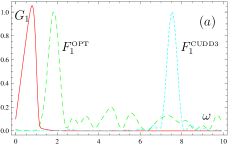
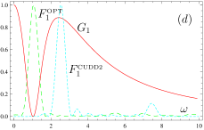
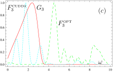
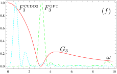
Figure 1: Spectral overlaps between bath spectra $G_{i}(\omega)$ (solid red), modulation spectra $F_{i}^{\scriptscriptstyle{\mathrm{OPT}}}(\omega)$ (dashed green) for an optimized $\pi$-gate at $E_{\mathrm{S}}$ $\!=$ $\!133.2$ [(a),(b),(c)], and an optimized identity ($0$-) gate at $E_{\mathrm{S}}$ $\!=$ $\!181.1$ [(d),(e),(f)], respectively, and modulation spectra $F_{i}^{\scriptscriptstyle{\mathrm{CUDD}}}$ for pulse sequences (App.F) CUDD3 [(a),(b),(c)] and CUDD2 [(d),(e),(f)] (dotted blue), with $i=1,2,3$ corresponding to $X$, $Y$, and $Z$-component, respectively. Graphs (a),(b),(c) represent an Ohmic bath spectrum with softened cutoff, whereas graphs (d),(e),(f) represent a Lorentzian spectrum with a dip. The optimal modulation spectra $F_{i}^{\scriptscriptstyle{\mathrm{OPT}}}(\omega)$ are always anticorrelated with the bath spectra $G_{i}(\omega)$. By contrast, Uhrig’s pulse sequence spectra $F_{i}^{\scriptscriptstyle{\mathrm{CUDD}}}$ are only anticorrelated with $G_{i}$ for Ohmic baths (a),(b) but not for the bath spectra (d),(e),(f).

The minimized gate error is shown in Fig. 2 as a function of the energy constraint (10) for both baths.

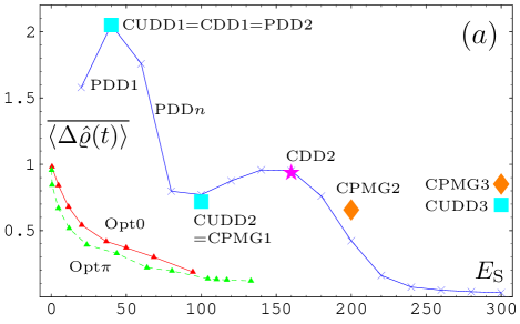
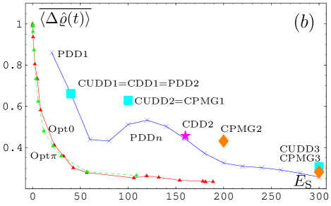
Figure 2: Qubit gate error $\overline{\langle\Delta\hat{\varrho}(t)\rangle}$ in units of a reference $\overline{\langle\Delta\hat{\varrho}(t)\rangle}_{\mathrm{ref}}$ which corresponds to a time-independent initial system Hamiltonian (with which the optimization started), as a function of the constraint $E_{\mathrm{S}}$. Solid red (dashed green): optimized identity ($\pi$)-gate, Solid blue: periodic $X$-$Z$-“bang bang” (2,4,$\ldots$,30 pulses). Separate points: concatenated Uhrig and related pulse sequences (App.F). (a) and (b) correspond to bath spectra shown on the left and right in Fig. 1. A different scale of $E_{\mathrm{S}}$ is used for pulse sequences whose $E_{\mathrm{S}}$ is given in units of $E_{\mathrm{S}}^{(1)}/10$, where $E_{\mathrm{S}}^{(1)}$ $\!=$ $\!\pi^{2}/(4T)=2.467\cdot 10^{3}$ is the single $\pi$-pulse energy, assuming nearly-ideal square pulses.

Its comparison with the gate error obtained using various DD pulse sequences reveals two differences. The first concerns the energy scale: in rectangular DD pulse sequences, each $\pi$-pulse of duration $T$ contributes an amount $\pi^{2}/(4T)$ to (10), which diverges for ideal pulses, $T$ $\!\to$ $\!0$. By contrast, our approach assumes finite, much smaller $E_{\mathrm{S}}$. The second difference concerns energy monotonicity: DD-sequences are designed a priori, regardless of the bath-spectrum, and hence only significantly reduce the gate error if $E_{\mathrm{S}}$ has risen above some threshold which is needed to shift all system frequencies beyond the bath cutoffs Uhrig (2007). In contrast, our approach starts to reduce the gate error as soon as $E_{\mathrm{S}}$ $\!>$ $\!0$, since it optimizes the use of the available energy, by anti-correlating the modulation and bath spectra.

We next consider the gate fidelity limitations as a function of $E_{S}$ posed by leakage Wu et al. (2009) to levels outside the relevant subspace (here a qubit). In a 3-level $\Lambda$-system, any off-resonant control field acting on the qubit levels $|1\rangle$, $|2\rangle$, causes leakage to the unwanted level $|3\rangle$ Agarwal (1996). Such leakage and the ensuing incoherent decay $|3\rangle$ $\!\to$ $\!|1\rangle$ incur gate errors that grow with $E_{\mathrm{S}}$ (App.G). This behaviour is illustrated in Fig. 3, which reveals that leakage error is the more dramatic, the more energetic the $\pi$-pulse sequences are. If $\pi$-pulses are experimentally implemented as $(2m+1)\pi$-pulses, $m{\scriptstyle\gtrapprox}10^{3}$, it can therefore be expected that isolated manipulation on a subspace is difficult. This, together with the qubit-gate optimization, the general expressions for the gate error (8) and (9) and its minimization (12) are the main results of this work.

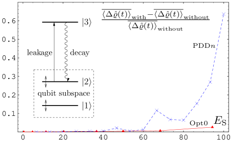
Figure 3: Relative surplus error incurred by the inevitable leakage to the additional level $|3\rangle$ (inset) caused by control $f(t)$ as a function of $E_{\mathrm{S}}$, i.e., error with allowance for leakage compared to the error without (disregarding) leakage (App.G). Solid red: optimized identity-gate, dashed blue: periodic $X$-$Z$-“bang bang” (2,4,$\ldots$,30 pulses) as shown in Fig. 2(a) and a bath spectrum as shown in Fig. 1(a),(b),(c). A (truncated) $1/\omega$ bath coupling spectrum describes an amplitude coupling between levels $|2\rangle$ and $|3\rangle$ (leakage). As in Fig. 2, a different scale of $E_{\mathrm{S}}$ is used for the pulse sequences: $E_{\mathrm{S}}$ is here given in units of $(3/10)E_{\mathrm{S}}^{(1)}$.

V Conclusions

A) We have expressed an arbitrary gate error for finite-dimensional quantum systems as the spectral overlap between the driven-system and the bath spectra. B) We have derived a non-Markovian Euler-Lagrange equation for the time dependence of control parameters whose solution maximizes the gate fidelity. C) This solution leads to anticorrelation of the system and bath spectra. Hence, while DD-based methods rely on shifting the entire spectrum of the system beyond that of the bath, our optimization takes advantage of gaps or dips of the bath spectra. D) The treatment of a qubit demonstrates that our approach is significantly more economic in terms of energy investment than DD-based methods. Such energy saving may be crucial in terms of fidelity as excessive energies lead to leakage into additional levels Agarwal (1996), or increase the control noise Sagi et al. (2009).

Appendix A Derivation of the decoherence (error) expression (2)

The von Neumann equation for the total density operator of the bath and system combined in the interaction picture,

$$\frac{\partial}{\partial{t}}\hat{\varrho}_{\mathrm{tot}}(t)=-\mathrm{i}[\hat{H}_{\mathrm{I}}(t),\hat{\varrho}_{\mathrm{tot}}(t)],$$ (14)

can be written in integrated form

$$\hat{\varrho}_{\mathrm{tot}}(t)=\hat{\varrho}_{\mathrm{tot}}(0)-\mathrm{i}\int_{0}^{t}\!\mathrm{d}t_{1}[\hat{H}_{\mathrm{I}}(t_{1}),\hat{\varrho}_{\mathrm{tot}}(t_{1})].$$ (15)

Substituting (15) back into (14) gives

$$\frac{\partial}{\partial{t}}\hat{\varrho}_{\mathrm{tot}}(t) = -\mathrm{i}[\hat{H}_{\mathrm{I}}(t),\hat{\varrho}_{\mathrm{tot}}(0)]$$ (16)

$$-\!\int_{0}^{t}\!\mathrm{d}t_{1}[\hat{H}_{\mathrm{I}}(t),[\hat{H}_{\mathrm{I}}(t_{1}),\hat{\varrho}_{\mathrm{tot}}(t_{1})]],\quad$$

and after tracing over the bath,

$$\frac{\partial}{\partial{t}}\hat{\varrho}(t)=-\!\int_{0}^{t}\!\mathrm{d}t_{1}\mathrm{Tr}_{\mathrm{B}}[\hat{H}_{\mathrm{I}}(t),[\hat{H}_{\mathrm{I}}(t_{1}),\hat{\varrho}_{\mathrm{tot}}(t_{1})]].$$ (17)

Although we do not make use of the differential equation for the system state $\hat{\varrho}(t)$, it may be useful to mention that it can be obtained from (17) by neglecting the bath correlations, i.e., setting $\hat{\varrho}_{\mathrm{tot}}(t_{1})$ $\!\approx$ $\!\hat{\varrho}_{\mathrm{B}}\otimes\hat{\varrho}(t_{1})$, which yields the second-order Nakajima-Zwanzig equation Breuer and Petruccione (2002). Replacing $\hat{\varrho}_{\mathrm{tot}}(t_{1})$ $\!\approx$ $\!\hat{\varrho}_{\mathrm{B}}\otimes\hat{\varrho}(t)$ instead yields the second-order time-convolutionless equation. For the averaging, we make use of

$$\overline{\langle\Psi|\hat{A}|\Psi\rangle\langle\Psi|\hat{B}|\Psi\rangle}=\frac{\mathrm{Tr}\hat{A}\hat{B}+\mathrm{Tr}\hat{A}\mathrm{Tr}\hat{B}}{d(d+1)}$$ (18)

Dankert (2005) to write the covariance of two operators $\hat{A}$ and $\hat{B}$ as

$$Cov(\hat{A},\hat{B}) \equiv \overline{\langle\Psi|\hat{A}\hat{B}|\Psi\rangle-\langle\Psi|\hat{A}|\Psi\rangle\langle\Psi|\hat{B}|\Psi\rangle}$$ (19)

$$= \kappa\bigl{(}\langle\hat{A}\hat{B}\rangle-\langle\hat{A}\rangle\langle\hat{B}\rangle\bigr{)}.$$

Expressing now the double commutator in (1) as $[\hat{H}_{\mathrm{I}}(t_{1}),[\hat{H}_{\mathrm{I}}(t_{2}),\hat{\varrho}_{\mathrm{tot}}]]$ $\!=$ $\!([\hat{H}_{\mathrm{I}}(t_{1}),\hat{H}_{\mathrm{I}}(t_{2})\hat{\varrho}_{\mathrm{tot}}]$ $\!+$ $\!h.a.)$, and applying (19), we obtain (2).

Appendix B Derivation of the spectral overlap error (9)

The differential equation (17) for the system state can be written as [see comments following (17)]

$$\frac{\partial}{\partial{t}}\hat{\varrho}(t)\!=\!-\sum_{j,k=1}^{d^{2}-1}\!\int_{0}^{t}\!\mathrm{d}t_{1}\!\bigl{\{}\!{\Phi}_{jk}(t\!-\!t_{1})[\hat{S}_{j}(t),\hat{S}_{k}(t_{1})\hat{\varrho}(t)]\!+\!h.a.\!\bigr{\}}\!,$$ (20)

while (1) reads

$$\Delta\hat{\varrho}(t) = \sum_{j,k=1}^{d^{2}-1}\int_{0}^{t}\!\!\!\mathrm{d}t_{1}\!\int_{0}^{t_{1}}\!\!\!\mathrm{d}t_{2}$$

$$\times\,\{{\Phi}_{jk}(t_{1}\!-\!t_{2})[\hat{S}_{j}(t_{1}),\hat{S}_{k}(t_{2})\hat{\varrho}(0)]+h.a.\}\quad\quad$$

$$= \sum_{j,k=1}^{d^{2}-1}\int_{0}^{t}\!\mathrm{d}t_{1}\int_{0}^{t_{1}}\!\mathrm{d}t_{2}$$

$$\times\,\left\{{R}_{jk}(t_{1},t_{2})[\hat{S}_{j},\hat{S}_{k}\hat{\varrho}(0)]+h.a.\right\}.$$

We can define a decoherence operator

$$\hat{R}(t_{1},t_{2})=\sum_{j,k=1}^{d^{2}-1}\hat{S}_{j}(t_{1}){\Phi}_{jk}(t_{1}-t_{2})\hat{S}_{k}(t_{2}),$$ (22)

which obeys $\hat{R}^{\dagger}(t_{1},t_{2})$ $\!=$ $\!\hat{R}(t_{2},t_{1})$. Assuming finite $d$, (2) then becomes

$$\overline{\langle\Delta\hat{\varrho}(t)\rangle} = 2\frac{\kappa}{d}\mathrm{Re}\int_{0}^{t}\mathrm{d}t_{1}\int_{0}^{t_{1}}\mathrm{d}t_{2}\mathrm{Tr}\hat{R}(t_{1},t_{2})$$ (23)

$$= \frac{\kappa}{d}\int_{0}^{t}\mathrm{d}t_{1}\int_{0}^{t}\mathrm{d}t_{2}\mathrm{Tr}\hat{R}(t_{1},t_{2}).$$

Alternatively, by defining the spectral counterparts of the ingredients of (22):

$${G}_{jk}(\omega) = \int_{-\infty}^{\infty}\!\mathrm{d}t\;\mathrm{e}^{\mathrm{i}\omega{t}}\;\mathrm{Re}{\Phi}_{jk}(t),$$ (24)

$$\hat{S}_{j}(\omega) = \frac{1}{\sqrt{2\pi}}\int_{0}^{t}\mathrm{d}\tau\,\mathrm{e}^{\mathrm{i}\omega\tau}\hat{S}_{j}(\tau),$$ (25)

$${F}_{kj}(\omega) = \frac{1}{2t}\mathrm{Tr}[\hat{S}_{k}(\omega)\hat{S}_{j}^{\dagger}(\omega)],$$ (26)

Equation (23) can be written as the following spectral overlap

$$\overline{\langle\Delta\hat{\varrho}(t)\rangle} = 2\frac{\kappa}{d}\int_{0}^{\infty}\mathrm{d}\omega\,\sum_{j,k=1}^{d^{2}-1}\mathrm{Tr}[\hat{S}_{j}^{\dagger}(\omega){G}_{jk}(\omega)\hat{S}_{k}(\omega)]\quad$$ (27)

$$= 4t\,\frac{\kappa}{d}\int_{0}^{\infty}\mathrm{d}\omega\,\sum_{j,k=1}^{d^{2}-1}{G}_{jk}(\omega){F}_{kj}(\omega).$$

Appendix C Modulation Errors

Since, in practice, a modulation can be realized only with finite accuracy, it is important to consider the effect of modulation errors. To do so, we add to $\hat{H}_{\mathrm{S}}(t)$ a small random Hamiltonian $\hat{H}_{\mathrm{N}}(t)$ which acts on the system variables and repeat the previous analysis without $\hat{H}_{\mathrm{N}}(t)$ in the interaction picture. In addition, we now perform an ensemble average (also denoted with an overbar) over different realizations of $\hat{H}_{\mathrm{N}}(t)$. Neglecting systematic errors, $\overline{\hat{H}_{\mathrm{N}}}(t)$ $\!=$ $\!0$, we can in analogy to (5) define a correlation matrix $\underline{\bm{\Phi}}^{\mathrm{N}}(t_{1},t_{2})$ with elements

$${\Phi}^{\mathrm{N}}_{jk}(t_{1},t_{2}) = \overline{h_{j}(t_{1})h_{k}(t_{2})},$$ (28)

$$h_{j}(t) = \frac{1}{2}\mathrm{Tr}[\hat{H}_{\mathrm{N}}(t)\hat{S}_{j}],$$ (29)

which gives rise to a noise contribution

$$\underline{\bm{R}}^{\mathrm{N}}(t_{1},t_{2})=\underline{\bm{\epsilon}}^{T}(t_{1})\underline{\bm{\Phi}}^{\mathrm{N}}(t_{1},t_{2})\underline{\bm{\epsilon}}(t_{2}),$$ (30)

that must be added to (6) with $\underline{\bm{\epsilon}}(t)$ defined as before. Assuming ${\Phi}^{\mathrm{N}}_{jk}(t_{2},t_{1})$ $\!=$ $\!{\Phi}^{\mathrm{N}}_{kj}(t_{1},t_{2})$, we have $\underline{\bm{R}}^{\mathrm{N}\,\dagger}(t_{1},t_{2})$ $\!=$ $\!\underline{\bm{R}}^{\mathrm{N}}(t_{2},t_{1})$, and (8) now holds for $\overline{\overline{\langle\Delta\hat{\varrho}(t)\rangle}}$: the double overbar means that $\langle\Delta\hat{\varrho}(t)\rangle$ is averaged over both the initial states and the ensemble. This analysis accounts for modulation errors if we use a modified correlation function containing both system-noise and bath contributions and refer to the ensemble only.

Appendix D Euler-Lagrange Variational Analysis

The minimization of (8) subject to (10) constitutes the original (unsimplified) extremal problem in terms of $\underline{\bm{{f}}}$. The stationary condition corresponding to (10),

$$\underline{\bm{\delta}}\overline{\langle\Delta\hat{\varrho}(t)\rangle}+\lambda\underline{\bm{\delta}}E_{\mathrm{S}}=0,$$ (31)

with variations fixed at the boundaries, $\underline{\bm{\delta}}\underline{\bm{{f}}}({t_{1}})|_{{t_{1}}=0,t}=0$, yields an Euler-Lagrange-equation

$$\mathrm{Re}\mathrm{Tr}\left[\ddot{\hat{U}}(t_{1})\nabla\hat{U}^{\dagger}(t_{1})-\lambda\int_{0}^{t}\!\mathrm{d}t_{2}\nabla\hat{R}(t_{1},t_{2})\right]=0.$$ (32)

Here $\nabla_{l}$ $\!=$ $\!\partial/\partial{{f}}_{l}(t_{1})$ and the double dots denote a second derivative with regard to $t_{1}$. In order to obtain (32), we have applied in (4) the relation

$$\hat{H}_{\mathrm{S}}({t_{1}})=\mathrm{i}\dot{\hat{U}}({t_{1}})\hat{U}^{\dagger}({t_{1}}).$$ (33)

The Lagrange multiplier in (12) can be shown to obey

$$\lambda=\frac{\sqrt{b^{2}+a(E-c)}-b}{a},$$ (34)

where

$$a = \int_{0}^{t}\mathrm{d}t_{1}\Bigl{|}\int_{0}^{t_{1}}\!\mathrm{d}t_{2}\,\underline{\bm{{g}}}(t_{2})\Bigr{|}^{2},$$ (35)

$$b = \int_{0}^{t}\mathrm{d}t_{1}\int_{0}^{t_{1}}\!\mathrm{d}t_{2}\,\dot{\underline{\bm{{f}}}}(0)\cdot\underline{\bm{{g}}}(t_{2}),$$ (36)

$$c = t|\dot{\underline{\bm{{f}}}}(0)|^{2}.$$ (37)

Note that for $\dot{\underline{\bm{{f}}}}(0)$ $\!=$ $\!0$ we have $b$ $\!=$ $\!c$ $\!=$ $\!0$ and (34) reduces to $\lambda$ $\!=$ $\!\sqrt{E/a}$.

Appendix E Bloch Equation Analysis

The state evolution of a qubit can be formulated in terms of the Bloch vector $\underline{\bm{r}}$ with components $r_{j}$ $\!=$ $\!\mathrm{Tr}[\hat{\sigma}_{j}\hat{\varrho}(t)]$, $j$ $\!=$ $\!1,2,3$, as the equation of a “top” forced by time-dependent torque

$$\dot{\underline{\bm{r}}}=\underline{\bm{L}}_{-}\!\cdot\!\underline{\bm{r}}+\underline{\bm{L}}_{+}\!\cdot\!(\underline{\bm{r}}-\underline{\bm{r}}_{0}).$$ (38)

Here the matrix function

$$\underline{\bm{L}}=4\mathrm{Re}\int_{0}^{t}\!\mathrm{d}t_{1}\{\underline{\bm{R}}^{T}(t,t_{1})-[\mathrm{Tr}\underline{\bm{R}}(t,t_{1})]\bm{I}\}$$ (39)

has been decomposed into its (anti)symmetric parts $\underline{\bm{L}}_{\pm}$ $\!=$ $\!(\underline{\bm{L}}$ $\!\pm$ $\!\underline{\bm{L}}^{T})/2$, while

$$\underline{\bm{r}}_{0} = -\underline{\bm{L}}_{+}^{-1}\!\cdot\!\underline{\bm{b}},$$ (40)

$${b}_{j} = 4\mathrm{Im}\int_{0}^{t}\!\mathrm{d}t_{1}\mathrm{Tr}[\underline{\bm{\sigma}}_{j}\underline{\bm{R}}(t,t_{1})],$$ (41)

is the quasi-steady state under the chosen time-dependent control. The term $\underline{\bm{L}}_{+}\!\cdot\!(\underline{\bm{r}}-\underline{\bm{r}}_{0})$ accounts for the dynamically-modified relaxation of $\langle\hat{\sigma}_{j}\rangle$ at non-Markov time-dependent rates that are the eigenvalues of $\underline{\bm{L}}_{+}(t)$, reverting to the standard (Markov) rates $1/T_{j}$ in the limit of slow control. The term $\underline{\bm{L}}_{-}\!\cdot\!\underline{\bm{r}}$ $\!=$ $\!\underline{\bm{\Delta\omega}}\times\underline{\bm{r}}$, reflects a bath-induced energy shift

$${\Delta\omega}_{j}=2\mathrm{Re}\int_{0}^{t}\!\mathrm{d}t_{1}\mathrm{Tr}[\underline{\bm{\sigma}}_{j}\underline{\bm{R}}(t,t_{1})],$$ (42)

since it represents a unitary evolution observed in the instantaneous interaction picture. The elements of the SO(3) generator matrices $\underline{\bm{\sigma}}_{j}$ can be calculated from

$$2(\underline{\bm{\sigma}}_{j})_{ik}=\frac{\mathrm{Tr}([\hat{\sigma}_{i},\hat{\sigma}_{j}]\hat{\sigma}_{k})}{2\mathrm{i}}.$$ (43)

The optimized instantaneous control parameters $\omega_{j}(t)$ are obtained upon minimizing the departure of $\underline{\bm{r}}$ from its initial value and following the procedure in the main text leading to (13). The results are illustrated in Fig. 4 (see also Fig. 1 main text).

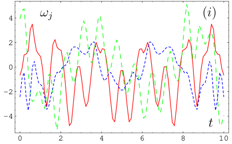
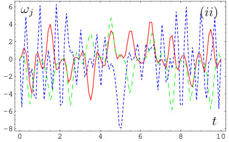
Figure 4: Optimized time dependence of the control parameters of the system Hamiltonian, the solid red, dashed green, and dotted blue line show $\omega_{1,2,3}$, respectively: (i) parameters referring to the graphs (a),(b),(c) in Fig.1; (ii) parameters referring to graphs (d),(e),(f) in Fig.1.

Appendix F Comparison with Uhrig’s DD-sequence

In Figs. 1 and 2 of the main text we compare our results with the following DD sequences:

• a) Concatenated DD (CDD) Khodjasteh and Lidar (2005) defined by

  $$p_{n+1}=p_{n}Xp_{n}Zp_{n}Xp_{n}Z$$ (44)

  with $p_{0}$ $\!=$ $\!f_{\tau}$ denoting free evolution over time $\tau$, where $p^{\mathrm{CDD}}_{1}$ $\!=$ $\!(fXfZ)^{2}$ recovers periodic DD (PDD).

• b) Uhrig-DD (UDD) Uhrig (2007) defined (for $n$ pulses in $Z$) by

  $$p^{\mathrm{UDD}}_{n}=f_{t-\tau_{n}}{Z}f_{\tau_{n}-\tau_{n-1}}{Z}\cdots{Z}f_{\tau_{2}-\tau_{1}}{Z}f_{\tau_{1}}$$ (45)

  with

  $$\tau_{i}=t\sin^{2}[\pi{j}/(2(n+1))],$$ (46)

  where

  $$p^{\mathrm{UDD}}_{1}=fZf$$ (47)

  recovers the spin echo (SE) and

  $$p^{\mathrm{UDD}}_{2}=(fZf)^{2}$$ (48)

  the CPMG-sequence.

• c) Combined CDD and UDD in concatenated UDD (CUDD) Uhrig (2007) defined by concatenating according to

  $$p_{n+1}=p_{n}Xp_{n}X$$ (49)

  an $m$-pulse UDD sequence

  $$p_{0}=p^{\mathrm{UDD}}_{m}$$ (50)

  for $m$ times.

The named basic sequences can be iterated, i.e., repeatedly applied.

Appendix G Leakage from a Subspace

We can adapt our formalism to the situation where the $d$-dimensional state space (to which the relevant quantum information is to be confined) is a subspace of a $N$-dimensional system state space [12]. To do so, the averaging of the initial states $|\Psi\rangle$ is performed on the subspace, for which $|\Psi\rangle$ $\!=$ $\!\hat{P}|\Psi\rangle$, where $\hat{P}$ $\!=$ $\!\sum_{n=1}^{d}|\varphi_{n}\rangle\langle\varphi_{n}|$ is the associated projector. Applying (18) to (B) and defining a matrix $\underline{\bm{\Gamma}}$ $\!=$ $\!\underline{\bm{\Gamma}}^{\dagger}$ with elements

$${\Gamma}_{ik}=\frac{\mathrm{Tr}(\hat{S}_{i}\hat{P}\hat{S}_{k})}{d}-\frac{\mathrm{Tr}(\hat{S}_{i}\hat{P}\hat{S}_{k}\hat{P})+\mathrm{Tr}(\hat{S}_{i}\hat{P})\mathrm{Tr}(\hat{S}_{k}\hat{P})}{d(d+1)},$$ (51)

generalizes (8) to

$$\overline{\langle\Delta\hat{\varrho}(t)\rangle}=\int_{0}^{t}\!\mathrm{d}t_{1}\int_{0}^{t}\!\mathrm{d}t_{2}\mathrm{Tr}\left[\underline{\bm{R}}(t_{1},t_{2})\underline{\bm{\Gamma}}\right],$$ (52)

which recovers (8) for $N$ $\!=$ $\!d$, where ${\Gamma}_{ik}$ $\!=$ $\!\frac{2}{d+1}\delta_{ik}$ $\!=$ $\!2\frac{\kappa}{d}\delta_{ik}$. Equivalently,

$$\overline{\langle\Delta\hat{\varrho}(t)\rangle} = 2\int_{0}^{\infty}\mathrm{d}\omega\,\mathrm{Tr}\bigl{[}\underline{\bm{\epsilon}_{t}}^{\dagger}(\omega)\underline{\bm{G}}_{\mathrm{re}}(\omega)\underline{\bm{\epsilon}_{t}}(\omega)\mathrm{Re}\underline{\bm{\Gamma}}$$ (53)

$$\quad\quad\quad-\underline{\bm{\epsilon}_{t}}^{\dagger}(\omega)\underline{\bm{G}}_{\mathrm{im}}(\omega)\underline{\bm{\epsilon}_{t}}(\omega)\mathrm{Im}\underline{\bm{\Gamma}}\bigr{]}$$

$$= t\,\int_{-\infty}^{\infty}\mathrm{d}\omega\,\mathrm{Tr}[\underline{\bm{G}}_{\mathrm{tot}}(\omega)\underline{\bm{F}_{t}^{\scriptscriptstyle{\Gamma}}}(\omega)],$$

which replaces (9). While $\underline{\bm{G}}_{\mathrm{re}}(\omega)$ $\!=$ $\!\int_{-\infty}^{\infty}\!\mathrm{d}t\;\mathrm{e}^{\mathrm{i}\omega{t}}\;\mathrm{Re}\underline{\bm{\Phi}}(t)$ is identical to $\underline{\bm{G}}(\omega)$ in (9), here we also need $\underline{\bm{G}}_{\mathrm{im}}(\omega)$ $\!=$ $\!\int_{-\infty}^{\infty}\!\mathrm{d}t\;\mathrm{e}^{\mathrm{i}\omega{t}}\;\mathrm{Im}\underline{\bm{\Phi}}(t)$, or the combined $\underline{\bm{G}}_{\mathrm{tot}}(\omega)$ $\!=$ $\!\int_{-\infty}^{\infty}\!\mathrm{d}t\;\mathrm{e}^{\mathrm{i}\omega{t}}\;\underline{\bm{\Phi}}(t)$, whereas in (53) $\underline{\bm{F}_{t}^{\scriptscriptstyle{\Gamma}}}(\omega)$ $\!=$ $\!\frac{1}{t}\underline{\bm{\epsilon}_{t}}(\omega)\underline{\bm{\Gamma}}\underline{\bm{\epsilon}_{t}}^{\dagger}(\omega)$ replaces $\underline{\bm{F}_{t}}(\omega)$ in (9).

(52) encompasses both the internal decoherence effects within the system-subspace associated with $\hat{P}$ and leakage effects related to a population $\overline{\langle\hat{Q}\rangle}$ $\!=$ $\!\overline{\mathrm{Tr}\bigl{[}\hat{\varrho}(t)\hat{Q}\bigr{]}}$ of the orthogonal complement $\hat{Q}$ $\!=$ $\!\hat{I}$ $\!-$ $\!\hat{P}$, averaged over all initial states on $\hat{P}$,

$$\overline{\mathrm{Tr}\bigl{[}\hat{\varrho}(t)\hat{Q}\bigr{]}} = \mathrm{Tr}\bigl{[}\overline{\Delta\hat{\varrho}(t)}\hat{P}\bigr{]}$$ (54)

$$= \int_{0}^{t}\!\mathrm{d}t_{1}\int_{0}^{t}\!\mathrm{d}t_{2}\mathrm{Tr}\left[\underline{\bm{R}}(t_{1},t_{2})\underline{\bm{\Gamma}_{\mathrm{L}}}\right],$$ (55)

$\underline{\bm{\Gamma}_{\mathrm{L}}}$ $\!=$ $\!\underline{\bm{\Gamma}_{\mathrm{L}}}^{\dagger}$ being a matrix with elements

$$({\Gamma}_{\mathrm{L}})_{ik}=\frac{\mathrm{Tr}(\hat{S}_{i}\hat{P}\hat{S}_{k}\hat{Q})}{d}.$$ (56)

If leakage is disregarded in the procedure minimizing $\overline{\langle\Delta\hat{\varrho}(t)\rangle}$, it is likely that a stronger system modulation increases the population of $\hat{Q}$, giving rise to a significant surplus error. This is illustrated in Fig.3, where optimal and PDD-modulations originally designed within a two-level model [as shown in Fig.2(a)] are reconsidered for a two-level subspace of a three-level system. This is done by replacing the Pauli matrices $\hat{\sigma}_{i}$ with the corresponding Gell-Mann matrices $\hat{\gamma}_{i}$, multiplying $\hat{U}(t)$ with $\mathrm{e}^{-\mathrm{i}t{f}\hat{\gamma}_{8}}$ to separate the levels, and adding to $\hat{H}_{\mathrm{I}}$ a leakage term $\hat{\gamma}_{6}\hat{B}_{\mathrm{L}}$. The latter gives rise to an additional bath correlation function $\Phi_{\mathrm{L}}$, assuming here that it can be described by a $1/\omega$-bath coupling spectrum. The total system space is hence spanned by the energy states $|1\rangle$, $|2\rangle$, and $|3\rangle$, the projector onto the relevant subspace is $\hat{P}$ $\!=$ $\!\sum_{n=1}^{2}|{n}\rangle\langle{n}|$, whereas $\hat{Q}$ $\!=$ $\!|3\rangle\langle 3|$, and the states $|\Psi\rangle$ used for averaging are arbitrary superpositions of $|1\rangle$ and $|2\rangle$. The time-independent ${f}$ is a parameter that controls the coupling to the “leakage bath”. It reflects the fact that the energy of the leakage level $|3\rangle$ induces a free evolution, which is shifted to high frequencies for sufficiently large ${f}$, when $|3\rangle$ is strongly energy-detuned from the other two levels, thus providing a “natural” dynamic decoupling of our $1/\omega$-coupling spectrum, and hence the vanishing of the surplus error induced by leakage, justifying the two-level system approximation.

References

• Nielsen and Chuang (2000) M. A. Nielsen and I. L. Chuang, Quantum Computation and Quantum Information (Cambridge University Press, Cambridge, 2000).
• Viola and Lloyd (1998) L. Viola and S. Lloyd, Phys. Rev. A 58, 2733 (1998); D. Vitali and P. Tombesi, Phys. Rev. A 59, 4178 (1999); L. Viola, E. Knill, and S. Lloyd, Phys. Rev. Lett. 82, 2417 (1999); K. Khodjasteh and L. Viola, Phys. Rev. Lett. 102, 080501 (2009).
• Khodjasteh and Lidar (2005) K. Khodjasteh and D. A. Lidar, Phys. Rev. Lett. 95, 180501 (2005); K. Khodjasteh and D. A. Lidar, Phys. Rev. A 75, 062310 (2007).
• Uhrig (2007) G. S. Uhrig, Phys. Rev. Lett. 98, 100504 (2007); G. S. Uhrig, New J. Phys. 10, 83024 (2008); G. S. Uhrig, Phys. Rev. Lett. 102, 120502 (2009); M. J. Biercuk et al., Nature 458, 996 (2009).
• Kofman and Kurizki (2001) A. G. Kofman and G. Kurizki, Phys. Rev. Lett. 87, 270405 (2001); A. G. Kofman and G. Kurizki, Phys. Rev. Lett. 93, 130406 (2004); A. G. Kofman and G. Kurizki, IEEE Trans. Nanotechnology 4, 116 (2005).
• Sagi et al. (2009) Y. Sagi, I. Almog, and N. Davidson (2009), http://arxiv.org/abs/0905.0286; A. Greilich et al., Science 313, 341 (2006a).
• Gordon et al. (2008) G. Gordon, G. Kurizki, and D. A. Lidar, Phys. Rev. Lett. 101, 010403 (2008).
• Gordon et al. (2007) G. Gordon, N. Erez, and G. Kurizki, J. Phys. B: At. Mol. Opt. Phys. 40, S75 (2007).
• Breuer and Petruccione (2002) H.-P. Breuer and F. Petruccione, The Theory of Open Quantum Systems (Oxford University Press, Oxford, 2002).
• Gordon and Kurizki (2006) G. Gordon and G. Kurizki, Phys. Rev. Lett. 97, 110503 (2006).
• Wu et al. (2005) L.-A. Wu, P. Zanardi, and D. A. Lidar, Phys. Rev. Lett. 95, 130501 (2005).
• Wu et al. (2009) L.-A. Wu, G. Kurizki, and P. Brumer, Phys. Rev. Lett. 102, 080405 (2009).
• Agarwal (1996) G. S. Agarwal, Phys. Rev. A 54, R3734 (1996).
• Dankert (2005) C. Dankert, Master’s thesis, University of Waterloo, Ontario, Canada (2005), http://arxiv.org/abs/quant-ph/0512217.