Exploring the Sagittarius Stream
with SEKBO Survey RR Lyrae Stars

Abstract

A sample of RR Lyrae (RRL) variables from the Southern Edgeworth-Kuiper Belt Object survey in regions overlapping the expected position of debris from the interaction of the Sagittarius (Sgr) dwarf galaxy with the Milky Way (RA $\sim$ 20 and 21.5 h; distance = 16–21 kpc) has been followed up spectroscopically and photometrically. The 21 photometrically confirmed type $ab$ RRLs in this region have $\langle$[Fe/H]$\rangle$ = $-1.79\pm 0.08$ on our system, consistent with the abundances found for RRLs in a different portion of the Sgr tidal debris stream. The distribution of velocities in the Galactic standard of rest frame ($V$${}_{\textrm{\scriptsize{GSR}}}$) of the 26 RRLs in the region is not consistent with a smooth halo population. Upon comparison with the Sgr disruption models of Law et al. (2005), a prominent group of five stars having highly negative radial velocities ($V$${}_{\textrm{\scriptsize{GSR}}}$ $\sim-175$ km s^-1) is consistent with predictions for old trailing debris when the Galactic halo potential is modeled as oblate. In contrast, the prolate model does not predict any significant number of Sgr stars at the locations of the observed sample. The observations also require that the recent trailing debris stream has a broader spread perpendicular to the Sgr plane than predicted by the models. We have also investigated the possible association of the Virgo Stellar Stream (VSS) with Sgr debris by comparing radial velocities for RRLs in the region with the same models, finding similarities in the velocity-position trends. As suggested by our earlier work, the stars in the VSS region with large negative $V$${}_{\textrm{\scriptsize{GSR}}}$ values are likely to be old leading Sgr debris, but we find that while old trailing Sgr debris may well make a contribution at positive $V$${}_{\textrm{\scriptsize{GSR}}}$ values, it is unlikely to fully account for the VSS feature. Overall we find that further modeling is needed, as trailing arm data generally favors oblate models while leading arm data favors prolate models, with no single potential fitting all the observed data.

1 Introduction

The notion that the process of galaxy formation involves a protracted, dissipationless merging of protogalactic fragments, consistent with the proposal of Searle & Zinn (1978), is now widely accepted and is consistent with currently favored $\Lambda$ cold dark matter ($\Lambda$CDM) cosmologies. These cosmologies propose that galaxies form via the hierarchical assembly of subgalactic dark halos and the subsequent accretion of cooled baryonic gas (e.g. Springel et al., 2006, and references therein). The outer halo of our galaxy presents an excellent opportunity for probing its formation due to its remoteness and relative quiescence, and has consequently been frequently targeted in searches for relic substructure arising from this accretion process. Bell et al. (2008) gauged quantitatively the relative importance of the accretion mechanism in halo formation by comparing the level of substructure present in Sloan Digital Sky Survey (SDSS) data to simulations, and found that the data are consistent with a halo constructed entirely from disrupted satellite remnants. Starkenburg et al. (2009) reached a similar conclusion from their pencil-beam spectroscopic survey. Systems undergoing disruption in the halo of the Gaxy have indeed been observed, with the most striking example being the Sagittarius (Sgr) dwarf galaxy, located a mere 16 kpc from the Galactic center and showing, through its elongated morphology, unmistakable signs of a strong interaction with the Galaxy (Ibata et al., 1994). The debris from the interaction has subsequently been observed around the sky (Majewski et al., 2003; Newberg et al., 2003; Belokurov et al., 2006), making it arguably the most significant known contributor to the Galactic halo.

Since the discovery of the Sgr dwarf, many studies have reported detections of suspected Sgr tidal debris streams using various tracers including carbon stars from the APM survey (Totten & Irwin, 1998; Ibata et al., 2001), red clump stars from a pencil beam survey (Majewski et al., 1999), RR Lyrae stars from the SDSS (Ivezić et al., 2000; Watkins et al., 2009) and from the Quasar Equatorial Survey Team (QUEST; Vivas et al., 2005), giant stars from the Spaghetti Project Survey (Dohm-Palmer et al., 2001; Starkenburg et al., 2009), A type stars from the SDSS (Newberg et al., 2003) and M giants from the Two Micron All Sky Survey (2MASS; Majewski et al., 2003). Debris associated with Sgr has been found at various angles from the current position of the dwarf, as close as a few kpc from the sun (Kundu et al., 2002) and as far as the distant, outer reaches of the halo (Newberg et al., 2003). Some of the detections were hypothesized to be from older wraps, lost on pericentric passages several Gyr ago (Dohm-Palmer et al., 2001; Kundu et al., 2002; Starkenburg et al., 2009).

Stars stripped from the Sgr dwarf on recent orbits can be unambiguously identified as part of the debris stream via their highly constrained positions and velocities, but the association of older debris can be more difficult and prone to debate. The overdensity in Virgo (Vivas et al., 2001, 2004; Vivas & Zinn, 2006; Newberg et al., 2002; Duffau et al., 2006; Newberg et al., 2007; Jurić et al., 2008; Vivas et al., 2008; Keller et al., 2008; Prior et al., 2009), hereafter referred to by Duffau et al.’s nomenclature as the Virgo Stellar Stream (VSS), is one such example. The VSS has been widely assumed to be a halo substructure which is independent of the Sgr debris, though their association has been hypothesized by Martínez-Delgado et al. (2007) who showed that Law et al.’s (2005) model of the Sgr leading tidal tail passes through the region of the VSS. However, the model predicts highly negative radial velocities in the Galactic standard of rest (GSR) frame for Sgr stars in this region, contrary to observations of a peak velocity at V${}_{\textrm{\scriptsize{GSR}}}\sim 100$–$130$ km s^-1 (Duffau et al., 2006; Newberg et al., 2007; Prior et al., 2009). A possibility which has received little attention thus far is the association of the VSS with the trailing Sgr debris stream, whose members are indeed predicted to have positive velocities in this region. Martínez-Delgado et al., commenting that in certain models both leading and trailing arms overlap the VSS region, noted this possibility only in passing. On the other hand, the models predict a relatively low density of Sgr debris in this region which is at odds with the significance of the observed overdensity. Newberg et al. (2007) also note that the VSS is not spatially coincident with the main part of the Sgr leading tidal tail, but that the features do significantly overlap. It is thus clear that no consensus has yet been reached regarding the association of the VSS with the Sgr Stream. The current study addresses this question in §3 with intriguing results (see also Starkenburg et al., 2009).

As alluded to above, the wealth of observational data for potential Sgr Stream members has motivated several attempts at modeling the disruption of the Sgr dwarf and predicting the positions and radial velocities of the ensuing debris particles (e.g. Johnston et al., 1999; Ibata et al., 2001; Helmi & White, 2001; Martínez-Delgado et al., 2004; Law et al., 2005; Fellhauer et al., 2006). These models have resulted in estimates of the orbit pericenter and apocenter, Sgr’s transverse velocity and current bound mass. In addition, several studies, considering the debris as test particles, have drawn conclusions about the shape of the Galactic halo potential. For example, from the observation that the Sgr stream identified in their carbon star sample traces a great circle, Ibata et al. (2001) concluded that the halo must be almost spherical. Moreover, on the basis of N-body simulations, they subsequently constrained the mass distribution in the dark halo and concluded that it too was most likely spherical. However, Helmi (2004a) asserted that debris lost recently, such as M giant data in the trailing arm, is too young dynamically to provide any constraints on the shape of the dark halo potential. Nevertheless debris lost at earlier times can discriminate between prolate (flattening $q>1$), spherical ($q=1$) and oblate ($q<1$) shapes for the potential (Helmi, 2004a).

The issue of dark halo shape remains clouded, however, since a range of contrasting views have also been presented in recent years. Helmi (2004b) found that results from M giants in the leading arm supported a notably prolate halo ($q=1.7$). On the other hand, Martínez-Delgado et al. (2004), using the various reported distances and radial velocities available in the literature, obtained an oblate halo ($q=0.85$) in their simulations. Based on RR Lyrae stars located in the leading arm at a distance of $\sim$50 kpc, Vivas et al. (2005) found that the models of Martínez-Delgado et al. (2004) and Helmi (2004a) with spherical or prolate halos fit the data better than those for an oblate halo. Law et al. (2005) performed the first simulations based on the 2MASS all-sky view of the Sgr debris streams. They noted that the velocities of leading debris were better fit by prolate halos, whereas trailing debris velocity data had a slight preference for oblate halos. Confusing the matter, however, was the observation that the orbital pole precession of young debris favors oblate models. Fellhauer et al. (2006) found that only halos close to spherical resulted in bifurcated streams, such as that evident in Belokurov et al.’s (2006) analysis of upper main sequence and turn off stars in SDSS data. Finally Starkenburg et al. (2009) favor spherical or prolate halo shapes when comparing the Sgr debris in their pencil-beam survey with the models of Helmi (2004a).

The brief discussion above illustrates that the shape of the dark halo is a point of contention, with no model being capable of fitting all the available data. Law et al. (2005) propose that evolution of the orbital parameters of Sgr over several Gyr is needed to explain the results and suggest dynamical friction as the most likely mechanism to bring this about. They note that this would require Sgr to have been an order of magnitude more massive 2 Gyr ago. They also recognize the need to model the dwarf as a two-component system, with the dark matter bound less tightly than the baryons and indicate that such a study is underway. Inclusion of additional, newly discovered samples of observed Sgr stream stars will no doubt help to more tightly constrain these improved models, particularly samples containing old stars which potentially were lost several pericentric passages ago and which have been influenced by the Galactic halo potential for a longer time period.

Being Population II stars, RR Lyrae (RRL) variable stars are an excellent choice of tracer for unraveling the history of the Sgr-Milky Way interaction and for further elucidating the shape of the dark halo. We have undertaken a project using RRLs which encompasses these aims, while more generally seeking to gain further insight into the role of accretion in galaxy formation. Although our broad goal was to identify and characterize substructures in the Galaxy’s halo, ultimately the project transpired to focus on two such substructures in detail: the Virgo Stellar Stream and the Sagittarius Stream. A companion paper (Prior et al., 2009, hereafter Paper I) describes in detail the entire set of observations, along with results and analysis for the VSS region. In the current paper, results for our RRL samples in the Sgr region are presented. Specifically, after giving a brief overview of the observations in §2, radial velocities for RRLs in the Sgr region are presented in §3, and comparisons are made to Law et al.’s (2005) recent N-body simulations of the disruption of the Sgr dwarf, which adopt various modeled shapes for the dark halo potential. At this point, data from the VSS region are also included in order to explore their possible association with Sgr debris. §4 then presents metallicities of the Sgr region RRLs. The paper ends with a general discussion and conclusions.

2 Observations

The reader is referred to Paper I for a detailed account of target selection, observations and data reduction. Key points are reiterated below. The radial distribution of RRL candidates obtained by Keller et al. (2008, hereafter KMP08) from the Southern Edgeworth-Kuiper Belt Object (SEKBO) survey data revealed several overdensities compared to simulated smooth halos. The two main overdensities selected for follow-up spatially coincided with the VSS (observed sample: 8 RRLs at RA $\sim$ 12.4 h and 3 RRLs at RA $\sim$ 14 h; Paper I), and a portion of the Sgr debris stream (observed sample: 5 RRLs at RA $\sim$ 20 h and 21 RRLs at RA $\sim$ 21.5 h; this paper). The stars in both samples have extinction corrected magnitudes $V_{0}\sim 17$. Although the possible association of the VSS with Sgr debris is investigated here, for ease of reference and for consistency with Paper I, we refer to the samples of RRLs at $\sim$12.4 h and $\sim$14 h as being in the “VSS region” and to the samples at $\sim$20 h and $\sim$21.5 h as being in the “Sgr region”.

In particular, we show in Fig. 1 the number density of SEKBO RRL candidates as a function of heliocentric distance for the Right Ascension range 21.0 h $\leq$ RA $\leq$ 22.0 h. There is a clear excess at distance of $\sim$20 kpc above the number density predicted for a smooth halo distribution, which KMP08 ascribe to Sgr debris. The “Sgr region” RRLs observed here have a mean distance of 19.1 kpc with a range of 16 to 21 kpc, and clearly probe this density excess.

Figure 1: The number density distribution of SEKBO RRL candidates for the RA range 21 h – 22 h as a function of heliocentric distance. The open circles are the individual data points and the filled circles are the stars observed in the 21.5 h region. The solid lines are the smooth halo density distribution derived from the entire SEKBO sample (see Keller et al. (2008) for details). The marked excess at $\sim$20 kpc is due to Sgr.

As discussed in Paper I, photometric and spectroscopic observations were made at Siding Spring Observatory in six six-night runs between November 2006 and October 2007, with the Australian National University $40^{\prime\prime}$ and 2.3 m telescopes, respectively. For photometry, 5–19 (average 9) observations per star enabled confirmation of the RR Lyrae classifications through period and light curve fitting in addition to providing ephemerides. For spectroscopy, 1–4 observations were taken for each target using the blue arm of the Double Beam Spectrograph. Spectra were centred on $4350$ Å and have a signal-to-noise of $\sim$20 and a resolution of $\sim$2 Å. The photometric and spectroscopic data reduction procedures are described in Paper I and a photometric data summary, including positions, magnitudes, periods and amplitudes of all targets, is provided in Table 2 of that paper.

3 Radial Velocities

The general method of obtaining radial velocities consisted of cross correlating each wavelength-calibrated target spectrum with several template spectra (radial velocity standard stars, for example). For each type $ab$ RRL, the velocities corresponding to different epochs were then phased using ephemerides from the photometric data, and a systemic velocity was subsequently assigned by fitting a template RRL velocity curve (characterizing the RR$ab$ variation of velocity with phase). The average velocity was used as the systemic velocity for type $c$ RRLs. Finally, the heliocentric systemic velocity was converted to a velocity in the Galactic standard of rest frame. The uncertainty in the $V$${}_{\textrm{\scriptsize{GSR}}}$ values is $\pm 20$ km s^-1. Full details of the method are given in Paper I.

Table 1 summarizes results from the spectroscopic data for the 26 RRLs in the Sgr region, including the systemic $V$${}_{\textrm{\scriptsize{GSR}}}$ values. Results for the VSS region stars are also included for ease of reference; see following discussion. The distributions of $V$${}_{\textrm{\scriptsize{GSR}}}$ values in the 20 h (5 stars) and in the 21.5 h (21 stars) Sgr regions are presented as generalized histograms in Fig. 2 (note that results from the two regions are not combined since the pattern of radial velocities of Sgr Stream stars varies with position, as discussed further below). Shown also in the figure are the expected distributions for a halo RRL velocity distribution that has $\langle$$V$${}_{\textrm{\scriptsize{GSR}}}$$\rangle$ = 0 km s^-1 and $\sigma$ = 100 km s^-1(e.g., Sirko et al., 2004; Brown et al., 2005). This “smooth halo” velocity distribution is normalised with the assumption that the observed samples are entirely drawn from such a halo population though Fig. 1 suggests this is not likely to be the case. In the 20 h region, there is an apparent excess of stars having highly positive radial velocities ($V$${}_{\textrm{\scriptsize{GSR}}}$ $\approx 200$ km s^-1), while in the 21.5 h region an excess (five stars) is evident at highly negative velocities ($V$${}_{\textrm{\scriptsize{GSR}}}$ $\approx-175$ km s^-1). There is also an apparent lack of stars with $-125<$ $V$${}_{\textrm{\scriptsize{GSR}}}$ $<-50$ km s^-1.

To investigate the statistical significance of these features we have conducted Monte-Carlo simulations in which samples of size equal to the observed samples were drawn randomly from the assumed smooth halo velocity distribution, and convolved with a 20 km s^-1 kernel as for the observations. The results are also displayed in Fig. 2 where the upper and lower contours that enclose 95% of the trials are shown by the dotted lines. These simulations show that in the 20 h region, the excess at $V$${}_{\textrm{\scriptsize{GSR}}}$ $\approx 200$ km s^-1 is indeed significant, as is the excess at $V$${}_{\textrm{\scriptsize{GSR}}}$ $\approx-175$ km s^-1 in the 21.5 h region, even with the assumption that the samples are entirely drawn from the smooth halo distribution. In conjunction with the results of Fig. 1 in which there is a clear excess above the smooth halo model, the results suggest strongly that both samples contain velocity components that are not simply random selections from a smooth halo. The apparent deficiency of stars centered at $V$${}_{\textrm{\scriptsize{GSR}}}$ $\approx$ –75 km s^-1 in the 21.5 h sample also appears to be statistically significant.

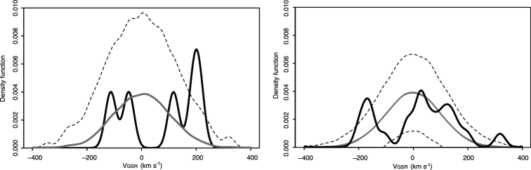
Figure 2: Generalized histograms of $V$${}_{\textrm{\scriptsize{GSR}}}$ (with kernel of 20 km s^-1) for observed RRLs in the Sgr region. Left: the 5 RRLs in the 20 h region; Right: the 21 RRLs in the 21.5 h region. Overplotted in each panel as a solid gray line is the expected distribution of $V$${}_{\textrm{\scriptsize{GSR}}}$ for a halo population of the same size as the observed samples in which velocities are normally distributed with $\langle$$V$${}_{\textrm{\scriptsize{GSR}}}$$\rangle$ = 0 km s^-1 and $\sigma$ = 100 km s^-1. The 95% confidence intervals for samples drawn from this distribution are shown by the dashed lines. In the 20 h region, there is a statistically significant excess of stars with highly positive velocities ($V$${}_{\textrm{\scriptsize{GSR}}}$ $\sim 200$ km s^-1) while in the 21.5 h region, there is a similar statistically significant excess of stars with highly negative velocities ($V$${}_{\textrm{\scriptsize{GSR}}}$ $\sim-175$ km s^-1).

Table 1: Spectroscopic data summary

ID	$\Lambda_{\odot}$	$B_{\odot}$	RRL	systemic vel.	n${}_{\textrm{\scriptsize{vel}}}$	$V$${}_{\textrm{\scriptsize{helio}}}$	$V$${}_{\textrm{\scriptsize{GSR}}}$	n${}_{\textrm{\scriptsize{Fe/H}}}$	[Fe/H]
	(deg)	(deg)	type	calculation		(km s-1)	(km s-1)
—–Sgr region—–
109582-3724	$10.6$	$-10.5$	$ab$	fit	3	$129$	$211$	4	$-1.93$
109464-5627	$10.9$	$-10.2$	$ab$	average	4	$36$	$117$	-	-
109489-3076	$10.9$	$-10.4$	$ab$	fit	3	$-129$	$-47$	3	$-1.85$
109489-2379	$11.1$	$-10.2$	$ab$	fit	3	$108$	$191$	3	$-2.17$
109463-3964	$11.5$	$-10.8$	$ab$	fit	2	$-197$	$-113$	3	$-1.58$
125857-20	$27.1$	$-16.2$	$ab$	fit	1	$-1$	$109$	1	$-2.00$
110828-1100	$29.3$	$-10.7$	$ab$	fit	3	$-250$	$-159$	3	$-1.76$
126040-78	$29.5$	$-8.9$	$ab$	fit	2	$-50$	$34$	2	$-1.45$
110823-641	$29.7$	$-10.9$	$c$	average	3	$-112$	$-20$	-	-
114793-1530	$30.2$	$-16.1$	$c$	average	3	$51$	$162$	-	-
126093-1135	$30.3$	$-8.0$	$ab$	fit	3	$56$	$137$	3	$-1.53$
126536-714	$31.0$	$-7.2$	$ab$	fit	1	$55$	$134$	3	$-0.73$
99747-73	$31.6$	$-11.9$	$ab$	fit	1	$-77$	$20$	3	$-2.55$
102297-1488	$32.3$	$-13.6$	$ab$	fit	3	$-290$	$-187$	4	$-1.53$
110735-595	$32.5$	$-15.2$	$ab$	average	4	$-277$	$-169$	4	$-1.62$
102292-1096	$33.4$	$-14.4$	$ab$	fit	2	$92$	$198$	2	$-1.61$
126245-763	$33.7$	$-8.7$	$ab$	fit	1	$-13$	$72$	1	$-1.56$
102601-1489	$35.1$	$-13.0$	$ab$	fit	2	$-123$	$-22$	3	$-2.26$
102601-400	$35.3$	$-12.8$	$ab$	fit	2	$-301$	$-201$	3	$-1.98$
110753-346	$35.7$	$-12.3$	$ab$	fit	2	$221$	$319$	3	$-2.00$
110827-579	$36.5$	$-11.5$	$ab$	fit	3	$-252$	$-157$	2	$-1.51$
99752-96	$36.5$	$-12.7$	$c$	average	3	$-74$	$26$	-	-
110738-411	$37.2$	$-12.0$	$ab$	fit	4	$-206$	$-107$	4	$-2.10$
113345-1032	$37.6$	$-11.5$	$c$	average	3	$7$	$103$	-	-
115381-767	$38.8$	$-12.5$	$ab$	fit	2	$-74$	$26$	3	$-2.01$
115381-349	$39.4$	$-12.6$	$ab$	fit	1	$-38$	$63$	2	$-1.87$
—–VSS region—–
108227-529	$262.5$	$17.8$	$c$	average	1	$-8$	$-119$	-	-
96102-170	$263.7$	$15.2$	$ab$	fit	2	$230$	$128$	3	$-2.15$
120185-77	$264.7$	$13.0$	$ab$	fit	2	$94$	$1$	2	$-2.38$
107552-323	$268.2$	$18.0$	$ab$	fit	3	$302$	$193$	3	$-1.34$
119827-670	$269.0$	$17.7$	$ab$	fit	2	$-84$	$-192$	2	$-1.68$
120679-336	$269.8$	$19.5$	$ab$	fit	3	$204$	$91$	2	$-1.74$
121194-205	$273.4$	$20.0$	$c$	average	1	$-39$	$-152$	-	-
121242-188	$274.3$	$22.4$	$c$	average	3	$276$	$155$	-	-
120698-392	$285.9$	$16.8$	$c$	average	1	$227$	$134$	-	-
109247-528	$286.4$	$14.7$	$c$	average	2	$113$	$28$	-	-
105648-222	$287.0$	$11.2$	$ab$	fit	1	$-91$	$-162$	1	$-1.45$

In order to further investigate the pattern of radial velocities and to explore how well they agree with expectations for Sgr Stream stars, we have compared the velocities to those predicted by the recent models of Law et al. (2005) (hereafter LJM05). While a number of other models for the disruption from the Sgr-Milky Way interaction exist (see §1 for a brief review), LJM05’s models were chosen for the comparison as they are currently the only models based on a complete all-sky view of the tidal streams of Sgr (namely, the 2MASS M giant sample). They use N-body simulations to predict the heliocentric distances and radial velocities of $10^{5}$ particles stripped from the Sgr dwarf up to four orbits ago (i.e. up to approximately 3 Gyr ago). Three models of the flattening, $q$, of the Galactic dark halo potential are considered: prolate ($q$ = 1.25), spherical ($q$ = 1.0) and oblate ($q$ = 0.90). Their simulations adopt a spherical, Sun-centered, Sgr coordinate system, with the longitudinal coordinate, $\Lambda_{\odot}$, being zero in the direction of the Sgr core and increasing along the Sgr trailing debris stream. The zero plane of the latitude coordinate, $B_{\odot}$, is defined by the best fit great circle of the Sgr debris. For the purpose of clarifying the discussion which follows, Fig. 3 shows $V$${}_{\textrm{\scriptsize{GSR}}}$ plotted against $\Lambda_{\odot}$ for the case of the prolate potential (selected due to its more easily identifiable streams compared to oblate and spherical potentials). All $B_{\odot}$ values are shown. The Sgr core is, by definition, located at $\Lambda_{\odot}$ = 0^∘, the leading stream is highlighted by the green dashed line and the trailing stream by the blue dotted line. In addition, certain parts of the streams have been labeled (a–d) for future reference. In the text which follows, they are referred to as, for example, “debris-c”, where the $\Lambda_{\odot}$ range should also be taken into account in order to focus on the relevant stream section.

Figure 3: Radial velocities against $\Lambda_{\odot}$ from Law et al.’s (2005) model with a prolate Galactic halo potential. Particles at all distances are shown (see Figs 4 and 5 for distance-coding). By definition, the Sgr dwarf is located at $\Lambda_{\odot}$ = 0^∘. The leading arm is highlighted by the green dashed line and the trailing arm by the blue dotted line. For ease of reference, certain parts of the stream have been identified: (a) new trailing debris (current perigalactic passage); (b) very old trailing debris (4 orbits ago); (c) old leading debris (3–4 orbits ago); and (d) very old leading debris (4 orbits ago). All $B_{\odot}$ values are shown.

Figure 4 shows the distribution of $V$${}_{\textrm{\scriptsize{GSR}}}$ as a function of $\Lambda_{\odot}$ for LJM05’s simulated particles assuming prolate, spherical and oblate halo potentials. All $B_{\odot}$ values are shown. Our observed RRLs are at heliocentric distances 16–21 kpc. The distances are based on the assumption of $M_{V}$ = 0.56 and have an uncertainty of $\sim$7%, as described in KMP08. This corresponds to an uncertainty of approximately $\pm$1 kpc at a distance of 20 kpc. In order to isolate simulated stars at similar distances to the observed stars, the plot is color-coded, with red dots representing particles at 6–31 kpc (i.e. 10 kpc closer/farther than our observed range). All other distances are color-coded gray. The choice to consider a wider distance range for the simulated particles than for our observational data was motivated by the significant uncertainties involved in the modeled distances. The major factor contributing to this is the 17% distance uncertainty for 2MASS M giant stars, stemming from the uncertainty in the values of the solar distance from the Galactic center and from Sgr. LJM05 note that the estimated size of Sgr’s orbit scales according to the M giant distance scale, and distances to simulated debris particles similarly. However, of course an orbit cannot be scaled up or down in distance without affecting the velocities, and thus the distance uncertainty necessarily implies an equivalent velocity uncertainty.

We also show, for comparison, equivalent plots highlighting simulated particles at the observed distances of 16–21 kpc in Fig. 5. Again all $B_{\odot}$ values are included. Overplotted on Figs 4 and 5 as filled circles are our observational data in the Sgr region, with the 20 h region corresponding to $\Lambda_{\odot}$ $\approx$ 10^∘ and the 21.5 h region corresponding to $\Lambda_{\odot}$ $\approx$ 25–40^∘. In order to explore their possible association with the Sgr Stream (as discussed in §1), our observed RRLs in the VSS region are also plotted (triangles at $\Lambda_{\odot}$ $\approx$ 260–290^∘).

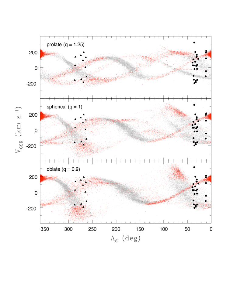
Figure 4: Radial velocities against $\Lambda_{\odot}$ from models with prolate (top), spherical (middle) and oblate (bottom) Galactic halo potentials (Law et al., 2005). Red dots denote simulated stars with heliocentric distances $d$ = 6–31 kpc while gray denotes stars at all other distances. Overplotted are values for the 26 observed RRLs in the 20 h and 21.5 h Sgr regions (circles) and the 11 RRLs in the VSS region (triangles). Note that, at the relevant distance, only the oblate model is able to predict the group of stars at $\Lambda_{\odot}$ $\approx$ 35^∘ which are observed to have highly negative $V$${}_{\textrm{\scriptsize{GSR}}}$. All $B_{\odot}$ values are shown.

Figure 5: Radial velocities against $\Lambda_{\odot}$ from models with prolate (top), spherical (middle) and oblate (bottom) Galactic halo potentials (Law et al., 2005). Red dots denote simulated stars with heliocentric distances $d$ = 16–21 kpc while gray denotes stars at all other distances. Overplotted are values for the 26 observed RRLs in the 20 h and 21.5 h Sgr regions (circles) and the 11 RRLs in the VSS region (triangles). All $B_{\odot}$ values are shown.

In both Figs 4 and 5 the model particles are plotted for all values of the latitude coordinate $B_{\odot}$. However, it is necessary to keep in mind that the RRLs observed here are drawn from the SEKBO survey, which has the ecliptic as its mid-plane, not the Sgr orbit plane. Thus, the SEKBO RRLs do not sample all the $B_{\odot}$ values at any given $\Lambda_{\odot}$. For example, the RRLs in the 20 h and 21.5 h regions have –16.2 $\leq$ $B_{\odot}$ $\leq$ –7.2 while those in the VSS region have 11.2 $\leq$ $B_{\odot}$ $\leq$ 22.4 (cf. Table 1). Specifically, as discussed in KMP08, the SEKBO survey plane cuts through the Sgr plane at an angle of $\sim$16$\arcdeg$ with an opening angle of 10$\arcdeg$. Consequently, we show in Figs 6 and 7 the same data as for Figs 4 and 5, but now with the model particles plotted only if they fall within a $\pm$5$\arcdeg$ window about the SEKBO survey mid-plane. Nevertheless, given that the definition of the $B_{\odot}$ = 0 plane is model dependent, where appropriate we will continue to show figures with both the full $B_{\odot}$ range and with the restricted range required by the SEKBO survey characteristics.

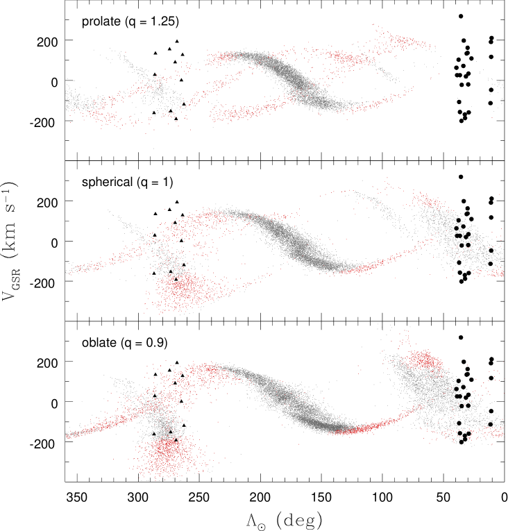
Figure 6: As for Fig. 4, i.e. model particle distances from 6–31 kpc, except that the model points plotted have $B_{\odot}$ values that fall within the SEKBO survey region.

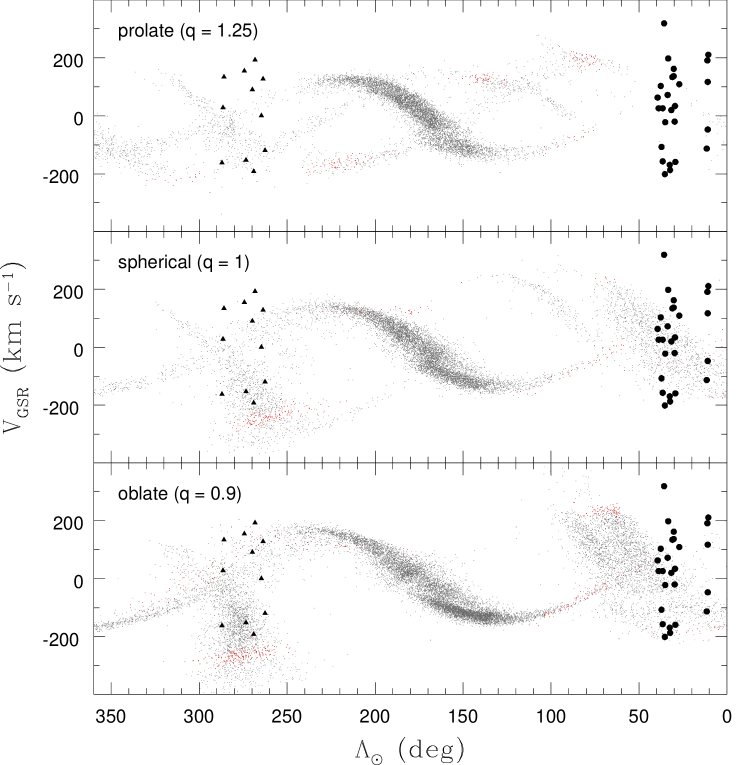
Figure 7: As for Fig. 5, i.e. model particle distances from 16–21 kpc, except that the model points plotted have $B_{\odot}$ values that fall within the SEKBO survey region.

3.1 20 and 21.5 h Sgr regions

A comparison between the observed and simulated data in the 20 and 21.5 h regions reveals several points of interest. Considering first the location of the five 20 h stars in Fig. 4, it is tempting to associate the 3 stars with large positive $V$${}_{\textrm{\scriptsize{GSR}}}$ values with the recent trailing debris of the models, the location of which is largely independent of the halo potential adopted. However, inspection of Fig. 6 indicates that such an interpretation is not clear-cut: the recent trailing debris in the models lies relatively close to the $B_{\odot}$ = 0 plane and thus the number of model points from this feature is significantly reduced when the restriction to the SEKBO survey region is applied, and for the case of the prolate halo model, it is questionable as to whether the observed stars are related to Sgr at all. These conclusions are not substantially altered with the more restricted in distance views shown in Figs 5 and 7. We also note that the distance to Sgr itself is $\sim$28 kpc (e.g. Sarajedini & Layden, 1995) so that the number of model points in the vicinity of $\Lambda_{\odot}$ = 0 in Figs 5 and 7 is naturally reduced compared to the figures with the wider distance range.

The larger number of stars in the 21.5 h sample, however, provides a stronger basis on which to make comparisons with the model predictions. Adopting the underlying smooth halo density distribution from Fig. 1, we expect that the 21.5 h sample has a field halo contamination of $\sim$40%, or 8 $\pm$ 3 stars; the remainder are likely to be associated with Sgr. In both Figs 4 and 5 there is a group of seven stars centered at $\Lambda_{\odot}$ $\approx$ 35^° and $V$${}_{\textrm{\scriptsize{GSR}}}$ $\approx$ 100 km s^-1 whose variation of $V$${}_{\textrm{\scriptsize{GSR}}}$ with $\Lambda_{\odot}$ suggests that they are members of the recent trailing debris stream (debris-a) regardless of the halo potential adopted. There are also, however, of order six stars with –25 $\leq$ $V$${}_{\textrm{\scriptsize{GSR}}}$ $\leq$ 40 km s^-1 which show no obvious connection to any stream in any model. Presumably a substantial fraction of these are field halo objects, as is most likely the highest velocity star in the sample. There is then an apparent gap with no stars found between $V$${}_{\textrm{\scriptsize{GSR}}}$ $\approx$ –25 and $V$${}_{\textrm{\scriptsize{GSR}}}$ $\approx$ –110 km s^-1. We suggested above that this gap may be statistically significant, and based on the simulated particles it could plausibly be interpreted as dividing members of the old leading debris stream (debris-c) from the old trailing stream (debris-b). The most notable feature, however, is the group of five stars with highly negative radial velocities ($\langle$$V$${}_{\textrm{\scriptsize{GSR}}}$$\rangle$= $-175$ km s^-1, $\sigma$ = 19 km s^-1, slightly less than the uncertainty in the measurements) which we noted as a distinct peak in Fig. 2. Under the smooth halo velocity distribution assumption stated above, we would expect a negligible number (0.4 $\pm$ 0.1) of the expected 5–11 contaminating halo field RRLs in the 21.5 h sample to have $V$${}_{\textrm{\scriptsize{GSR}}}$ values between –200 and –150 km s^-1. The significance of the feature is thus beyond question. Comparing this observed group of RRLs with the simulated particles in Figs 4 and 5, it is clear that only the oblate model predicts any significant number of stars with such velocities at the appropriate distances. In fact, the association of this group of stars with Sgr debris arguably rules out the prolate model for the halo potential, at least in the context of the Law et al. (2005) models.

Once again, however, these possible interpretations need to be weighed when the observations and the models are considered in the context of the SEKBO survey selection window (Figs 6 and 7). Identification of any of the observed stars with Sgr then becomes problematical in the case of the prolate halo potential, as was noted above for the 20 h sample. Also as was noted for the 20 h sample, the models of LJM05 do not predict any recent trailing debris at the $B_{\odot}$ values of the 21.5 h sample stars regardless of the adopted halo potential. Significantly, however, as seen in the bottom panel of Fig. 6, the LJM05 model with the oblate halo potential continues to predict the existence of a population of stars with large negative $V$${}_{\textrm{\scriptsize{GSR}}}$ values at $\Lambda_{\odot}$ values similar to those of the 21.5 hr sample, even when the model points are limited to the SEKBO survey region. This remains the case when the model points are more restricted in distance, as shown in Fig. 7. Indeed, in the context of the Law et al. (2005) models, the identification of this group of stars as Sgr debris strongly supports an oblate model for the halo potential.

To investigate the reliability of the qualitative interpretations presented above, we have conducted a number of Monte-Carlo trials. In these trials we have chosen individual $V$${}_{\textrm{\scriptsize{GSR}}}$ values randomly from the set of model particle velocities, subject to: (1) the SEKBO selection window; (2) the $\Lambda_{\odot}$ range of the 21.5 h observed sample; and (3) distance limits of 6-31 kpc (cf. Fig. 6). We have also selected randomly from the assumed smooth halo velocity distribution, with the “Sgr” and “field halo” selections in the ratio 0.6 to 0.4. The total selected sample for each trial is set equal to that for the observed 21.5 h sample (i.e. 21 stars). The velocities are then convolved with the observed $V$${}_{\textrm{\scriptsize{GSR}}}$ errors of 20 km s^-1 and a generalized histogram constructed. Multiple trials then allow the generation of a mean generalized histogram and $\pm$3$\sigma$ limits about that mean as a function of $V$${}_{\textrm{\scriptsize{GSR}}}$. We can then investigate the extent to which the observed velocity distribution (cf. Fig. 2) is consistent with the “model + field halo” predictions. The results are shown in Fig. 8 for the LJM05 models with spherical and oblate potentials. We cannot perform this test for the prolate models as there are simply insufficient model points meeting the criteria to allow adequate sampling. Similarly, there are also insufficient model points to carry out the simulations with the distances restricted to 16–21 kpc.

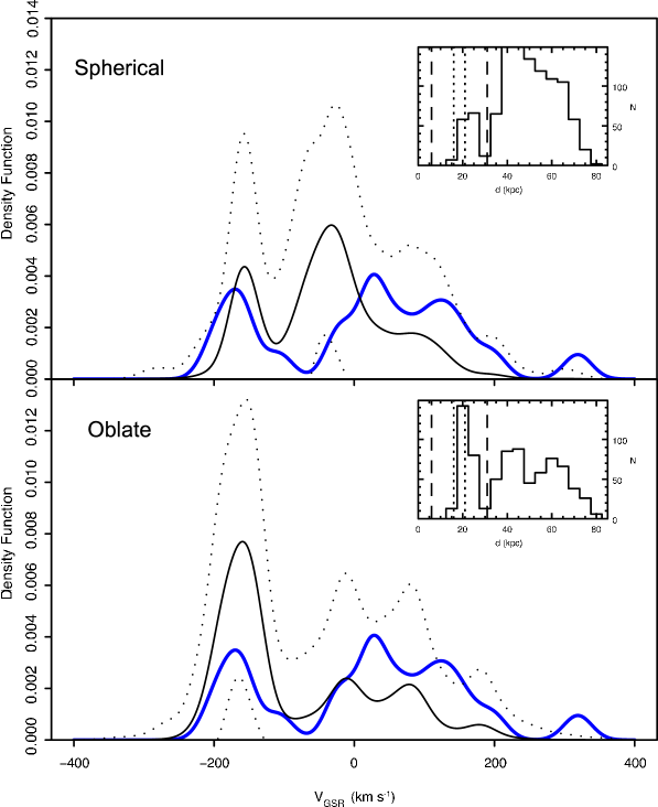
Figure 8: Comparison of the generalised histogram for the observed $V$${}_{\textrm{\scriptsize{GSR}}}$ velocities of the 21.5 h sample (blue solid line, cf. right panel of Fig. 2) with predictions from the LJM05 models. The upper panel is for the spherical halo potential model and the lower panel is for the oblate model. In each panel the black solid line is the mean generalized histogram from the “model + field halo” trials (see text for details), while the dotted lines are the $\pm$3$\sigma$ bounds from the trials. For both models the observed distribution lies within the trial boundaries. The inset histograms show the distance distribution of simulated stars for each halo potential in the $\Lambda_{\odot}$ and $B_{\odot}$ range appropriate for the observed sample. Note that Law et al. (2005) added a 17% artificial random distance scatter to the simulated particles to mimic the photometric distance error in the 2MASS sample. The vertical dashed lines indicate the distance range of the model particles used in the trials (6–31 kpc), while the vertical dotted lines indicate the distance range of the observed stars (16–21 kpc).

It is nevertheless apparent from Fig. 8 that the observed data are largely consistent with the “model + field halo” predictions for both the spherical and oblate halo potential models. For the spherical model, the largest difference between the observations and the model predictions lies at $V$${}_{\textrm{\scriptsize{GSR}}}$ values of approximately –50 km s^-1, where the model predicts a peak in the velocity distribution while the observations show a deficiency. The discrepancy marginally exceeds the 3$\sigma$ bound but we do not regard it as strong enough to definitely rule out the spherical halo model. In the oblate case, the biggest difference is that the model predicts a larger number of stars at large negative $V$${}_{\textrm{\scriptsize{GSR}}}$ than are actually observed, although the data are within the $3\sigma$ bound and there is close agreement as regards the location of the velocity peak. Further, as distinct from the spherical case, for the oblate model there is agreement with the observations as regards the deficiency of stars around $V$${}_{\textrm{\scriptsize{GSR}}}$ $\approx$ –50 km s^-1. As noted above, it is tempting to identify this gap as separating the old leading debris stream (debris-c) from the old trailing stream (debris-b).

At this point it is also useful to consider the distance distribution of the simulated particles in the different models. The inset distance histogram in Fig. 8 shows that for the oblate model and the relevant $\Lambda_{\odot}$ and $B_{\odot}$ range, the density of the model particles peaks around 20 kpc and then falls off as the distance approaches 30 kpc, with a second peak at distances $\sim$40 kpc. The location of this peak in the model distribution is consistent with the peak in the observed density distribution of the SEKBO RRLs seen at this distance in Fig. 1. The spherical model, however, shows a less marked peak at $\sim$25 kpc with the majority of the model particles lying at $\sim$40 kpc and beyond.

In summary, the stars of the 21.5 h sample are most consistent with the predictions of the oblate halo potential model of LJM05. In contrast, the prolate model does not predict any significant number of Sgr debris stars at the $\Lambda_{\odot}$ and $B_{\odot}$ values of the observed sample, and at the very least, requires modification if it is to be viable. The spherical potential model is not inconsistent with the observations, but predicts stars with velocities where the observations show a definite lack. In all cases, however, the observations seem to require that the recent trailing debris stream has a larger spread in $B_{\odot}$ than predicted by any of the models.

3.2 12.4 and 14 h VSS regions

Thus far we have only discussed RRLs in the 20 and 21.5 h Sgr regions. We now turn our attention to the RRLs in the VSS region. We note first that the SEKBO survey data (Keller et al., 2008) indicates a significant overdensity at the distance and direction of these RRLs, so the degree of contamination from field halo RRLs is likely to be small. The VSS RRLs from Paper I are divisible into two groups: four stars with significant negative $V$${}_{\textrm{\scriptsize{GSR}}}$ values, and 7 stars with $V$${}_{\textrm{\scriptsize{GSR}}}$ values that range from near zero to $\sim$200 km s^-1. For both groups it appears that the velocities are somewhat higher for lower $\Lambda_{\odot}$ values.

To explore the potential association of these stars with Sgr debris streams we once again consider their location in the context of the LJM05 models: Figs 4 and 5 show the model data for all $B_{\odot}$ values while Figs 6 and 7 show the model data restricted to SEKBO survey range. The VSS region RRLs are the 11 stars with $\Lambda_{\odot}$ $\approx$ 260–290^∘.

Turning first to the prolate case in Figs 4 and 6, we see that the 4 stars with significant negative $V$${}_{\textrm{\scriptsize{GSR}}}$ velocities lie in the region of model particles from old leading debris (debris-d) (cf. Paper I) and the velocity trend with $\Lambda_{\odot}$ is consistent with that of the models. This remains the case when the model $B_{\odot}$ values are restricted to the SEKBO survey region. Are these stars, which have $\langle$$V$${}_{\textrm{\scriptsize{GSR}}}$$\rangle$ = –156 km s^-1, part of a real Sgr related substructure? In this region, Newberg et al. (2007) detected a group of F stars in SDSS data having a similar velocity ($V$${}_{\textrm{\scriptsize{GSR}}}$ $\approx$ –168 km s^-1). More recently, in QUEST data, Vivas et al. (2008) found a significant number of Blue Horizontal Branch stars at a similar velocity ($V$${}_{\textrm{\scriptsize{GSR}}}$ $\approx$ –171 km s^-1) as well as two RRLs. They place the group at 11 $\pm$ 2 kpc, but note that the stars are near the faint limit of their sample and suggest that it may be the near side of a larger substructure. They believe it to be the same feature as that identified by Newberg et al., which has a quoted distance of 11–14 kpc. Vivas et al. note that the nominal 16% distance uncertainty in Newberg et al.’s data may in fact be up to 40%. It is thus not unreasonable to assume that the feature we have detected (at 16–21 kpc) is the same as that observed by both Newberg et al. and Vivas et al. Based on their investigations, the latter conclude that none of the halo substructures they detected were due to the leading Sgr arm, nor did Newberg et al. associate these stars with Sgr debris. However, we propose that this group of stars with highly negative radial velocities is indeed associated with the leading Sgr Stream, but that these stars were stripped on an earlier orbit (see debris-d) than that considered by Newberg et al. and Vivas et al. (debris-c). The velocities and the velocity trend favour the prolate model but we must keep in mind that the number of observed stars is small. On the other hand, in the prolate model the majority of the stars with positive $V$${}_{\textrm{\scriptsize{GSR}}}$ values, especially for the higher values, are not obviously related to Sgr debris. Thus in this situation, the VSS, which has $\langle$$V$${}_{\textrm{\scriptsize{GSR}}}$$\rangle$ $\approx$ 130 km s^-1, would be unrelated to Sgr.

For the spherical case, the identification of the negative $V$${}_{\textrm{\scriptsize{GSR}}}$ group with old leading debris (debris-c) is mildly plausible though clearly the majority of model particles have more negative $V$${}_{\textrm{\scriptsize{GSR}}}$ values. The lower $V$${}_{\textrm{\scriptsize{GSR}}}$ members of the group of stars with positive $V$${}_{\textrm{\scriptsize{GSR}}}$ values may be related to old trailing debris (debris-b) and the stars show the correct trend with $\Lambda_{\odot}$. The highest velocity stars, however, are once again not obviously related to Sgr debris. These inferences remain unaffected when the restriction to the SEKBO survey is applied.

Finally, for the oblate case, as for the spherical model the negative $V$${}_{\textrm{\scriptsize{GSR}}}$ group might be identified as old leading debris, though the majority of model points are at lower velocities. However, all the positive velocity stars fall among the broad swathe of old trailing debris seen in this model at these $\Lambda_{\odot}$ values, and the general trend of higher $V$${}_{\textrm{\scriptsize{GSR}}}$ values with lower $\Lambda_{\odot}$ values is broadly consistent with the model predictions. In this situation it is possible that the VSS contains at least a component that is related to Sgr. Again restricting the model particles to lie within the SEKBO survey range (cf. Fig. 6) does not significantly modify these inferences.

If we now turn to Figs 5 and 7 in which the distance range of the model particles is restricted to correspond to that of the observed stars, some of the above inferences may need to be modified. In particular, the identification of the negative $V$${}_{\textrm{\scriptsize{GSR}}}$ group with old leading debris in the prolate model case is less evident, as the model particles are generally at larger distances than the observed stars. It is also evident that in the spherical and oblate cases there are significant numbers of model particles at the appropriate distance at negative $V$${}_{\textrm{\scriptsize{GSR}}}$ values. However, the particle velocities are too low by 50–100 km s^-1 to agree with the observations even though the model and observed data show similar trends with $\Lambda_{\odot}$. Whether there are modifications that could be made to the models to address these situations is a question beyond the scope of the current paper.

One thing that is particularly noteworthy in the lower panels of Figs 5 and 7, i.e. the oblate models, though, is that the $V$${}_{\textrm{\scriptsize{GSR}}}$ values for six of the seven RRLs with positive $V$${}_{\textrm{\scriptsize{GSR}}}$ values fall in with the old trailing debris model particles, and show the same trend of increasing $V$${}_{\textrm{\scriptsize{GSR}}}$ with decreasing $\Lambda_{\odot}$ as the model particles. This is even true in Fig. 7, which has the highest restrictions on the model particles: limited distance interval and within the SEKBO survey range. In Paper I we identified four of these stars (those with $V$${}_{\textrm{\scriptsize{GSR}}}$ values of 91, 128, 134 and 155 km s^-1; cf. Table 3 of Paper I) with the VSS, but it is evident from the lower panel of Fig. 7 that all six stars could be plausibly interpreted as Sgr old trailing debris in the context of the oblate potential model of LJM05. Again this suggests that the VSS may well contain at least a component that is related to Sgr.

The results of Duffau et al. (2006, hereafter DZV06) can be used to further investigate the situation. These authors have measured radial velocities for 18 RRLs in the VSS region. Like our sample, their stars lie at distances between 16 and 20 kpc. They have a somewhat smaller $\Lambda_{\odot}$ range ($258\arcdeg\leq$ $\Lambda_{\odot}$  $\leq 275\arcdeg$, cf. Table 1) and have generally lower $B_{\odot}$ values ($7\arcdeg\leq$ $B_{\odot}$ $\leq 16\arcdeg$, median 12.5$\arcdeg$) compared to our VSS sample ($11\arcdeg\leq$ $B_{\odot}$ $\leq 22\arcdeg$, median 17.7$\arcdeg$). Given that the precision of the radial velocities are essentially identical, the DZV06 data set is directly comparable with our own observations. There are two stars in common between the two datasets (see Paper I), for which the velocity measurements agree within the combined errors.

The recent results of Starkenburg et al. (2009) also provide further input. In their pencil beam survey of the halo Starkenburg et al. (2009) identified one group of 6 metal-poor red giants and 7 pairs of stars that have similar distances and velocities. Two of the pairs, namely pair 7 and pair 8, have positions, velocities and distances that likely associate them with the spatial overdensity in Virgo (Starkenburg et al., 2009). The stars have $B_{\odot}$ values similar to those of the Duffau et al. (2006) RRLs.

Fig. 9 shows all three datasets compared to the LJM05 model data, where we have plotted the model points for $B_{\odot}$ values greater than 7$\arcdeg$. Addition of the DZV06 and Starkenburg et al. (2009) data generally supports the discussion above. For the prolate case the stars from pair 7 of Starkenburg et al. (2009) and two of the DZV06 stars with negative $V$${}_{\textrm{\scriptsize{GSR}}}$ values fall in the region of model particles from old leading debris (debris-d), and are consistent with the trend of velocity with $\Lambda_{\odot}$ of the model. We note again, however, that the model particles are larger distances than the observed stars (cf. Fig. 5). For the spherical case, only the group of stars with $\langle$$V$${}_{\textrm{\scriptsize{GSR}}}$$\rangle$ $\approx$ 100 km s^-1, i.e. those identified with the VSS (DZV06, Paper I), could readily be associated with Sgr, as old trailing debris (debris-b), and the trend of $V$${}_{\textrm{\scriptsize{GSR}}}$ with $\Lambda_{\odot}$ among the observed stars is once more consistent with the model prediction. Again, however, the model particles are at larger distances than the observed stars.

Figure 9: Radial velocities against $\Lambda_{\odot}$ from models with prolate (left), spherical (middle) and oblate (right) Galactic halo potentials (Law et al., 2005). Red dots denote simulated stars with heliocentric distances $d$ = 6–31 kpc while gray denotes particles at all other distances. Only model particles with $B_{\odot}$ values exceeding 7$\arcdeg$ are shown. Overplotted are values for our data (filled triangles), for Duffau et al.’s (2006) RRLs in the VSS region (open triangles), and for Starkenburg et al.’s (2009) data for their pairs 7 and 8 (open circles). The two stars in common between our data and that of Duffau et al. (2006) are shown as filled squares at the average of the individual determinations.

For the oblate case, it is apparent that essentially all the stars with positive $V$${}_{\textrm{\scriptsize{GSR}}}$ values could be interpreted as Sgr old trailing debris. The range of $V$${}_{\textrm{\scriptsize{GSR}}}$ values and the trend of these velocities with $\Lambda_{\odot}$ are consistent with those of the model, and the association remains plausible even when the distances of the model particles are restricted to those of the observed stars (see Figs 5 and 7). Indeed it is interesting to note that DZV06 also saw evidence of a possible radial velocity gradient in their VSS sample, when comparing their “inner” and “outer” samples (the outer sample has a lower mean $V$${}_{\textrm{\scriptsize{GSR}}}$).

In Paper I four of the RRLs shown in Fig. 9 were identified as VSS members on the basis that their radial velocities were between 40 and 160 km s^-1. Similarly DZV06 label 8 of their 11 RRLs with positive $V$${}_{\textrm{\scriptsize{GSR}}}$ values as probable VSS members, and pair 8 of Starkenburg et al. (2009) is also readily identified with the VSS. There is a clear suggestion from Fig. 9, however, that the majority of the stars might in fact be part of a structure that varies considerably in radial velocity along its extent, with observed members having $V$${}_{\textrm{\scriptsize{GSR}}}$ as low as $\sim$20 km s^-1 at $\Lambda_{\odot}$ $\approx$ 295$\arcdeg$ and as high as $\sim$175 km s^-1at $\Lambda_{\odot}$ $\approx$ 270$\arcdeg$.

In order to give these statements a more quantitative basis we have undertaken Monte-Carlo simulations similar to those discussed above for the 21.5 h stars. Specifically, we have investigated the extent to which the observed stars with positive $V$${}_{\textrm{\scriptsize{GSR}}}$ values could have resulted entirely from Sgr debris, at least in the context of the Law et al. (2005) models. We consider only the oblate model since, as is evident from Fig. 9, only this model has particles covering (almost) the full positive $V$${}_{\textrm{\scriptsize{GSR}}}$ range of the observed sample. In the same way as for the 21.5 h sample trials, we have randomly chosen model particles from the Law et al. (2005) oblate model subject to: (1) 258$\arcdeg$ $\leq$ $\Lambda_{\odot}$ $\leq$ 275$\arcdeg$, which encompasses all but three of the observed sample; (2) $B_{\odot}$ $\geq$ 7$\arcdeg$; and (3) distance limits of 6-31 kpc. For each selection the sample size is the same as that for the observed sample (28 stars) and we have considered cases where the smooth halo background is either negligible, or makes up 25% of the observed sample. As before the smooth halo velocity distribution is centered on $V$${}_{\textrm{\scriptsize{GSR}}}$ = 0 km s^-1 with a dispersion of 100 km s^-1. A generalized histogram is then formed for the model velocities with a kernel of 20 km s^-1 as for the observations. Multiple trials then allow the generation of the mean generalized histogram predicted by the model as well as $\pm$3$\sigma$ limits about the mean as a function of $V$${}_{\textrm{\scriptsize{GSR}}}$.

The results are shown in Fig. 10 where the upper panel shows the case of no smooth halo background while the lower panel assumes a 25% smooth halo contribution. Given that it is already obvious from Fig. 9 that oblate model predicts negative $V$${}_{\textrm{\scriptsize{GSR}}}$ values that are considerably lower than those of the observed sample, we show the results only for positive $V$${}_{\textrm{\scriptsize{GSR}}}$ values. The insert in the upper panel shows the distance distribution of the model particles in the selected $\Lambda_{\odot}$ and $B_{\odot}$ range with the dashed lines indicating the distance range of the model particles used in the trials. The observed stars have distances between 13 and 21 kpc and this clearly corresponds to the peak in the distance distribution of the model particles. We also note that in the model there is essentially no difference between the distance distribution for the model particles with $V$${}_{\textrm{\scriptsize{GSR}}}$ $\leq$ 0 (i.e. old leading debris) and for the particles with $V$${}_{\textrm{\scriptsize{GSR}}}$ $\geq$ 0 (i.e. old trailing debris) indicating that in this region of the sky kinematic information is essential to separate the components. The solid blue line is the velocity histogram for the observed sample of 28 stars (6 stars from Paper I, 16 stars from Duffau et al. (2006), 2 stars in common between Paper I and DZV06 at their average velocity, and the 4 stars from pairs 7 and 8 of Starkenburg et al. (2009)). The black solid line is the mean prediction of the trials and the dotted lines are the $\pm$3$\sigma$ bounds.

It is evident from Fig. 10 that there is good correspondence as regards distance between the model predictions and the observed sample, and reasonable concurrence in velocity in that the model predicts a peak in the distribution at $V$${}_{\textrm{\scriptsize{GSR}}}$ $\approx$ 120 km s^-1 similar to what is observed. However, the number of observed stars at positive $V$${}_{\textrm{\scriptsize{GSR}}}$ values is substantially larger than that predicted from the LJM05 oblate model, regardless of the assumed level of halo background contamination. Indeed over the full velocity range the trials predict that there should be $\sim$3 times as many stars with $V$${}_{\textrm{\scriptsize{GSR}}}$ $\leq$ 0 compared to stars with $V$${}_{\textrm{\scriptsize{GSR}}}$ $\geq$ 0 km s^-1 (the factors are 3.4 for the no background case and 2.6 for the 25% smooth halo background case), whereas for the observed sample, the factor is 0.75 (12/16). In other words, based on the model, the 12 stars with $V$${}_{\textrm{\scriptsize{GSR}}}$ $\leq$ 0 km s^-1 should correspond to only $\sim$4 stars at positive $V$${}_{\textrm{\scriptsize{GSR}}}$ values, whereas 16 are observed.

This excess over the model predictions indicates that while Sgr debris from old trailing features may well contribute some stars with positive $V$${}_{\textrm{\scriptsize{GSR}}}$ values to the VSS region, at least in the context of the Law et al. (2005) models it cannot fully account for the observed excess. Consequently, the VSS must contain a component independent of Sgr debris as has been argued by a number of authors (e.g. Newberg et al., 2007).

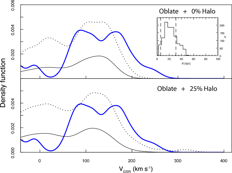
Figure 10: Comparison of the generalized histogram for the sample of stars in the VSS region (thick blue solid line) with the mean prediction of the LJM05 oblate model (black solid line). The dotted lines are the $\pm$3$\sigma$ bounds from the trials. The upper panel assumes no contribution from a smooth halo background while the lower panel assumes a contribution of 25 per cent. The inset shows the distance distribution of the model particles in the $\Lambda_{\odot}$ and $B_{\odot}$ range appropriate for the observed sample. The dashed lines indicate the distance range of the model particles used in the trials (6–31 kpc); the observed stars have distances between 13 and 21 kpc. It is evident that the observed sample contains significantly more stars at positive $V$${}_{\textrm{\scriptsize{GSR}}}$ values than predicted by the model.

To summarize broadly the information from our VSS region stars and those of DZV06 and Starkenburg et al. (2009) as regards the shape of the halo, the stars with $V$${}_{\textrm{\scriptsize{GSR}}}$ values between approximately –100 km s^-1 and –200 km s^-1 can be interpreted as old leading Sgr debris in the prolate halo model of LJM05, though the model points lie at somewhat larger distances than the observed stars. On the other hand, in the spherical and oblate models, the model points agree better in distance with the observed stars, the model velocities are substantially more negative than those observed. In contrast, the majority of the positive velocity stars agree in distance, velocity and in trend of velocity with $\Lambda_{\odot}$, with the predictions of the oblate model for old trailing Sgr debris. However, our simulations show that the predicted number of stars with positive $V$${}_{\textrm{\scriptsize{GSR}}}$ values is substantially less than the number observed. Nevertheless, for these positive $V$${}_{\textrm{\scriptsize{GSR}}}$ stars, the prolate model is the least satisfactory representation of the data. Thus, unlike the 21.5 h region where the support for the oblate model was strong, the VSS region provides somewhat contradictory information regarding the flattening of the dark halo.

3.3 Vivas et al.’s Sgr data

As a further attempt to investigate the shape of the halo potential, we compared the reported radial velocities of Vivas et al.’s (2005) (hereafter VZG05) 16 RRLs to LJM05’s models. These RRLs are located at a different angular separation from Sgr to our data, as shown in Fig. 11. The stars range in distance from 45 to 62 kpc with a mean of 53 kpc so that in Fig. 11 we highlight in red model particles with distances between 40 and 65 kpc. The stars cover a $B_{\odot}$ range from 9.6$\arcdeg$ to –8.3$\arcdeg$ so we are justified in plotting all $B_{\odot}$ values for the model particles. We also note that the group of 6 probable Sgr stars identified by Starkenburg et al. (2009) have locations, velocities and distances comparable to those of the VZG05 RRL stars. Consequently, these stars are also shown in Fig. 11. The $B_{\odot}$ values for these stars range between –11.5$\arcdeg$ and –6$\arcdeg$.

Upon comparing their data with those of Helmi (2004a) and Martínez-Delgado et al. (2004), VZG05 concluded that spherical and prolate models fit better than oblate models, though none of the fits are completely satisfactory. The comparison of LJM05’s models with the VZG05 and Starkenburg et al. (2009) data here reveals a similar conclusion. In Fig. 11, the prolate model is clearly the best fit, with all the stars except the two RRLs VZG05 identified as probable non-members appearing to belong to the leading stream (debris-c). We note, however, that while the spherical and oblate models produce progressively worse fits than the prolate model, they are not completely inconsistent with the data.

Figure 11: Radial velocities against $\Lambda_{\odot}$ from models with prolate (left), spherical (middle) and oblate (right) Galactic halo potentials (Law et al., 2005). Red dots denote simulated stars with heliocentric distances $d$ = 40–65 kpc while gray denotes stars at all other distances. All $B_{\odot}$ values are shown. Overplotted (filled circles) are values for the 16 hypothesized Sgr Stream RRLs observed by Vivas et al. (2005). The open circles represent the data for the Group 1 stars of Starkenburg et al. (2009), which are also likely associated with Sgr.

4 Metal Abundances

As described fully in Paper I, metallicities ([Fe/H]) were calculated for the type $ab$ RRLs using the Freeman & Rodgers (1975) method in which the pseudo-equivalent width (EW) of the Ca II K line, $W$(K), is plotted against the mean EW of the Balmer lines (H$\delta$, H$\gamma$ and H$\beta$), H3. RRLs trace out metallicity-dependent paths on this plot as they vary in phase, as calibrated by Layden (1994). The $W$(K)–H3 plot for the 21 type $ab$ RRLs in the 20 and 21.5 h Sgr regions (note that one RR$ab$ star was omitted since all observations corresponded to rising light phases) is shown in Fig. 12.

The values of [Fe/H] for these stars are listed in Table 1 and their distribution is shown in Fig. 13. Where more than one observation exists, the tabulated values were calculated by averaging the [Fe/H] values from the different phases (cf. Fig. 12). Based on the stars with multiple observations, the internal precision of a single [Fe/H] determination is 0.11 dex. For this sample, $\langle$[Fe/H]$\rangle$$=-1.79\pm 0.08$ dex on our [Fe/H] system with a dispersion of $\sigma$ = 0.38 dex (see Fig. 13). This mean value is in close agreement with VZG05’s measurement of $\langle$[Fe/H]$\rangle$= $-1.76$, $\sigma$ = 0.22 dex, for 14 QUEST RRLs in the Sgr tidal stream. As noted by VZG05, the observed $\langle$[Fe/H]$\rangle$ is consistent with the age-metallicity relation of the main body of Sgr (Layden & Sarajedini, 2000) if these RRLs are coeval with the oldest stellar population in the body, as they are indeed expected to be.

Figure 12: The pseudo-equivalent width of the Ca II K line, corrected for interstellar absorption, against the average width of H$\delta$, H$\gamma$ and H$\beta$ for the 21 type $ab$ RRLs in the Sgr region. Solid lines connect values for the same RRL observed at different phases. The dashed lines are the loci of stars having the indicated [Fe/H] value according to Layden’s (1994) calibration.

Figure 13: Generalized histogram of [Fe/H] (with kernel of 0.1 dex) for the 21 type $ab$ RRLs in the Sgr region.

We noted above that the 6 stars in the Sgr group (Group 1) of Starkenburg et al. (2009) lie in the same part of the Sgr stream as the VZG05 RRL stars. These red giants have a mean abundance of $\langle$[Fe/H]$\rangle$ = –1.68 $\pm$ 0.15, in excellent accord with that for the VZG05 stars. The observed abundance dispersion is 0.38 dex, which, given the large ($\sim$0.3 dex) abundance uncertainties, implies an intrinsic abundance disperion of $\sim$0.24 dex. This is again in good accord with the VZG05 results. The most metal-poor star in the group has [Fe/H] = –2.33 $\pm$ 0.31 while the most metal-rich has [Fe/H] = –1.29 $\pm$ 0.26 dex.

The [Fe/H] dispersion of our sample is larger than that found by VZG05 and that of the Starkenburg et al. (2009) group 1 stars, and is closer to the dispersion of $\sigma$ = 0.4 dex found by Kinman et al. (2000) for RRLs in the halo. It should be recalled, however, that our RRL sample likely includes field RRLs which are not part of the Sgr Stream. Contamination by such RRLs could thus inflate our estimate of the [Fe/H] dispersion for Sgr Stream stars. The dispersion could also be disproportionately influenced by outliers. We note that if the most metal rich and the most metal poor RRL (visible as the outermost, small bumps on Fig. 13) are excluded, the remaining stars have $\sigma$ = 0.23 dex and an abundance range of 0.8 dex, consistent with the values of VZG05 and for the Starkenburg et al. (2009) group 1 stars. Including those two stars, on the other hand, yields a much larger abundance range of 1.8 dex. A more rigorous way of reducing the effect of outlying, extreme values on the dispersion is to consider the inter-quartile range (IQR). We obtain IQR = 0.46 dex which is larger than that for VZG05’s data, IQR = 0.22 dex. It thus appears that the larger [Fe/H] dispersion in our Sgr Stream sample than in VZG05’s is not driven solely by outlying values. The differing abundance dispersions are perhaps unsurprising given that we are sampling a different part of the Sgr Stream than VZG05 and the group 1 stars of Starkenburg et al. (2009). Nevertheless the close agreement of the mean abundances for the three samples is intriguing.

Fig. 13 appears to show a hint of bimodal structure. However, a KS-test shows that the null hypothesis, namely that the sample (excluding the two outliers) is drawn from a single gaussian distribution with the sample mean and standard distribution, cannot be excluded with any significance: the probability that the null hypothesis is true is at least 20%. Similarly, if we isolate the stars that contribute to the two apparent peaks at [Fe/H] $\approx$ –2.0 and [Fe/H] $\approx$ –1.55, we find that the four 20 h stars are split between the two peaks 3 stars to 1, and the fifteen 21.5 h stars are split 8 stars to 7, i.e. the apparent abundance separation does not show any correlation with location. Further, for the 21.5 h stars, there is no difference in mean velocity or velocity dispersion between the groups separated by abundance.

The fact that the mean abundance we find for the 20 and 21.5 h RRLs agrees with that from VZG05 (and that from the Starkenburg et al. (2009) group 1 stars) in a different part of the Sgr stream raises the question of whether there is any pattern in mean [Fe/H] according to the part of the stream to which the RRLs belong. Indications of an age/metallicity gradient along the Sgr Stream have been observed, with stars stripped from Sgr on past perigalactic passages being older and more metal poor than the Sgr core and stars stripped more recently (Majewski et al., 2003; Martínez-Delgado et al., 2004; Bellazzini et al., 2006; Chou et al., 2007).

We thus searched for evidence of this abundance gradient by comparing the metallicities of RRLs in the 20 and 21.5 h regions which appear associated with the recent trailing debris stream (debris-a) to those likely associated with the older trailing debris stream (debris-b). The six RRLs in the former have $\langle$[Fe/H]$\rangle$ = $-1.76$, $\sigma=0.24$ dex while the seven stars in the latter have $\langle$[Fe/H]$\rangle$ = $-1.68$, $\sigma=0.48$ dex. Thus, we find no evidence for a correlation between location on the stream (and hence age of stripping) with abundance in our RRL sample.

A comparison of the recent results of Watkins et al. (2009) with those above might suggest a different conclusion. Watkins et al. (2009) listed a mean abundance of $\langle$[Fe/H]$\rangle$ = $-1.41\pm 0.19$ for a sample of likely Sgr RRLs identified from their analysis of the SDSS Stripe 82 region. In the context of the LJM05 models their RRL sample has a strong component from recent trailing debris (debris-a), especially if the halo potential is oblate. The majority of the abundance determinations in their sample come from analysis of the periods and light curve shapes derived from the photometry (Watkins et al., 2009). As such they are relatively more uncertain ($\sigma$([Fe/H]) $\approx$ 0.25 dex for the type ab, and 0.38 dex for the type c RRLs, Watkins et al. (2009)) than the direct spectroscopic determinations discussed here. Thus any comparison of the Watkins et al. (2009) mean abundance with those for the other RRL samples discussed here should be treated with caution. Nevertheless, given the association of the Watkins et al. (2009) sample with recent trailing debris, its higher mean metallicity compared to those of the other Sgr RRL samples might indicate the presence of an abundance gradient, not withstanding the results discussed in the previous paragraph. However, it must be recalled that RRLs are members of an old population and thus RRL samples do not necessarily represent an unbiased selection of stream members.

5 Discussion

The results presented in this paper impinge on two related issues. The first is the extent to which the velocities and distances of observed Sgr debris stars can be used in conjunction with the models of LJM05 to place constraints on the shape of the Galaxy’s dark halo. The second revolves around the interpretation of the overdensity in Virgo and its potential relation to Sgr debris.

The available observational data and the analysis presented here indicate that the Galactic halo substructure in the direction of Virgo is evidently quite complex. In Paper I we showed that considered as a spatial overdensity, the feature is large and diffuse and extends well to the south of the declination limits of the SDSS and of the QUEST survey (see also Keller et al., 2009). However, kinematically, there appear to be at least two distinct components that overlap spatially. One is defined by the group of RRLs with $\langle$$V$${}_{\textrm{\scriptsize{GSR}}}$$\rangle$ $\approx$ –160 km s^-1, which we identify as likely resulting from Sgr old leading debris (cf. Martínez-Delgado et al., 2007). This kinematic signature is also seen in the work of Newberg et al. (2007), Vivas et al. (2008) and pair 7 of Starkenburg et al. (2009).

At positive $V$${}_{\textrm{\scriptsize{GSR}}}$ values, there is concurrence in both spatial location, velocity, and velocity trend with orbital longitude of the combined observational sample of Paper I, Duffau et al. (2006) and Starkenburg et al. (2009) pair 8 with the predictions for Sgr old trailing debris in the LJM05 oblate model (cf. Fig. 9). This is suggestive that such debris may play a role in the (kinematically defined) feature labeled by Duffau et al. (2006) as the Virgo Stellar Stream. Such a possibility was foreshadowed by Martínez-Delgado et al. (2007). However, our simulations based on the LJM05 oblate model suggest strongly that Sgr old trailing debris cannot be the sole source of the positive $V$${}_{\textrm{\scriptsize{GSR}}}$ stars. Instead it is likely that there is at least one other independent structure that conspires with the Sgr debris to produce the observed excess. Clearly a detailed spatial and kinematic survey of a large region of sky is needed to clarify the situation. The SEKBO survey catalog alone provides a more than ample selection of RRL candidates in the VSS region for follow-up (cf. Paper I). We also have underway a survey targeting red giants in this region, which takes advantage of the wide field and large multiplex factor of the AAOmega multi-fiber spectrograph at Anglo-Australian Telescope.

As regards the shape of the halo potential, the existence of a distinct group of RRLs with large negative $V$${}_{\textrm{\scriptsize{GSR}}}$ values in the 21.5 h sample strongly favors the oblate model of LJM05. However, the negative $V$${}_{\textrm{\scriptsize{GSR}}}$ stars in the VSS region, interpreted as Sgr old leading debris, and the more distant samples of Vivas et al. (2005) and Starkenburg et al. (2009) group 1, tell a different story in which prolate models are favored. These findings echo those of LJM05, wherein trailing data favor oblate models and leading data favor prolate models, and reinforce the conclusion that the issue of dark halo shape cannot be definitively resolved with current models of the Sgr disruption.

LJM05 suggest that an evolution of the orbital parameters of Sgr over several Gyr may need to be considered. In addition, the Sgr dwarf itself may need to be modeled as a two component system, in which the dark matter is bound more loosely than the baryons. Warnick et al.’s (2008) N-body simulations of satellite disruption within “live” (cosmological) host halos suggest that the situation may be far more complicated than previously envisioned. Their preliminary studies find little correlation between debris properties and host halo properties such as shape. They note that the host dark halo undergoes a complex mass accretion history and also comment that it cannot be easily modeled as a simple ellipsoid due to the wealth of substructure present. In contrast, Siegal-Gaskins & Valluri (2008) investigate the effects of dark matter substructure on tidal streams and find that halo shape and orbital path play a much more important role in the large-scale structure of the debris. However, they do note that substructure increases the clumpiness of the debris and changes the location of certain sections compared to the predictions from a smooth halo model. This could add an extra complication to studies such as the current one, where attempts are made to compare tidal debris models with data.

6 Conclusions

Analysis of follow-up spectroscopy of 26 photometrically confirmed RRLs from a candidate list based on SEKBO survey data reveals a radial velocity distribution which does not appear consistent with a smooth halo population. Based on their location, the RRLs are likely to be associated with debris from the disrupting Sgr dwarf galaxy. The 21 type $ab$ RRLs in the 20 and 21.5 h regions have $\langle$[Fe/H]$\rangle$ = $-1.79\pm 0.08$ on our system and a large abundance range of $\sim$1.8 dex ($\sigma$ = 0.35), or 0.8 dex ($\sigma$ = 0.23) omitting the two most extreme values. The interquartile range is 0.46 dex. While the abundance spread in our data appears to be larger, the mean metallicity is consistent with that of Vivas et al. (2005) for Sgr tidal debris RRLs, and that of the group 1 (Sgr) red giants from Starkenburg et al. (2009), which lie in a different part of the Sgr debris stream. The mean abundance for the Sgr RRLs in the Watkins et al. (2009) sample, however, is apparently somewhat higher, though based on a different technique.

A comparison of the radial velocities with those predicted by the models of Law et al. (2005) supports the hypothesis that the observed RRLs predominantly belong to the Sgr Stream. In the 21.5 h region, a group of stars with highly negative radial velocities ($V$${}_{\textrm{\scriptsize{GSR}}}$$\sim-175$ km s^-1) is consistent with predictions for old trailing debris when the Galactic halo potential is modeled as oblate. In contrast, the prolate model does not predict any significant Sgr debris at the $\Lambda_{\odot}$ and $B_{\odot}$ of the observed sample, indicating that it requires modification if it is to be viable. The observations also seem to require that the recent trailing debris stream has a larger spread in $B_{\odot}$ than predicted by any of the models.

Comparison of radial velocities of VSS region RRLs with the Sgr debris models reveals intriguing similarities in trends with $\Lambda_{\odot}$. Together with the evidence of spatial coincidence of these stars with the predicted debris streams, our results provide observational support for Martínez-Delgado et al.’s (2007) proposition that Sgr debris is in fact at least partially responsible for the overdensity in Virgo. In particular, it seems likely that the stars with large negative $V$${}_{\textrm{\scriptsize{GSR}}}$ values are best interpreted as old leading debris. However, at least in the context of the LJM05 models, it appears unlikely that the feature at $V$${}_{\textrm{\scriptsize{GSR}}}$ $\approx$ 100 km s^-1, the VSS, can be explained solely as Sgr old trailing debris. While Sgr old trailing debris may make a contribution, the (kinematically defined) VSS is apparently a structure in the halo of the Galaxy independent of Sgr debris.

Considering all the data sets for suspected Sgr Stream members presented in this paper, we find further evidence for Law et al.’s observation that trailing debris is best fit by oblate models while leading debris favors prolate models. That is, we are in agreement with Law et al.’s conclusion that no single orbit and/or potential can fit all the observed data. Further modeling is needed to investigate higher order effects such as orbital evolution. To this end, data from RRLs may prove useful as these old stars could potentially have been stripped from Sgr several orbits ago. It may also be necessary for models to include the possibility that the flattening of the halo varies with radius (e.g. Bailin & Steinmetz, 2005) or that it is triaxial (cf. Law et al., 2009). The high accuracy of determined distances to RRLs provides an extra incentive to use these stars as probes of Sgr debris.

References

- Bailin & Steinmetz (2005) Bailin, J., & Steinmetz, M. 2005, ApJ, 627, 647
- Bell et al. (2008) Bell, E. F., Zucker, D. B., Belokurov, V., Sharma, S., Johnston, K. V., Bullock, J. S., Hogg, D. W., Jahnke, K., de Jong, J. T. A., Beers, T. C., Evans, N. W., Grebel, E. K., Ivezić, Ž., Koposov, S. E., Rix, H.-W., Schneider, D. P., Steinmetz, M., & Zolotov, A. 2008, ApJ, 680, 295
- Bellazzini et al. (2006) Bellazzini, M., Newberg, H. J., Correnti, M., Ferraro, F. R., & Monaco, L. 2006, A&A, 457, L21
- Belokurov et al. (2006) Belokurov, V., Zucker, D. B., Evans, N. W., Gilmore, G., Vidrih, S., Bramich, D. M., Newberg, H. J., Wyse, R. F. G., Irwin, M. J., Fellhauer, M., Hewett, P. C., Walton, N. A., Wilkinson, M. I., Cole, N., Yanny, B., Rockosi, C. M., Beers, T. C., Bell, E. F., Brinkmann, J., Ivezić, Ž., & Lupton, R. 2006, ApJ, 642, L137
- Brown et al. (2005) Brown, W. R., Geller, M. J., Kenyon, S. J., Kurtz, M. J., Allende Prieto, C., Beers, T. C., & Wilhelm, R. 2005, AJ, 130, 1097
- Chou et al. (2007) Chou, M.-Y., Majewski, S. R., Cunha, K., Smith, V. V., Patterson, R. J., Martínez-Delgardo, D., Law, D. R., Crane, J. D., Muñoz, R. R., Garcia López, R., Geisler, D., & Skrutskie, M. F. 2007, ApJ, 670, 346
- Dohm-Palmer et al. (2001) Dohm-Palmer, R. C., Helmi, A., Morrison, H., Mateo, M., Olszewski, E. W., Harding, P., Freeman, K. C., Norris, J., & Shectman, S. A. 2001, ApJL, 555, L37
- Duffau et al. (2006) Duffau, S., Zinn, R., Vivas, A. K., Carraro, G., Méndez, R. A., Winnick, R., & Gallart, C. 2006, ApJ, 636, L97 (DZV06)
- Fellhauer et al. (2006) Fellhauer, M., Belokurov, V., Evans, N. W., Wilkinson, M. I., Zucker, D. B., Gilmore, G., Irwin, M. J., Bramich, D. M., Vidrih, S., Wyse, R. F. G., Beers, T. C., & Brinkmann, J. 2006, ApJ, 651, 167
- Freeman & Rodgers (1975) Freeman, K. C. & Rodgers, A. W. 1975, ApJ, 201, L71
- Helmi (2004a) Helmi, A. 2004a, MNRAS, 351, 643
- Helmi (2004b) —. 2004b, ApJ, 610, L97
- Helmi & White (2001) Helmi, A. & White, S. D. M. 2001, MNRAS, 323, 529
- Ibata et al. (2001) Ibata, R., Lewis, G. F., Irwin, M., Totten, E., & Quinn, T. 2001, ApJ, 551, 294
- Ibata et al. (1994) Ibata, R. A., Gilmore, G., & Irwin, M. J. 1994, Nature, 370, 194
- Ivezić et al. (2000) Ivezić, Ž., Goldston, J., Finlator, K., Knapp, G. R., Yanny, B., McKay, T. A., Amrose, S., Krisciunas, K., Willman, B., Anderson, S., Schaber, C., Erb, D., Logan, C., Stubbs, C., Chen, B., Neilsen, E., Uomoto, A., Pier, J. R., Fan, X., Gunn, J. E., Lupton, R. H., Rockosi, C. M., Schlegel, D., Strauss, M. A., Annis, J., Brinkmann, J., Csabai, I., Doi, M., Fukugita, M., Hennessy, G. S., Hindsley, R. B., Margon, B., Munn, J. A., Newberg, H. J., Schneider, D. P., Smith, J. A., Szokoly, G. P., Thakar, A. R., Vogeley, M. S., Waddell, P., Yasuda, N., & York, D. G. 2000, AJ, 120, 963
- Johnston et al. (1999) Johnston, K. V., Majewski, S. R., Siegel, M. H., Reid, I. N., & Kunkel, W. E. 1999, AJ, 118, 1719
- Jurić et al. (2008) Jurić, M., Ivezić, Ž., Brooks, A., Lupton, R. H., Schlegel, D., Finkbeiner, D., Padmanabhan, N., Bond, N., Sesar, B., Rockosi, C. M., Knapp, G. R., Gunn, J. E., Sumi, T., Schneider, D. P., Barentine, J. C., Brewington, H. J., Brinkmann, J., Fukugita, M., Harvanek, M., Kleinman, S. J., Krzesinski, J., Long, D., Neilsen, Jr., E. H., Nitta, A., Snedden, S. A., & York, D. G. 2008, ApJ, 673, 864
- Keller et al. (2008) Keller, S. C., Murphy, S., Prior, S., Da Costa, G., & Schmidt, B. 2008, ApJ, 678, 851 (KMP08)
- Keller et al. (2009) Keller, S. C., Da Costa, G. S., & Prior, S. L. 2009, MNRAS, 394, 1045
- Kinman et al. (2000) Kinman, T., Castelli, F., Cacciari, C., Bragaglia, A., Harmer, D., & Valdes, F. 2000, A&A, 364, 102
- Kundu et al. (2002) Kundu, A., Majewski, S. R., Rhee, J., Rocha-Pinto, H. J., Polak, A. A., Slesnick, C. L., Kunkel, W. E., Johnston, K. V., Patterson, R. J., Geisler, D., Gieren, W., Seguel, J., Smith, V. V., Palma, C., Arenas, J., Crane, J. D., & Hummels, C. B. 2002, ApJ, 576, L125
- Law et al. (2005) Law, D. R., Johnston, K. V., & Majewski, S. R. 2005, ApJ, 619, 807 (LJM05)
- Law et al. (2009) Law, D. R., Majewski, S. R., & Johnston, K. V. 2009, ApJ, accepted (arXiv:0908.3187)
- Layden (1994) Layden, A. C. 1994, AJ, 108, 1016
- Layden & Sarajedini (2000) Layden, A. C. & Sarajedini, A. 2000, AJ, 119, 1760
- Majewski et al. (1999) Majewski, S. R., Siegel, M. H., Kunkel, W. E., Reid, I. N., Johnston, K. V., Thompson, I. B., Landolt, A. U., & Palma, C. 1999, AJ, 118, 1709
- Majewski et al. (2003) Majewski, S. R., Skrutskie, M. F., Weinberg, M. D., & Ostheimer, J. C. 2003, ApJ, 599, 1082
- Martínez-Delgado et al. (2004) Martínez-Delgado, D., Gómez-Flechoso, M. Á., Aparicio, A., & Carrera, R. 2004, ApJ, 601, 242
- Martínez-Delgado et al. (2007) Martínez-Delgado, D., Peñarrubia, J., Jurić, M., Alfaro, E. J., & Ivezić, Z. 2007, ApJ, 660, 1264
- Newberg et al. (2007) Newberg, H. J., Yanny, B., Cole, N., Beers, T. C., Re Fiorentin, P., Schneider, D. P., & Wilhelm, R. 2007, ApJ, 668, 221
- Newberg et al. (2003) Newberg, H. J., Yanny, B., Grebel, E. K., Hennessy, G., Ivezić, Ž., Martinez-Delgado, D., Odenkirchen, M., Rix, H.-W., Brinkmann, J., Lamb, D. Q., Schneider, D. P., & York, D. G. 2003, ApJ, 596, L191
- Newberg et al. (2002) Newberg, H. J., Yanny, B., Rockosi, C., Grebel, E. K., Rix, H.-W., Brinkmann, J., Csabai, I., Hennessy, G., Hindsley, R. B., Ibata, R., Ivezić, Z., Lamb, D., Nash, E. T., Odenkirchen, M., Rave, H. A., Schneider, D. P., Smith, J. A., Stolte, A., & York, D. G. 2002, ApJ, 569, 245
- Prior et al. (2009) Prior, S. L., Da Costa, G., Keller, S. C., & Murphy, S. J. 2009, ApJ, 691, 306 (Paper I)
- Sarajedini & Layden (1995) Sarajedini, A., & Layden, A. C., 1995, AJ, 109, 1086SL9
- Searle & Zinn (1978) Searle, L. & Zinn, R. 1978, ApJ, 225, 357
- Siegal-Gaskins & Valluri (2008) Siegal-Gaskins, J. M. & Valluri, M. 2008, ApJ, 681, 40
- Sirko et al. (2004) Sirko, E., Goodman, J., Knapp, G. R., Brinkmann, J., Ivezić, Ž., Knerr, E. J., Schlegel, D., Schneider, D. P., & York, D. G. 2004, AJ, 127, 899
- Springel et al. (2006) Springel, V., Frenk, C. S., & White, S. D. M. 2006, Nature, 440, 1137
- Starkenburg et al. (2009) Starkenburg, E., Helmi, A., Morrison, H. L., Harding, P., van Woerden, H., Mateo, M., Olszewski, E. W., Sivarani, T., Norris, J. E., Freeman, K. C., Shectman, S. A., Dohm-Palmer, R. C., Frey, L., & Oravetz, D. 2009, ApJ, 698, 567
- Totten & Irwin (1998) Totten, E. J. & Irwin, M. J. 1998, MNRAS, 294, 1
- Vivas et al. (2008) Vivas, A. K., Jaffé, Y. L., Zinn, R., Winnick, R., Duffau, S., & Mateu, C. 2008, AJ, 136, 1645
- Vivas & Zinn (2006) Vivas, A. K. & Zinn, R. 2006, AJ, 132, 714
- Vivas et al. (2004) Vivas, A. K., Zinn, R., Abad, C., Andrews, P., Bailyn, C., Baltay, C., Bongiovanni, A., Briceño, C., Bruzual, G., Coppi, P., Della Prugna, F., Ellman, N., Ferrín, I., Gebhard, M., Girard, T., Hernandez, J., Herrera, D., Honeycutt, R., Magris, G., Mufson, S., Musser, J., Naranjo, O., Rabinowitz, D., Rengstorf, A., Rosenzweig, P., Sánchez, G., Sánchez, G., Schaefer, B., Schenner, H., Snyder, J. A., Sofia, S., Stock, J., van Altena, W., Vicente, B., & Vieira, K. 2004, AJ, 127, 1158
- Vivas et al. (2001) Vivas, A. K., Zinn, R., Andrews, P., Bailyn, C., Baltay, C., Coppi, P., Ellman, N., Girard, T., Rabinowitz, D., Schaefer, B., Shin, J., Snyder, J., Sofia, S., van Altena, W., Abad, C., Bongiovanni, A., Briceño, C., Bruzual, G., Della Prugna, F., Herrera, D., Magris, G., Mateu, J., Pacheco, R., Sánchez, G., Sánchez, G., Schenner, H., Stock, J., Vicente, B., Vieira, K., Ferrín, I., Hernandez, J., Gebhard, M., Honeycutt, R., Mufson, S., Musser, J., & Rengstorf, A. 2001, ApJ, 554, L33
- Vivas et al. (2005) Vivas, A. K., Zinn, R., & Gallart, C. 2005, AJ, 129, 189
- Warnick et al. (2008) Warnick, K., Knebe, A., & Power, C. 2008, MNRAS, 385, 1859
- Watkins et al. (2009) Watkins, L. L., Evans, N. E., Belokurov, V., Smith, M. C., Hewtt, P. C., Bramich, D. M., Gilmore, G. F., Irwin, M. J., Vidrih, S., Wyrzykowski, L., & Zucker, D. B. 2009, MNRAS, in press (arXiv:0906.0498)