Local correlations of mixed two-qubit states

Abstract

The quantum probability distribution arising from single-copy von Neumann measurements on an arbitrary two-qubit state is decomposed into the local and nonlocal parts, in the approach of Elitzur, Popescu and Rohrlich [A. Elitzur, S. Popescu, and D. Rohrlich, Phys. Lett. A 162, 25 (1992)]. A lower bound of the local weight is proved being connected with the concurrence of the state $p_{L}^{\max}=1-\mathcal{C}(\rho)$. The local probability distributions for two families of mixed states are constructed independently, which accord with the lower bound.

I Introduction

Entanglement and nonlocality are two fundamental concepts in quantum description of nature, which are closely interconnected but not identical EPR ; Bell ; Werner1989 . The former depicts the nonseparability of the state of a composite quantum system EPR , while the latter is characterized by violation of a Bell inequality Bell , which means the local measurement outcomes of the state cannot be described by a local hidden variables (LHV) model. It has been proved that all pure entangled states violate such an inequality and, consequently, are nonlocal Gisin1991 . But Werner Werner1989 has shown a family of mixed entangled states (called Werner states now) can be described by a LHV model. The two concepts are not only the fundamental features of quantum theory, but also the crucial resources in quantum information Book ; code ; key ; key2 .

To quantify the degree to which a state is entangled, several measures have been proposed, such as entanglement of formation EOF ; Wootters97 ; Wootters98 , entanglement of distillation EOD , relative entropy of entanglement REE , negativity NEG ; NEG1 , and so on. For two-qubit systems, the entanglement of formation is equivalent to a computable quantity, which is referred to as concurrence Wootters97 ; Wootters98 . The concurrence of a pure two-qubit state $|\psi\rangle=c_{1}|00\rangle+c_{2}|01\rangle+c_{3}|10\rangle+c_{4}|11\rangle$ is given by

$$\mathcal{C}(|\psi\rangle)=2|c_{1}c_{4}-c_{2}c_{3}|.$$ (1)

The pure state is equivalent to

$$|\psi(\theta)\rangle=\cos\theta|00\rangle+\sin\theta|11\rangle,\ \ \ \theta\in[0,\pi/4],$$ (2)

under local unitary (LU) transformations Book , with concurrence $\mathcal{C}(|\psi(\theta)\rangle)=2\cos\theta\sin\theta=\sin 2\theta$. For a mixed state, the concurrence is defined as the average concurrence of the pure states of the decomposition, minimized over all decompositions of $\rho=\sum_{j}p_{j}|\psi_{j}\rangle\langle\psi_{j}|$,

$$\mathcal{C}(\rho)=\min\sum_{j}p_{j}\mathcal{C}(|\psi_{j}\rangle).$$ (3)

It can be expressed explicitly as Wootters97 ; Wootters98

$$\mathcal{C}(\rho)=\max\biggr{\{}0,\sqrt{\lambda_{1}}-\sqrt{\lambda_{2}}-\sqrt{\lambda_{3}}-\sqrt{\lambda_{4}}\biggr{\}},$$ (4)

in which $\lambda_{1},...,\lambda_{4}$ are the eigenvalues of the operator $R=\rho(\sigma_{y}\otimes\sigma_{y})\rho^{*}(\sigma_{y}\otimes\sigma_{y})$ in decreasing order and $\sigma_{y}$ is the second Pauli matrix.

The correlation in a bipartite quantum system is characterized by the probability distribution $P_{Q}(\alpha,\beta|\mathbf{a},\mathbf{b})$ of the outcomes $\alpha$ and $\beta$, corresponding to the measurements labeled by $\mathbf{a}$ and $\mathbf{b}$ on the two subsystems respectively. It is called local, if the probability distribution can be simulated by a LHV model. Namely, there exists a shared classical variable $\lambda$ distributed with probability measure $\mu$ such that

$$P_{Q}(\alpha,\beta|\mathbf{a},\mathbf{b})=\int d\mu(\lambda)P(\alpha|\mathbf{a},\lambda)P(\beta|\mathbf{b},\lambda),$$ (5)

where $P(\alpha|\mathbf{a},\lambda)$ and $P(\beta|\mathbf{b},\lambda)$ are the local response functions of the two observers. The form of the distribution in Eq. (5) leads to a set of constraints on the local correlation (Bell-type inequalities), for any fixed number of measurements on each subsystem. Therefore, Bell inequality violation is a sufficient condition of quantum nonlocality.

Elitzur, Popescu, and Rohrlich (EPR2) EPR2 discuss the local and nonlocal contents of nonlocal probability distributions [see Eq. (6)] from a different point of view. Actually, EPR2 approach can be abstractly interpreted to answer such a question: whether an alternative description of nature is valid. Since the original work of EPR2 appeared, few papers generalized it in depth. Recently, as the approach is related to a more noticeable question, the simulation of quantum correlations with other resource, it attracted someone’s attention again. Barrett et. al gave an upper bound of the weight of local component in $d\times d$ system Barrett2006 . In his recent work Scarani2008 , Scarani reviewed the previous results and decomposed the quantum correlation $P_{Q}$ corresponding to von Neumann measurements performed on the pure state (2) into a mixture of a local correlation $P_{L}$ and a nonlocal correlation $P_{NL}$

$$P_{Q}=p_{L}(\theta)P_{L}+[1-p_{L}(\theta)]P_{NL},$$ (6)

in EPR2 approach. Scarani’s construction of the local probability distribution $P_{L}$ leads to

$$p_{L}(\theta)=1-\sin 2\theta,$$ (7)

which is an improved lower bound of $p_{L}^{\max}(\theta)$ on the original result $p_{L}^{\max}(\theta)\geq(1-\sin 2\theta)/4$ given by EPR2. Here, $p_{L}^{\max}(\theta)$ denotes the maximum weight of the local component in Eq. (6). Further more, he presented an upper bound for $p_{L}^{\max}(\theta)$ on the family of pure two-qubit states and the first example of a lower bound on the local content of pure two-qutrit states.

It is interesting to note that the proportion of nonlocal correlation $P_{NL}$ in Scarani’s construction is nothing but the concurrence of $|\psi(\theta)\rangle$, $1-p_{L}(\theta)=\sin 2\theta$. The main aim of this paper is to show this result can be generalized straightway to the mixed states case. Namely, we present a construction of $P_{L}$ for arbitrary states $\rho$ of two qubits, corresponding to the local weight $p_{L}(\rho)=1-\mathcal{C}(\rho)$. The construction will be proved as a theorem in Sec. II. In addition, we will give the EPR2 decompositions of some typical states in quantum information, such as the Generalized Werner state RhoWG and the mixture of a Bell state and a mixed diagonal state, of which Werner state and maximally entangled mixed states $\rho_{MEMS}$ MEMS are two spacial cases. Conclusion will be made in the last section.

II EPR2 decompositions of Mixed Two-Qubit states

II.1 General Results

The probality that the local von Neumann measurements labeled by unit vectors $\mathbf{a}$ and $\mathbf{b}$ performed on the two qubits with state $\rho$ lead to the outcomes ($\alpha$, $\beta$) is

$$P_{Q}(\alpha,\beta|\rho;\mathbf{a},\mathbf{b})=\mathrm{Tr}(\Pi_{A}\otimes\Pi_{B}\rho),$$ (8)

with $\alpha,\beta=\pm 1$. Here, the projectors are given by

$$\Pi_{A}=\frac{1}{2}(\mathbf{1}+\vec{\mathbf{\sigma}}\cdot\mathbf{A}),$$

$$\Pi_{B}=\frac{1}{2}(\mathbf{1}+\vec{\mathbf{\sigma}}\cdot\mathbf{B}),$$ (9)

where $\mathbf{1}$ is the $2\times 2$ unit matrix, $\vec{\sigma}=(\sigma_{x},\sigma_{y},\sigma_{z})$ are the Pauli matrices in vector notation, and $\mathbf{A}=\alpha\mathbf{a}$ and $\mathbf{B}=\alpha\mathbf{b}$ are unit vectors. Then, the quantum probability distribution of the pure state $|\psi(\theta)\rangle$ can be obtained easily

$$P_{Q}(\theta)=\frac{1}{4}[1+c(A_{z}+B_{z})+A_{z}B_{z}+s(A_{x}B_{x}-A_{y}B_{y})],\ \$$ (10)

where $c=\cos 2\theta$ and $s=\sin 2\theta$ as denoted in Scarani2008 . Scarani improved the local probability distribution on EPR2’s original construction to

$$P_{L}=\frac{1}{4}[1+f(A_{z})][1+f(B_{z})],$$ (11)

with the function $f(x)=\mathrm{sgn}(x)\min(1,\frac{c}{1-s}|x|)$. This keeps the product form in EPR2 and leads to $p_{L}=1-s=1-\mathcal{C}(|\psi(\theta)\rangle)$.

Whereas, the product form construction of $P_{L}$ is obviously not optimal for mixed states because of the presence of classical correlation. A simple example is the separable state $\rho_{s}=(|00\rangle\langle 00|+|11\rangle\langle 11|)/2$, whose quantum probability distribution $P_{Q}(\rho_{s})=(1+A_{z}B_{z})/4$ should be completely local. One can easily find the following equation is self-contradictory,

$$P_{Q}(\rho_{s})=\frac{1}{4}(1+f_{A})(1+f_{B}),\ \ f_{A},f_{B}\in[-1,1],$$ (12)

if $f_{A}$ and $f_{B}$ are requested to be odd functions of $\mathbf{A}$ and $\mathbf{B}$ respectively. Actually, a straightforward construction of the local correlation of $\rho_{s}$ is

$$P_{L}(\rho_{s}) = \frac{1}{2}F^{+}(A_{z})F^{+}(B_{z})+\frac{1}{2}F^{-}(A_{z})F^{-}(B_{z})$$ (13)

$$= P_{Q}(\rho_{s}),$$

with $F^{\pm}(x)=\frac{1}{2}(1\pm x)$. It contains a two-outcomes random variable with equiprobability as the LHV. The following results will show the local weight of an arbitrary two-qubit state satisfies $p_{L}=1-\mathcal{C}(\rho)$, if we choose the local probability distribution with a discrete LHV as

$$P_{L}=\sum_{i}\mu_{i}p_{i}(\mathbf{A})q_{i}(\mathbf{B}),$$ (14)

where $\mu_{i},p_{i}(\mathbf{A}),q_{i}(\mathbf{B})\in[0,1]$ are probabilities satisfying $\sum_{i}\mu_{i}=1$, $p_{i}(\mathbf{A})+p_{i}(\mathbf{-A})=1$ and $q_{i}(\mathbf{B})+q_{i}(\mathbf{-B})=1$.

Theorem 1. The local content of the probability distribution for a two-qubit state $\rho$ has a lower bound $p_{L}^{\max}(\rho)\geq 1-\mathcal{C}(\rho)$.

Proof. According to the procedure given by Wootters Wootters98 , one can always obtain a decomposition $\{|\phi_{i}\rangle\}$ minimizing the average concurrence in Eq. (3), $\rho=\sum_{i}t_{i}|\phi_{i}\rangle\langle\phi_{i}|$, in which $\sum_{i}t_{i}=1$ and all the elements have the same value of concurrence as the mixed state $\rho$. The elements are equivalent under LU transformation to the same state in the form of Eq. (2)

$$|\phi_{i}\rangle\ =U^{A}_{i}\otimes U^{B}_{i}|\psi(\theta)\rangle,$$ (15)

with the concurrence $\mathcal{C}(|\psi(\theta)\rangle)=\mathcal{C}(\rho)$.

Denote the unit vectors by $\mathbf{A}^{(i)}$ and $\mathbf{B}^{(i)}$, which satisfy $\vec{\mathbf{\sigma}}\cdot\mathbf{A}^{(i)}=U^{A{\dagger}}_{i}\vec{\mathbf{\sigma}}\cdot\mathbf{A}U^{A}_{i}$ and $\vec{\mathbf{\sigma}}\cdot\mathbf{B}^{(i)}=U^{B{\dagger}}_{i}\vec{\mathbf{\sigma}}\cdot\mathbf{B}U^{B}_{i}$. The quantum probability distribution is straightforward to obtain

$$P_{Q}(\rho)=\sum_{i}t_{i}P_{Q}^{(i)},$$ (16)

where $P_{Q}^{(i)}=\langle\psi(\theta)|\Pi^{(i)}_{A}\otimes\Pi^{(i)}_{B}|\psi(\theta)\rangle$ with $\Pi^{(i)}_{A}=\frac{1}{2}[\mathbf{1}+\vec{\mathbf{\sigma}}\cdot\mathbf{A}^{(i)}]$ and $\Pi^{(i)}_{B}=\frac{1}{2}[\mathbf{1}+\vec{\mathbf{\sigma}}\cdot\mathbf{B}^{(i)}]$. Each $P_{Q}^{(i)}$ can be decomposed in Scarani’s approach as

$$P_{Q}^{(i)}=[1-\mathcal{C}(\rho)]P_{L}^{(i)}+\mathcal{C}(\rho)P_{NL}^{(i)},$$ (17)

where $P_{L}^{(i)}$ is defined in the form of Eq. (11) with $\mathbf{A}^{(i)}$ being substituted for $\mathbf{A}$ and $\mathbf{B}^{(i)}$ for $\mathbf{B}$. A natural construction of the local probability distribution is $P_{L}(\rho)=\sum_{i}t_{i}P_{L}^{(i)}$, taking the form in Eq. (14). Then, one can obtain

$$P_{Q}(\rho)=[1-\mathcal{C}(\rho)]P_{L}(\rho)+\mathcal{C}(\rho)\sum_{i}t_{i}P_{NL}^{(i)},$$ (18)

which ends the proof. $\square$

Since the procedure given by Wootters Wootters98 to derive the optimal decomposition in Eq. (3) is effective but not easy to implement, we give the EPR2 decompositions of two families of typical mixed states in the following parts of this section. These are constructed directly, independent of the process presented above.

II.2 Werner State & Generalized Werner State

The Werner state Werner1989 takes the form as

$$\rho_{W}=x|\psi^{+}\rangle\langle\psi^{+}|+(1-x)\frac{\mathbf{1}\otimes\mathbf{1}}{4},\ \ \ x\in[0,1],$$ (19)

where $|\psi^{+}\rangle=[|00\rangle+|11\rangle]/\sqrt{2}$ is one of the Bell basis. The concurrence $\mathcal{C}(\rho_{W})=\max\{0,(3x-1)/2\}$. And its quantum probability distribution is given by

$$P_{Q}(\rho_{W})=\frac{1}{4}[1+x(A_{z}B_{z}+A_{x}B_{x}-A_{y}B_{y})].$$ (20)

When $x=1/3$, $\rho_{W}$ is separable, and $P_{Q}(\rho_{W})$ can be represented as a local form

$$P_{L}^{1/3}(\rho_{W}) = \frac{1}{6}[F^{+}(A_{z})F^{+}(B_{z})+F^{-}(A_{z})F^{-}(B_{z})+F^{+}(A_{x})F^{+}(B_{x})$$ (21)

$$+F^{-}(A_{x})F^{-}(B_{x})+F^{+}(A_{y})F^{-}(B_{y})+F^{-}(A_{y})F^{+}(B_{y})]$$

$$= P_{Q}(\rho_{W})|_{x=1/3}.$$

If we define the local distribution as

$$P_{L}(\rho_{W})=\left\{\begin{array}[]{lr}P_{L}^{1/3}(\rho_{W}),&x\geq 1/3\;;\\ 3xP_{L}^{1/3}(\rho_{W})+(1-3x)\frac{1}{4},&x<1/3\;;\end{array}\right.$$ (24)

it is easy to prove $P_{Q}(\rho_{W})=P_{L}(\rho_{W})$ for $x<1/3$ and $P_{Q}(\rho_{W})/P_{L}(\rho_{W})\geq\frac{3}{2}(1-x)$ for $x\geq 1/3$. The minimum of the radio occurs when the unit vectors $\mathbf{A}\cdot\mathbf{B^{\prime}}=-1$ with $\mathbf{B^{\prime}}=(B_{x},-B_{y},B_{z})$. This indicates the local content of Werner state $p_{L}(\rho_{W})=1-\mathcal{C}(\rho_{W})$ corresponding to the construction of $P_{L}(\rho_{W})$ in Eq. (24).

However, a better bound can be obtained easily based on the fact that an entangled Werner state may admit a LHV model. In the seminal work of Werner Werner1989 , he constructed a LHV model of the states (19) for $x\leq 1/2$ under von Neumann measurements. This result has been extended to general measurements WernerState2002 and more parties WernerState2006 . In PhysRevA.73.062105 , Acín et. al. proved the quantum probability distribution (20) is local when the parameter $x\leq x_{c}=0.6595$ under von Neumann measurements. Therefore, we can replace the demarcation point $1/3$ by $x_{c}$, and define the separable function (24) using $P_{L}^{x_{c}}(\rho_{W})=P_{Q}(\rho_{W})|_{x=x_{c}}$ instead of $P_{L}^{1/3}(\rho_{W})$. Choosing the combinatorial coefficients in Eq. (24) as $\{x/x_{c},1-x/x_{c}\}$, we obtain a better bound $p^{{}^{\prime}}_{L}(\rho_{W})=1-\mathcal{C}^{{}^{\prime}}(\rho_{W})$ with $\mathcal{C}^{{}^{\prime}}(\rho_{W})=\max\{0,(x-x_{c})/(1-x_{c})\}$. Whereas, it is difficult to extended this result to any more general two-qubit states. In the following paragraph, we will show the construction of $P_{L}(\rho_{W})$ in Eqs. (21) and (24) can be generalized to treat the states in Eq. (25).

A family of generalized Werner state RhoWG is given by

$$\rho_{GW}=x|\psi(\theta)\rangle\langle\psi(\theta)|+(1-x)\frac{\mathbf{1}\otimes\mathbf{1}}{4},$$ (25)

which is the mixture of the pure state (2) with the completely random state. Its concurrence is $\mathcal{C}(\rho_{GW})=\max\{0,[(1+2s)x-1]/2\}$, and quantum correlation can be obtained

$$P_{Q}(\rho_{GW})=\frac{1}{4}\{1+x[cA_{z}+cB_{z}+A_{z}B_{z}+s(A_{x}B_{x}-A_{y}B_{y})]\},$$ (26)

with $s$ and $c$ taking the definition in Eq. (10). As the treatment of Werner state, we start from the critical value of $x_{c}=1/(1+2s)$, for which Eq. (26) is local obviously

$$P_{L}^{x_{c}}(\rho_{GW}) = \frac{x_{c}}{2}\{c_{+}F^{+}(A_{z})F^{+}(B_{z})+c_{-}F^{-}(A_{z})F^{-}(B_{z})$$ (27)

$$\ \ \ +sF^{+}(A_{x})F^{+}(B_{x})+sF^{-}(A_{x})F^{-}(B_{x})$$

$$\ \ \ +sF^{+}(A_{y})F^{-}(B_{y})+sF^{-}(A_{y})F^{+}(B_{y})\}$$

$$= P_{Q}(\rho_{GW})|_{x=x_{c}},$$

where $c_{\pm}=1\pm c$. When $x<x_{c}$, one can choose

$$P_{L}(\rho_{GW}) = (1+2s)xP_{L}^{x_{c}}(\rho_{GW})+[1-(1+2s)x]\frac{1}{4}$$ (28)

$$= P_{Q}(\rho_{GW})$$

For the entangled region $x>x_{c}$, an appropriate construction of local distribution is given by the linear combination

$$P_{L}(\rho_{GW})=kP_{L}+(1-k)P_{L}^{x_{c}}(\rho_{GW}),$$ (29)

where $P_{L}$ is the construction for pure state in Eq. (11), and $k=\frac{(1-s)[(1+2s)x-1]}{s[3-(1+2s)x]}\in[0,1]$ which is derived from the equation

$$\frac{c}{1-[(1+2s)x-1]/2}=k\frac{c}{1-s}+(1-k)\frac{c}{1+2s}.$$ (30)

Although we do not have a fully analytical proof, our numerical evidence illustrates that the local probability distributions in Eq. (29) satisfies $P_{Q}(\rho_{GW})/P_{L}(\rho_{GW})\geq 1-\mathcal{C}(\rho_{GW})$. A detailed introduction is as follows: We randomly generate one million sets of $\{\theta,x,\mathbf{A},\mathbf{B}\}$, where the parameters satisfy $x>x_{c}$ corresponding to entangled $\rho_{GW}$. Substituting them into Eqs. (26) and (29) and the concurrence of $\rho_{GW}$, we find $P_{Q}(\rho_{GW})/P_{L}(\rho_{GW})\geq 1-\mathcal{C}(\rho_{GW})$ to come into existence. To show the relation of inequality, in Fig. 1, we plot 20000 sets of random $\{\theta,x,\mathbf{A},\mathbf{B}\}$ in the plane of $P_{Q}(\rho_{GW})/P_{L}(\rho_{GW})\sim 1-\mathcal{C}(\rho_{GW})$ in company with the solid line of $P_{Q}(\rho_{GW})/P_{L}(\rho_{GW})=1-\mathcal{C}(\rho_{GW})$. Consequently, choosing the local probability distributions in Eqs. (28) and (29), one has

$$P_{Q}(\rho_{GW})=[1-\mathcal{C}(\rho_{GW})]P_{L}(\rho_{GW})+\mathcal{C}(\rho_{GW})P_{NL}(\rho_{GW}),$$ (31)

for arbitrary $\rho_{GW}$, i. e. the local content $p_{L}(\rho_{GW})=1-\mathcal{C}(\rho_{GW})$.

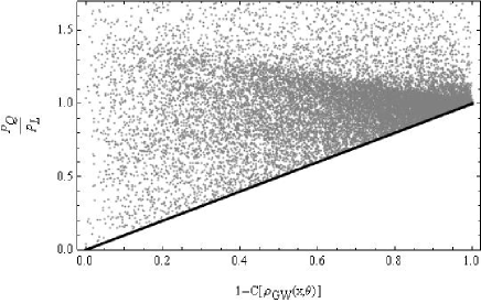
Figure 1: Plot of 20000 randomly generated sets of entangled $\rho_{GW}$ and unit vectors $(\mathbf{A},\mathbf{B})$ in the plane of $P_{Q}(\rho_{GW})/P_{L}(\rho_{GW})\sim 1-\mathcal{C}(\rho_{GW})$ in company with the line of $P_{Q}(\rho_{GW})/P_{L}(\rho_{GW})=1-\mathcal{C}(\rho_{GW})$.

II.3 Mixture of a Bell State and a Diagonal State

Another generalization of Werner state is the Bell State $|\psi^{+}\rangle$ mixed with a diagonal state

$$\rho_{BD}=\begin{bmatrix}\ x+\gamma/2&0&0&\gamma/2\\ \ 0&a&0&0\\ \ 0&0&b&0\\ \ \gamma/2&0&0&y+\gamma/2\end{bmatrix},$$ (32)

where the non-negative real parameters $x+y+a+b+\gamma=1$. It contains many special two-qubit states, such as maximally entangled mixed states $\rho_{MEMS}$ MEMS , frontier states of the bounds for concurrence RhoFr and so on. Its concurrence is $\mathcal{C}(\rho_{BD})=\max\{0,\gamma-2\sqrt{ab}\}$, which is independent on $x$ and $y$. Our construction of the EPR2 decomposition of $\rho_{BD}$ is divided into two steps: (i) We give the results of the spacial case of $x=y=0$; (ii) The local distribution of the general case can be derived immediately based on the results of the first step.

(i) When $x=y=0$, $\rho^{0}_{BD}=\gamma|\psi^{+}\rangle\langle\psi^{+}|+a|01\rangle\langle 01|+b|10\rangle\langle 10|$, and the quantum probability distribution is

$$P_{Q}(\rho^{0}_{BD})=\frac{1}{4}[1+(a-b)(A_{z}-B_{z})+(\gamma-a-b)A_{z}B_{z}+\gamma(A_{x}B_{x}-A_{y}B_{y})],\ \$$ (33)

where we choose $a\geq b$ without loss of generality. At the critical point of separability $\gamma=2\sqrt{ab}$,

$$P_{L}^{c}(\rho^{0}_{BD}) = \frac{1}{4}[F^{+}_{A}(A_{x})F^{+}_{B}(B_{x})+F^{-}_{A}(A_{x})F^{-}_{B}(B_{x})+F^{+}_{A}(A_{y})F^{-}_{B}(B_{y})+F^{-}_{A}(A_{y})F^{+}_{B}(B_{y})]$$ (34)

$$= P_{Q}(\rho^{0}_{BD})|_{\gamma=2\sqrt{ab}}$$

where the local response functions $F^{\pm}_{A}(x)=\frac{1}{2}(1+\sin\vartheta A_{z}\pm\cos\vartheta x)$ and $F^{\pm}_{B}(x)=\frac{1}{2}(1-\sin\vartheta B_{z}\pm\cos\vartheta x)$, with $\vartheta=\vartheta_{c}=\arcsin(\sqrt{a}-\sqrt{b})$. In the region $\gamma<2\sqrt{ab}$, we assume

$$P_{L}(\rho^{0}_{BD}) = gP_{L}^{c}(\rho^{0}_{BD})+(1-g)P_{L}^{0}(\rho^{0}_{BD}),$$ (35)

$$P_{L}^{0}(\rho^{0}_{BD}) = \lambda_{+}F^{+}(A_{z})F^{-}(B_{z})+\lambda_{-}F^{-}(A_{z})F^{+}(B_{z}),$$

where $\lambda_{\pm}=\frac{1}{2}(1\pm\Delta)$ and $P_{L}^{0}(\rho^{0}_{BD})$ take the same form as $P_{Q}(\rho^{0}_{BD})|_{\gamma=0}$. To hold the relation $P_{L}(\rho^{0}_{BD})=P_{Q}(\rho^{0}_{BD})$ when $\gamma<2\sqrt{ab}$, the parameters should be chosen as $g=2\gamma/(\gamma+2\sqrt{ab})$ and $\Delta=(\sqrt{a}+\sqrt{b}-g)(\sqrt{a}-\sqrt{b})/(1-g)$, both of which lie in $[0,1]$. When $\rho^{0}_{BD}$ is entangled with $\gamma>2\sqrt{ab}$, the probability distribution (33) can be decomposed as

$$P_{Q}(\rho^{0}_{BD})=[1-\mathcal{C}(\rho^{0}_{BD})]P_{L}(\rho^{0}_{BD})+\mathcal{C}(\rho^{0}_{BD})P_{NL}(\rho^{0}_{BD}),\ \$$ (36)

where $P_{L}(\rho^{0}_{BD})$ takes the definition in Eq. (34) with $\vartheta=\arcsin[(\sqrt{a}-\sqrt{b})/(\sqrt{a}+\sqrt{b})]$ and $P_{NL}(\rho^{0}_{BD})=\frac{1}{4}(1+\mathbf{A}\cdot\mathbf{B^{\prime}})$ corresponding to the probability distribution of the Bell state $|\psi^{+}\rangle$.

(ii) An arbitrary state (32) can always be written as $\rho_{BD}=x|00\rangle\langle 00|+y|11\rangle\langle 11|+p\rho^{\prime}$, where $p=\gamma+a+b$ and $\rho^{\prime}=\rho^{0}_{BD}|_{(\gamma,a,b)\rightarrow(\gamma/p,a/p,b/p)}$. Its concurrence is $\mathcal{C}(\rho_{BD})=p\mathcal{C}(\rho^{\prime})$. One can obtain immediately

$$P_{Q}(\rho_{BD})=pP_{Q}(\rho^{\prime})+xF^{+}(A_{z})F^{+}(B_{z})+yF^{-}(A_{z})F^{-}(B_{z}).\ \$$ (37)

In the approach given in step (i), $P_{Q}(\rho^{\prime})$ can be divided into the local $P_{L}(\rho^{\prime})$ and nonlocal $P_{NL}(\rho^{\prime})$ parts, with the wights $1-\mathcal{C}(\rho^{\prime})$ and $\mathcal{C}(\rho^{\prime})$ respectively. Choosing the construction $P_{L}(\rho_{BD})=[p(1-\mathcal{C}(\rho^{\prime}))P_{L}(\rho^{\prime})+xF^{+}(A_{z})F^{+}(B_{z})+yF^{-}(A_{z})F^{-}(B_{z})]/[p(1-\mathcal{C}(\rho^{\prime}))+x+y]$, one has

$$P_{Q}(\rho_{BD})=[1-\mathcal{C}(\rho_{BD})]P_{L}(\rho_{BD})+\mathcal{C}(\rho_{BD})P_{NL}(\rho^{\prime}),$$ (38)

in which the nonlocal probability distribution is the same as the one of $\rho^{\prime}$.

III conclusion and discussion

In conclusion, we investigate the EPR2 decomposition of the probability distribution arising from single-copy von Neumann measurements on arbitrary two-qubit states. In our constructive proof, the local content is shown to have a lower bound connected with the concurrence which measures the degree of entanglement, $p_{L}^{\max}\geq 1-\mathcal{C}(\rho)$. The local probability distribution for two families of mixed states are constructed independent of the scheme in the proof. Both of them lead to the local weight $p_{L}=1-\mathcal{C}(\rho)$.

In this paper, what we concern about are the mixed states of a two-qubit system. A natural extension of this issue is to study the EPR2 decomposition in a bipartite arbitrary-dimensional system. To our knowledge, only in Scarani’s paper Scarani2008 , a one-parameter family of two-qutrit states has been investigated in the EPR2 approach. For the state $|\Psi(\gamma)\rangle=(|00\rangle+|11\rangle+\gamma|22\rangle)/\sqrt{2+\gamma^{2}}$, Scarani chose the local distribution $P_{L}$ to be the product of Kronecker deltas $\delta_{\alpha,i(A)}$ and $\delta_{\beta,j(B)}$, where $i(A)$ and $j(B)$ are the most probable local outcomes when $\gamma>1$. His numerical results show the local content is nonzero when $\gamma>2$. However, an analytic lower bound of $p_{L}$ is absent. We would like to present our prospects to give an improved lower bound and generalize it to the mixed states case. (i) We start from the one-parameter state $|\Psi(\gamma)\rangle$ and construct a local distribution $P_{L}$ which is a function of the parameter $\gamma$. The Kronecker deltas can be represented as $\delta_{\alpha,i(A)}=\frac{1}{3}\{1+2\cos\frac{2\pi}{3}[\alpha-i(A)]\}$ and $\delta_{\beta,j(B)}=\frac{1}{3}\{1+2\cos\frac{2\pi}{3}[\beta-j(B)]\}$, in which the cosine functions play the roles of $\alpha\mathrm{sgn}(a_{z})$ and $\beta\mathrm{sgn}(b_{z})$ in the original construction of the qubit case given by EPR2 EPR2 . To obtain an improved lower bound of $p^{max}_{L}$, one can choose an appropriate function to substitute for the cosine function, like Scarani introducing the function $f(x)$ in Eq. (11) to take the place of the sign function. (ii) A subsequent work is to extend the results of the one-parameter state to the Schmidt-decomposed state $|\Phi(\gamma_{1},\gamma_{2})\rangle=(|00\rangle+\gamma_{1}|11\rangle+\gamma_{2}|22\rangle)/\sqrt{1+\gamma_{1}^{2}+\gamma_{2}^{2}}$. Obviously, the lower bound of $p^{max}_{L}$ for $|\Phi(\gamma_{1},\gamma_{2})\rangle$ should be a function of the parameters $\gamma_{1}$ and $\gamma_{2}$, and afterward, be a function of the entanglement invariants of the two-qutrit state Fei . (iii) Based on the results in the first two steps, one can attempt to decompose some typical mixed two-qutrit states in the EPR2 approach. In the light of the experience in Sec. II, an alternative construction of the local distribution $P_{L}$ has the form of a linear combination of the pure states case. And it is often effective to start from the critical point of separability.

References

• (1) A. Einstein, B. Podosky, and N. Rosen. Phys. Rev. 47 (1935) 777.
• (2) J. S. Bell. Physics 1 (1964) 195.
• (3) R. F. Werner. Phys. Rev. A 40 (1989) 4277.
• (4) N. Gisin. Phys. Lett. A 154 (1991) 201.
• (5) M. A. Nielsen and I. L. Chuang. Quantum Computation and Quantum Information. Cambridge University Press, Cambridge (2000) .
• (6) C. H. Bennett and S. J. Wiesner. Phys. Rev. Lett. 69 (1992) 2881.
• (7) A. K. Ekert. Phys. Rev. Lett. 67 (1991) 661.
• (8) A. Acín, N. Brunner, N. Gisin, S. Masser, S. Pironio, and V. Scarani. Phys. Rev. Lett. 98 (2007) 230501.
• (9) C. H. Bennett, D. P. DiVincenzo, J. A. Smolin, and W. K. Wootters. Phys. Rev. A 54 (1996).
• (10) S. Hill and W. K. Wootters. Phys. Rev. Lett. 78 (1997) 5022.
• (11) W. K. Wootters. Phys. Rev. Lett. 80 (1998) 2245.
• (12) C. H. Bennett, G. Brassard, S. Popescu, B. Schumacher, J. Smolin, and W. K. Wootters. Phys. Rev. Lett. 76 (1996) 722.
• (13) V. Vedral, M. B. Plenio, K. Jacobs, and P. L. Knight. Phys. Rev. A 56 (1997) 4452.
• (14) K. Życzkowski, P. Horodecki, A. Sanpera, and M. Lewenstein. Phys. Rev. A 58 (1998) 883.
• (15) G. Vidal and R. F. Werner. Phys. Rev. A 65 (2002) 032314.
• (16) A. Elitzur, S. Popescu, and D. Rohrlich. Phys. Lett. A 162 (1992) 25.
• (17) J. Barrett, A. Kent, and S. Pironio. Phys. Rev. Lett. 97 (2006) 170409.
• (18) V. Scarani. Phys. Rev. A 77 (2008) 042112.
• (19) D.-L. Deng and J.-L. Chen. Annals of Physics 373 (2009) 1616.
• (20) W. J. Munro, D. F. V. James, A. G. White, and P. G. Kwiat. Phys. Rev. A 64 (2001) 030302(R).
• (21) J. Barrett. Phys. Rev. A 65 (2002) 042302.
• (22) G. Tóth and A. Acín. Phys. Rev. A 74 (2006) 030306(R).
• (23) A. Acín, N. Gisin, and B. Toner. Grothendieck’s constant and local models for noisy entangled quantum states. Phys. Rev. A 73 (2006) 062105. doi:10.1103/PhysRevA.73.062105.
• (24) Z. Ma, F.-L. Zhang, D.-L. Deng, and J.-L. Chen. Phys. Lett. A 324 (2009) 408.
• (25) S. Albeverio and S. M. Fei. J. Opt. B: Quantum Semiclass Opt 3 (2001) 223.